A computational study of auditory models in music recognition tasks for normal-hearing and hearing-impaired listeners

R E S E A R C H

Open Access

A computational study of auditory

models in music recognition tasks for

normal-hearing and hearing-impaired listeners

Klaus Friedrichs

, Nadja Bauer

, Rainer Martin

and Claus Weihs

Abstract

The benefit of auditory models for solving three music recognition tasks—onset detection, pitch estimation, and instrument recognition—is analyzed. Appropriate features are introduced which enable the use of supervised classification. The auditory model-based approaches are tested in a comprehensive study and compared to state-of-the-art methods, which usually do not employ an auditory model. For this study, music data is selected according to an experimental design, which enables statements about performance differences with respect to specific music characteristics. The results confirm that the performance of music classification using the auditory model is comparable to the traditional methods. Furthermore, the auditory model is modified to exemplify the decrease of recognition rates in the presence of hearing deficits. The resulting system is a basis for estimating the intelligibility of music which in the future might be used for the automatic assessment of hearing instruments.

Keywords: Music recognition, Classification, Onset detection, Pitch estimation, Instrument recognition, Auditory model, Music intelligibility, Hearing impairment

1 Introduction

Hearing-impaired listeners like to enjoy music as well as normal-hearing listeners although this is impeded by a distorted perception of music signals. Recently, several listening experiments have been conducted to assess the impact of hearing loss on music perception for hearing-impaired listeners (e.g., [1–4]). For many applications like optimization of hearing instruments, it is desirable to measure this impact automatically using a simula-tion model. Therefore, we investigate the potential of emulating certain normal-hearing and hearing-impaired listeners by automatically assessing their ability to discriminate music attributes via an auditory model. Auditory models are computational models which mimic the human auditory process by transforming acoustic signals into neural activity of simulated auditory nerve fibers (channels). Since these models do not explain the whole listening comprehension of higher central auditory stages, a back end is needed relying on the output of the auditory periphery. Similar ideas have already been

*Correspondence: friedrichs@statistik.tu-dortmund.de

1_{Department of Statistics, TU Dortmund University, 44221 Dortmund, Germany} Full list of author information is available at the end of the article

proposed for measuring speech intelligibility in [5, 6] where this back end is an automatic speech recognition system, resulting in the word recognition rate as a natural metric. However, no such straightforward method exists to measure the corresponding “music intelligibility” in general. Unlike speech, music spectra are highly variable and have a much greater dynamic range [7]. For estimat-ing “music intelligibility,” its constituent elements (pitch, harmony, rhythm, and timbre) have to be assessed in an independent manner [8]. Therefore, we focus on three separate music recognition tasks, i.e., onset detection, pitch estimation, and instrument recognition. Contrary to state-of-the-art methods, here, we extract informa-tion from auditory output only. In fact, some recent proposals in the field of speech recognition and music data analysis use auditory models, thus exploiting the superiority of the human auditory system (e.g., [9–11]). However, in most of these proposals, the applied audi-tory model is not sufficiently detailed to provide adequate options for implementing realistic hearing deficits. In the last decades, auditory models have been developed which are more sophisticated and meanwhile can simu-late hearing deficits [12–15]. In [16, 17], it is shown that

simple parameter modifications in the auditory model are sufficient to realistically emulate auditory profiles of hearing-impaired listeners.

In this study, we restrict our investigation on chamber music which includes a predominant melody instrument and one or more accompanying instruments. For fur-ther simplification, we are only interested in the melody track which means that all accompanying instruments are regarded as interferences. This actually means that the three recognition tasks are described more precisely as predominant onset detection, predominant pitch estima-tion, and predominant instrument recognition.

The article is organized as follows. In Section 2, related work is discussed. The contribution of this paper is sum-marized in Section 3. In Section 4, the applied auditory model of Meddis [18] (Section 4.1) and our proposals for the three investigated music recognition tasks are described (Sections 4.2–4.4). At the end of that section, the applied classification methods—Random Forest (RF) and linear SVM—are briefly explained (Section 4.5). Section 5 provides details about the experimental design. Plackett-Burman (PB) designs are specified for selecting the data set, which enable assessments about perfor-mance differences w.r.t. the type of music. In Section 6, we present the experimental results. First, the proposed approaches are compared to state-of-the-art methods, and second, performance losses due to the emulation of hearing impairments are investigated. Finally, Section 7 summarizes and concludes the paper and gives some suggestions for future research.

2 Related work

Combining predominant onset detection and predomi-nant pitch estimation results in a task which is better known as melody detection. However, the performance of approaches in that research field are rather poor to date compared to human perception [19]. In particular, onset detection is still rather error-prone for polyphonic music [20]. Hence, in this study, all three musical attributes of interest are estimated separately, which means the true onsets (and offsets) are assumed to be known for pitch estimation and instrument recognition, excluding error propagation from onset detection.

2.1 Onset detection

The majority of onset detection algorithms consists of optional pre-processing stage, a reduction function (called onset detection function), which is derived at a lower sampling rate, and a peak-picking algorithm [21]. They all can be summarized into one algorithm with sev-eral parameters to optimize. In [22], we systematically solve this by using sequential model-based optimiza-tion. The onset detection algorithm can also be applied channel-wise to the output of the auditory model where

each channel corresponds to a different frequency band. Here, the additional challenge lies in the combination of different onset predictions of several channels. In [23], a filter bank is used for pre-processing, and for each band, onsets are estimated which together build a set of onset candidates. Afterwards, a loudness value is assigned to each candidate and a global threshold and a minimum dis-tance between two consecutive onsets are used to sort out candidates. A similar approach, but this time for combin-ing the estimates of different onset detection functions, is proposed in [24] where the individual estimation vec-tors are combined via summing and smoothing. Instead of combining the individual estimations at the end, in [25], we propose a quantile-based aggregation before peak-picking. However, the drawback of this approach is that the latency of the detection process varies for the dif-ferent channels, which is difficult to compensate before peak-picking. Onset detection of the predominant voice is a task which to our best knowledge has not been investigated, yet.

2.2 Pitch estimation

Most pitch estimation algorithms are either based on the autocorrelation function (ACF), or they work in the fre-quency domain by applying a spectral analysis of potential fundamental frequencies and their corresponding par-tials. For both approaches, one big challenge is to pick the correct peak which is particularly difficult for polyphonic music where the detection is disturbed by overlapping partials. In order to solve that issue, several improvements are implemented in the popular YIN algorithm [26] which in fact uses the difference function instead of the ACF. A further extension is the pYIN method which is introduced in [27]. It is a two-stage method which takes past estima-tions into account. First, for every frame, several funda-mental frequency candidates are predicted, and second, the most probable temporal path is estimated, according to a hidden Markov model. In [28], a maximum-likelihood approach is introduced in the frequency domain. Another alternative is a statistical classification approach which is proposed in [29].

are originally designed for monophonic pitch detection. However, pitch estimation can be extended to its pre-dominant variant by identifying the most pre-dominant pitch, which many peak-picking methods implicitly calculate.

Also for polyphonic pitch estimation, approaches exist. One approach is proposed in [10]. Instead of just picking the maximum peak of the SACF, the strength of each candidate (peak) is calculated as a weighted sum of the amplitudes of its harmonic partials. Another approach is introduced in [32], where the EM algorithm is used‘ to estimate the relative dominance of every possible harmonic structure.

2.3 Instrument recognition

The goal of instrument recognition is the automatic detec-tion of music instruments playing in a given music piece. Different music instruments have different compositions of partial tones, e.g., in the sound of a clarinet, mostly odd partials occur. This composition of partials is, how-ever, also dependent on other factors like the pitch, the room acoustic, and the performer [33]. For building a classifier, meaningful information of each observation has to be extracted, which is achieved by appropriate fea-tures. Timbral features based on the one-dimensional acoustic waveform are the most common features for instrument recognition. However, features based on an auditory model have also been introduced in [34]. Also, biomimetic spectro-temporal features, requiring a model of higher central auditory stages, have been successfully investigated for solo music recordings in [35]. Predomi-nant instrument recognition can be solved similarly to the monophonic variant, but is much harder due to the addi-tional “noise” from the accompanying instruments [36]. An alternative is starting with sound source separation in order to apply monophonic instrument recognition after-wards [37]. Naturally, this concept can only work if the sources are well separated, a task which itself is still a challenge.

3 Contribution of the paper

As there exist only very few approaches for music recog-nition tasks using a comprehensive auditory model, in this study, new methods are proposed. For onset detection, we adapt the ideas of [23, 24] to develop a method for combining onset estimations of different channels. The main drawback of the approach in [23] is that the selection procedure of onset candidates is based on a loudness esti-mation and a global threshold which makes it unsuitable for music with high dynamics. Instead, in [24] and also in our approach, relative thresholds are applied. However, the proposal in [24] can only combine synchronous onset estimations, i.e., the same sampling rate has to be used for the onset detection functions of all basic estimators. Our new approach can handle asynchronous estimations

which enables the use of different hop sizes. Furthermore, we propose parameter optimization to adapt the method to predominant onset detection. Sequential model-based optimization (MBO) is applied to find optimal parameter settings for three considered variants of onset detection: (1) monophonic, (2) polyphonic, and (3) predominant onset detection. For pitch estimation, inspired by [29], we propose a classification approach for peak-picking, where each channel nominates one candidate.

In [29], potential pitch periods derived from the origi-nal sigorigi-nal are used as features, whereas in our approach, features need to be derived using the auditory model. Our approach is applicable to temporal autocorrelations as well as to frequency domain approaches. Addition-ally, we test the SACF method, where we investigate two variants for peak-picking. For instrument recognition, we adapt common timbral features for instrument recogni-tion by extracting them channel-wise from the auditory output. This is contrary to [34], where the features are defined across all channels. The channel-wise approach preserves more information, can be more easily adapted to the hearing-impaired variants, and enables assessments of the contribution of specific channels to the recognition rates.

All approaches are extensively investigated using a comprehensive experimental design. The experimental setup is visualized in Fig. 1. The capability of audi-tory models to discriminate the three considered music attributes is shown via the normal-hearing auditory model which is compared to the state-of-the-art methods. For instrument recognition, the approach using the auditory model output even performs distinctly better than the approach using standard features. As a prospect of future research, performance losses based on hearing deficits are exemplified using three so-called hearing dummies as introduced in [17].

4 Music classification using auditory models

4.1 Auditory models

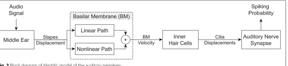
The auditory system of humans and other mammals con-sists of several stages located in the ear and the brain. While the higher stages located in the brainstem and cor-tex are difficult to model, the auditory periphery is much better investigated. This stage models the transformation from acoustical pressure waves to release events of the auditory nerve fibers. Out of the several models simu-lating the auditory periphery, we apply the popular and widely analyzed model of Meddis [18], for which simu-lated hearing profiles of real hearing impaired listeners exist [17].

Fig. 1Structure of the experiments for the music recognition tasks

transmits vibrations to the stapes in the middle ear and then further to the cochlea in the inner ear. Inside the cochlea, a traveling wave deflects the basilar membrane at specific locations dependent on the stimulating fre-quencies. On the basilar membrane, inner hair cells are activated by the velocity of the membrane and evoke spike emissions (neuronal activity) to the auditory nerve fibers. The auditory model of Meddis [18] is a cascade of several consecutive modules, which emulate the spike firing process of multiple auditory nerve fibers. A block diagram of this model can be seen in Fig. 2. Since auditory models use filter banks, the simulated nerve fibers are also called channels within the simulation. Each channel cor-responds to a specific point on the basilar membrane. In the standard setting of the Meddis model, 41 channels are examined. As in the human auditory system, each channel has an individual best frequency (center frequency) which defines the frequency that evokes maximum excitation. The best frequencies are equally spaced on a log scale with 100 Hz for the first and 6000 Hz for the 41st channel.

In the last plot of Fig. 3, an exemplary output of the model can be seen. The 41 channels are located on the vertical axis according to their best frequencies. The grayscale indicates the probability of spike emissions (white means high probability). The acoustic stimulus of this example is a harmonic tone which is shown in the first plot of the figure. The first module of the Meddis model corresponds to the middle ear where sound waves

are converted into stapes displacement. The resulting output of the sound example is shown in the second plot. The second module emulates the basilar membrane where stapes displacement is transformed into the velocity of the basilar membrane at different locations, implemented by a dual-resonance-non-linear (DRNL) filter bank, a bank of overlapping filters [38]. The DRNL filter bank consists of two asymmetric bandpass filters which are processed in parallel: one linear path and one nonlinear path. The output of the basilar membrane for our sound example can be seen in the third plot of the figure. Next, time-dependent basilar membrane velocities are transformed into time-dependent inner hair cell cilia displacements. Afterwards, these displacements are transformed by a calcium-controlled transmitter release function into spike probabilities p(t,k), the final output of the considered model, where t is the time, and k is the channel num-ber. For details about the model equations, the reader is refered to the appendix in [18].

For the auditory model with hearing loss, we con-sider three examples, called “hearing-dummies,” which are described in [16, 17]. These are modified versions of the Meddis auditory model. The goal of the hearing-dummies is to mimic the effect of real hearing impairments [39]. In the original proposal [17], channels with best frequen-cies between 250 Hz and 8 kHz are considered, whereas in the normal-hearing model described above, channel fre-quencies between 100 Hz and 6 kHz are used. Note that

Fig. 3Exemplary output of Meddis’ model of the auditory periphery: (1) original signal (200 Hz + 400 Hz), (2) middle ear output (stapes displacement), (3) basilar membrane (BM) output with respect to the channels’ best frequencies (BF), (4) auditory nerve (AN) output with respect to the BFs

this difference is just a matter of the user’s interesting frequency range and not influenced by any hearing dam-age. For a better comparison, the same best frequencies will be taken into account for all models. Since the range between 100 Hz and 6 kHz seems to be more suitable to music, we adjust the three hearing-dummies accordingly.

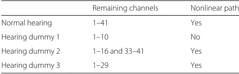
The first hearing dummy simulates a strong mid- and high-frequency hearing loss. In the original model, this is implemented by retaining the channel with the best fre-quency of 250 Hz only and by disabling the nonlinear path. In our modified version of that dummy, the first ten channels are retained—all of them having best frequencies lower than or equal to 250 Hz—and the nonlinear path is disabled for all of them. The second hearing dummy simulates a mid-frequency hearing loss indicating a clear dysfunction in a frequency region between 1 and 2 kHz. Therefore, we disable 16 channels (channels 17 to 32) for the modified version of the hearing dummy. The third hearing dummy is a steep high-frequency loss, which is implemented by disabling all channels with best frequen-cies above 1750 Hz corresponding to the last 12 channels in the model. The parameterization of the three hearing dummies is summarized in Table 1.

4.2 Onset detection

The task of onset detection is to identify all time points where a new tone begins. For predominant onset

detection, just the onsets of the melody track are of inter-est. First, we define the baseline algorithm which operates on the acoustic waveformx[t]. Second, we adapt this algo-rithm to the auditory model output in a channel-wise manner. Third, we describe the performed parameter tun-ing which we apply to optimize onset detection. Last, we introduce our approaches using the auditory model by aggregating the channel-wise estimations.

4.2.1 Baseline onset detection approach

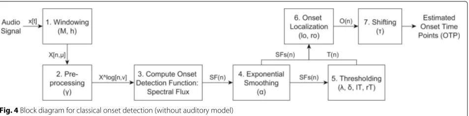
The baseline onset detection approach we use in our study consists of seven steps illustrated in Fig. 4. The corresponding parameters, used for the optimization, are shown in parentheses.

In the first step, the incoming signal is split into small frames with a frame size of M samples and a hop size hwhich is the distance in samples between the starting

Table 1Parameterization of the three considered hearing dummies and the normal hearing model

Remaining channels Nonlinear path

Normal hearing 1–41 Yes

Hearing dummy 1 1–10 No

Hearing dummy 2 1–16 and 33–41 Yes

Fig. 4Block diagram for classical onset detection (without auditory model)

points of subsequent frames. For each frame, the mag-nitude spectrum of the discrete Fourier transform (DFT) |X[n,μ]|is computed wherendenotes the frame index and μ the frequency bin index. Afterwards, two pre-processing steps are applied (step 2). First, a filter-bank F[μ,ν] filters the magnitude spectrum according to the note scale of western music [40]. The filtered spectrum is given by

Xfilt[n,ν]= M

μ=1

|X[n,μ]| ·F[μ,ν] , (1)

whereνis the bin index of this scale which consists ofB= 82 frequency bins (12 per octave), spaced in semitones for the frequency range from 27.5 Hz to 16 kHz. Second, the logarithmic magnitude of the spectrum is computed:

Xlog[n,ν]=log(γ·Xfilt[n,ν]+1), (2)

whereγ ∈] 0, 20] is a compression parameter to be opti-mized.

Afterwards, a feature is computed in each frame (step 3). Here, we use the spectral flux (SF(n)) feature, which is the best feature for onset detection w. r. t. the F mea-sure according to recent studies. In [41], this is shown on a music data set with 1065 onsets covering a variety of musi-cal styles and instrumentations, and in [40], this is verified on an even larger data set with 25,966 onsets. Spectral flux describes the degree of positive spectral changes between consecutive frames and is defined as:

SF(n)=

B

ν=1

H(Xlog[n,ν]−Xlog[n−1,ν])

withH(x)=(x+ |x|)/2.

(3)

Joining the feature values over all frames consecutively yields the SF vector.

Next, exponential smoothing (step 4) is applied, defined by

SFs(1)=SF(1)and

SFs(n)=α·SF(n)+(1−α)·SFs(n−1) for n=2,. . .,L,

(4)

whereLis the number of frames andα∈[ 0, 1].

A threshold function (step 5) distinguishes between rel-evant and nonrelrel-evant maxima. To enable reactions to dynamic changes in the signal, a moving threshold is applied, which consists of a constant partδand a local part weighted byλ[41]. The threshold function is defined as

T(n)=δ+λ·mean(SFs(n−lT),. . ., SFs(n+rT)),

for n=1,. . .,L, (5)

wherelT andrT are the number of frames to the left and

to the right, respectively, defining the subset of considered frames.

The localized tone onsets are selected by two conditions (step 6):

O(n)= ⎧ ⎨ ⎩

1, if SFs(n) >T(n)and SFs(n)= max(SFs(n−lO),. . ., SFs(n+rO)) 0, otherwise.

(6)

O = (O(1),. . .,O(L))T is the tone onset vector and lO

andrO are additional parameters, representing again the

number of frames to the left and right of the actual frame. Frames withO(n) = 1 are converted into time points by identifying their beginnings (in seconds). Finally, all estimated onset time points are shifted by a small time constantτ (step 7) to account for the latency of the detec-tion process. Compared to the physical onset, which is the target in our experiments, the perceptual onset is delayed, affected by the rise times of instrument sounds [42]. In the same manner, these rise times also affect the maximum value of spectral flux and other features.

Then, OTP = (OTP1,. . ., OTPCest) denotes the

resulting vector of these final estimates, whereCestis the number of estimated onsets. A found tone onset is cor-rectly identified if it is inside a tolerance interval around the true onset. We use±25 ms as the tolerance which is also used in other studies [40].

The performance of tone onset detection is measured by theF-measure taking into account the tolerance regions:

F= 2·mT+ 2·mT++mF++mF−

where m_T+ is the number of correctly detected onsets, m_F+is the number of false alarms, andm_F−is the number of missed onsets.F = 1 represents an optimal detection, whereasF =0 means that no onset is detected correctly. Apart from these extremes, theF-measure is difficult to interpret. Therefore, we exemplify the dependency of the number of missed onsets on the number of true onsets Ctrue=mT++mF−and theFvalue for the scenario where

no false alarm is produced:

mF+ =0 =⇒ mF−=

1− F 2−F

×Ctrue. (8)

In a listening experiment, we would assume a rela-tively low number of false alarms. Hence, we will use the scenariomF+ =0 for a comparison to human perception.

4.2.2 Parameter optimization

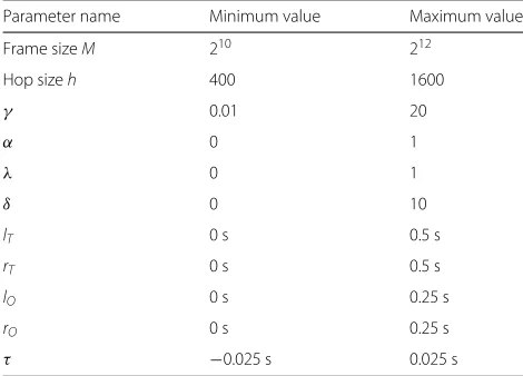
The baseline onset detection algorithm contains the 11 parameters summarized in Table 2. Parameter optimization is needed to find the best parameter setting w.r.,t. a training data set and to adapt the algorithm to predominant onset detection and to the auditory model output. Since evaluation of one parameter setting—also called point in the following—is time consuming (5 to 15 min on the used Linux-HPC cluster system [43]), we apply sequential model-based optimization (MBO). After an initial phase, i.e., an evaluation of some ran-domly chosen starting points, new points are proposed and evaluated iteratively w.r.t. a surrogate model fitted to all previous evaluations, and an appropriate infill cri-terion decides which point is the most promising. The most prominent infill criterion is expected improvement (EI) which looks for a compromise of surrogate model uncertainty in one point and its expected function value. For a more detailed description of MBO, see [44, 45].

Table 2Parameters and their ranges of interest for the classical onset detection approach

Parameter name Minimum value Maximum value

Frame sizeM 210 ₂12

Hop sizeh 400 1600

γ 0.01 20

α 0 1

λ 0 1

δ 0 10

lT 0 s 0.5 s

rT 0 s 0.5 s

lO 0 s 0.25 s

rO 0 s 0.25 s

τ −0.025 s 0.025 s

4.2.3 Onset detection using an auditory model

The baseline onset detection algorithm can also be per-formed on the output of each channel of the auditory modelp(t,k). Again, we use MBO to optimize the algo-rithm on the data, this time individually for each channel k, getting the estimation vectorOTPk. Now, the additional

challenge arises how to combine different onset predic-tions of several channels. We compare two approaches. First, as a simple variant, we just consider the channel which achieves the best F-value on the training data. Second, we introduce a variant which combines the final results of all channels. This approach is illustrated in Fig. 5. Again, the parameters we want to optimize are shown in parentheses.

Since particularly the performance of the highest channels are rather poor as we will see in Section 6, and furthermore, considering that fewer channels lead to a reduction of computation time, we allow the omission of the lowest and the highest channels by defining the minimum kmin and the maximum channel kmax. All estimated onset time points of the remaining channels are pooled into one set of onset candidates:

OTPcand = kmax

k=kmin

OTPk. (9)

Obviously, in this set, many estimated onsets occur several times, probably with small displacements, which have to be combined to a single estimation. Additionally, estimations which just occur in few channels might be wrong and should be deleted. Hence, we develop the following method to sort out candidates. For each estima-tion, we count the number of estimations in their temporal neighborhood, defined by an interval of±25 ms (corre-sponding to the tolerance of the F measure). In a next step, only estimations remain where this count is a local maximum above a global threshold. The threshold is defined by

β·(kmax−kmin+1), (10)

whereβ is a parameter to optimize. For each candidate time pointn, the interval within which it must fulfill the maximum condition is set to [n−tloc,. . .,n+tloc], where tlocis another parameter to optimize.

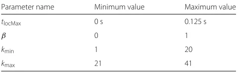
This results in four free parameters which we optimize in a second MBO run. The ranges of interest for these parameters are listed in Table 3. Since optimizing just four parameters is much faster than optimizing the eleven parameters of the conventional method, the overhead of computation time can be ignored.

Fig. 5Block diagram for the proposed approach for onset detection using an auditory model

target time points (not including the onset time points of the accompaniment).

4.3 Predominant pitch estimation

Here, we understand pitch estimation as a synonym for fundamental frequency (F0) estimation, where we allow a tolerance of a half semitone (50 cents). This is equivalent to a relative error of approximately 3% on the frequency scale (Hz). In the predominant variant, we are just inter-ested in the pitch of the melody instrument. As already mentioned above, we assume that the onsets and offsets of each melody tone are known. This information is used to separate the auditory output of each song temporally into individual melody tones (including the accompaniment at this time).

Our tested approaches using the auditory model can be divided into two groups—autocorrelation approach and spectral approach—which are described in the fol-lowing. Additionally, we use the YIN algorithm [26] and its extension pYIN [27], which do not employ an auditory model, for comparison reasons in our experi-ments. The mean error rate over all tones is applied to measure the performances of the approaches, i.e., it is assumed that all tones are equally important, regardless of their length.

4.3.1 Autocorrelation approach

One challenge of autocorrelation analysis of the auditory output is again the combination of several channels. In [30, 31], this is achieved by first computing the individual running autocorrelation function (ACF) of each channel and combining them by summation (averaging) across all channels (SACF). The SACF is defined by

Table 3Parameters and their ranges of interest for the aggregation approach (onset detection with auditory model)

Parameter name Minimum value Maximum value

tlocMax 0 s 0.125 s

β 0 1

kmin 1 20

kmax 21 41

s(t,l)= 1 K

K

k=1

h(t,l,k), (11)

where K is the number of considered channels and h(t,l,k) is the running ACF of each auditory channel k at time t and lag l. The peaks of the SACF are indica-tors for the pitch where the maximum peak is a promising indicator for the fundamental frequency. The model is successfully tested for several psychophysical phenomena like pitch detection with missing fundamental frequency [30, 31]. However, for complex musical tones, often the maximum peak of the SACF is not located at the fun-damental frequency, but instead at one of its multiples. Hence, we propose an improved peak picking version which takes the first peak of the SACF which is above an optimized threshold:

min[t∈tlM: SACF(t) > λ·max(SACF(t))] , (12)

wheretlMis the set of all local maxima of the SACF and λ∈[0, 1] has to be optimized on a training set.

4.3.2 Spectral approach

We propose a classification method partly based on fea-tures which we introduced in [46, 47] for detecting the frequencies of all partials. Here, the feature set is adapted for pitch estimation and some additional features are added. At first, the DFT magnitude spectrum |P[μ,k]| of each auditory channel k is computed where each maximum peak within an interval around the channel’s best frequency—limited by the best frequencies of the two neighboring channels—is considered as the channel’s pitch candidate:

μ∗[k]= arg max μ∈{BF[k−1],...,BF[k+1]}

|P[μ,k]|, k=1,. . .,K,

(13)

The classification target is to identify the channel with minimal distance between its best frequency and the fundamental frequency. The frequency candidate of this channel is returned as the estimated pitch. The follow-ing features are computed individually for each channel respectively and for each candidate:

• The frequency of the candidatec[k],

• The spectral amplitude of the candidate’s frequency

bin:ac[k]= |P[μ∗[k] ,k]|,

• The bandwidthb[k]of the candidate, defined by the

distance between the two closest frequency bins to the left and right of the candidate, where the spectral amplitude is below 10% of the candidate’s amplitude (see also Fig. 6):

b[k]=CF(μ∗_right[k])−CF(μ∗_left[k]). (14)

The band edges are defined by

μ∗right[k]=min

μ∈ μ∗[k] ,. . .,M 2

:

ac[k]

10 >|P[μ,k]|

,

(15)

Fig. 6Features for pitch estimation.aBandwidthb[k] of the candidate peak,bdistance to maximum leftdleft[k], andcdistance to

maximum rightdright[k]the candidate) across

whereμ∗_right[k]is set toM₂, if no suchμexists, and

μ∗

left[k]=max

μ∈ {1,. . .,μ∗[k]}:

ac[k]

10 >|P[μ,k]|

,

(16)

whereμ∗_left[k]is set to 0, if no suchμexists,

• The distances of the candidate’s frequency to the

maxima to the left and right, respectively, restricted by the candidate’s band edges (two features:dleft[k] anddright[k], see also Fig. 6):

dleft[k]=c[k]−CF(mleft[k]),where m_left[k]= arg max

μ∈{1...μ∗ left[k]}

(P[μ,k])and (17)

dright[k]=CF(mright[k])−c[k] ,where mright[k]= arg max

μ∈μ∗ right[k]...

M 2

(P[μ,k]). (18)

• The spectral amplitude of these two maxima (2

features):|P[mleft[k] ]|and|P[mright[k] ]|.

• Average and maximum spike probabilities of the

channel:pmean[k]andpmax[k],

• Average and maximum spectral magnitude of the

first nine partials (pl=1,. . ., 9) across all channels:

P_plmean[k]= 1 K

K

n=1

P[fb(pl·c[k]),n] , (19)

wherefb(i)is the frequency bin which comprises

frequencyiand

P_plmax[k])= max

n∈{1,...,K}(P[fb(pl·c[k]),n] ,), (20)

Studies have shown that humans can resolve the first 7 to 11 partials [48, 49]. Hence, the first nine partials might be beneficial for pitch estimation.

• In the same manner, average and maximum spectral

magnitude of the first undertone (half frequency of the candidate) across all channels:Pmean₁

2

[k]and

Pmax1 2

[k].

Altogether, this results in 29 features for each channel, i.e., 29 × 41 = 1189 features for the auditory model.

As a third method for pitch estimation, this classifica-tion approach is also applied in the same way to the ACF. Here, the same 29 features are extracted, but this time based on the ACF instead of the DFT.

4.4 Predominant instrument recognition

one could assume the same predominant instrument during one song, we do not use the information about previous tones, since we want to use instrument recog-nition as an indicator for correctly perceived timbre. We think this is best characterized by tone-wise classi-fication without using additional knowledge. Hence, also here, the auditory output of each song is separated into temporal segments defined by the individual tones of the predominant instrument, and for each segment— corresponding to one melody tone—features are extracted separately.

We use 21 features, listed in Table 4, which we already considered in previous studies [50]. These features are common for instrument recognition based directly on the time domain waveform and are linked to tim-bre in the literature [51]. For our approach using an auditory model, they are computed on each of the 41 channels, thus, we obtain 41 × 21 = 861 fea-tures for each tone. The first 20 feafea-tures are computed by means of theMIRtoolbox[52]. The last feature is the Shannon-Entropy:

H(X[μ])= −

M

μ=1

pr(|X[μ]|)log₂pr(|X[μ]|), (21)

where X[μ] is the DFT of a signal frame (respectively the DFT of a channel output in the auditory model vari-ant) and pr(|X[μ]|) = M|X[μ]|

ν=1|X[ν]|

is the share of the

μth frequency bin with respect to the cumulated spectral magnitudes of all bins.H(X[μ]) measures the degree of spectral dispersion of an acoustic signal and is taken as a measure for tone complexity.

4.5 Classification methods

Supervised classification is required for our approaches in pitch estimation and instrument recognition. Formally, a classifier is a mapf : →, where is the input space containing characteristics of the entities to classify and

Table 4Features for instrument recognition [50]

Feature no. Feature name

1 Root-mean-square energy

2 Low energy

3 Mean spectral flux (see Eq. 3)

4 Standard deviation of spectral flux

5 Spectral rolloff

6 Spectral brightness

7 Irregularity

8–20 Mel-frequency cepstral coefficients (mfcc):

First 13 coefficients

21 Entropy

is the set of categories or classes. Here, is a (reduced) set of features andis a set of labels of musical instruments or channels (pitch candidates).

In our experiment, we apply two important classes of methods, namely linear large margin methods (repre-sented by the linear support vector machine, SVM) and ensembles of decision trees (Random Forests, RF).

4.5.1 Decision trees and Random Forests

Decision trees are one of the most intuitive models used in classification. The model is represented as a set of hierarchical “decision rules,” organized usually in a binary tree structure. When a new observation needs to be classified, it is propagated down the tree tak-ing either the left or right branch in each decision node of the tree, depending on the decision rule of the current node and the corresponding feature value. Once a terminal node has been reached, a class label is assigned. For a more detailed description of decision trees, see [53].

Sometimes, a single classification rule is not powerful enough to sufficiently predict classes of new data. Then, one idea is to combine several rules to improve pre-diction. This leads to so-called ensemble methods. One example is Random Forests (RF), a combination of many decision trees (see, e.g., [54]). The construction of the dif-ferent classification trees has random components—i.e., for each tree, only a random subset of observations, and for each decision node, only a random subset of features is considered—leading to the term Random Forests.

4.5.2 Support vector machines

Support vector machines (SVMs) [55] are among the state-of-the-art machine learning methods for linear and non-linear classification. They are often among the strongest available predictors, and they come with exten-sive theoretical guarantees. To simplify our experimental design, we consider only linear SVMs.

The linear SVM separates two classes by a hyperplane maximizing a so-called safety margin between the classes. As we cannot exclude the existence of outliers, so-called slack variables are applied, one per training point, measur-ing the amount of margin violation. Overall, maximization of the margin is traded against minimization of margin violations.

4.5.3 Feature selection

Feature selection filters the important features in order to reduce computation time for feature extraction as well as for the classification process itself. Another advantage of feature selection is a better interpretability of a classi-fication model based on lesser features. Knowing which features are important might also help to design improved feature sets. Lastly, feature selection can even improve classification results since classifiers have problems with meaningless or redundant features.

Two basic approaches exist for feature selection: for-ward selection and backfor-ward selection [56]. Forfor-ward selection is a greedy search approach which starts with an empty set of features. In each iteration, the feature which yields the most improvement w.r.t. the error rate is added to the set until no feature yields an improvement higher than a specified threshold. Backward selection works the other way round. It starts with all features, and in each iteration, the feature is removed which yields the least improvement. Here, the stopping threshold is usually a small negative value allowing also small increases of the error rate in order to simplify the model.

Both approaches have a complexity of O(n2) which results in too much computation time when dealing with n ≈ 1000 features as we consider for pitch estima-tion and instrument recogniestima-tion. Hence, we propose to group the features into feature groups and to handle each group as one single feature for forward and backward selection, respectively. There are two natural grouping mechanisms since the features can be categorized by two dimensions: the channel index and the feature name. The first approach is to combine the related features across all channels into one group, and the second approach is to combine all features generated in the same channel into one group. The first approach results in 29 feature groups for pitch estimation and 21 groups for instrument recog-nition. For both tasks, the second approach results inK feature groups. An additional benefit of channel-based grouping is the potential of sorting out entire channels which also reduces computation time for the simulated auditory process. In our experiments, we set the mini-mum improvement for forwards selection to 0.01 and for backward selection to−0.001.

5 Design of experiments

5.1 Data

Our data base consists of 100 chamber music pieces recorded in MIDI which include a specific melody instru-ment and one or more accompanying instruinstru-ments, either piano or strings. The ISP toolbox in Matlab with the “Fluid (R3) General MIDI SoundFont” is applied for synthesizing MIDI files in a sample-based way [57]. For simplifica-tion reasons, only standard playing styles are considered, e.g., bowed for cello. Naturally, real music recordings

would be preferable, but the chosen concept provides a labeled data base with onset times, pitches, and the instru-ments being played which is sufficiently large to apply our experimental design.

In most studies of music data, experiments are per-formed on a rather arbitrary data base of music samples where it is difficult to determine how well it represents a whole entity of music. Instead, we construct a more structured data base using an experimental design based on eight musical factors which might have an influence on music intelligibility. This enables identification of the most problematic music w.r.t. classification performance. We apply Plackett-Burman (PB) designs which require just two levels for each factor [58]. After all experiments (music samples) are evaluated, a linear regression model is fitted to predict the target variables w.r.t. the factor levels. For onset detection, the target variable is theF measure; for instrument recognition, it is the classification error rate; and for pitch estimation, it is the mean error rate using a tolerance of a half semitone. If no factor has a sig-nificant influence on the target variable, we can assume that the approach works equally well for all considered music pieces. The goodness of fit of the regression model is measured by the so-called R-squared (R2∈[0, 1]) which indicates the proportion of variance that is explained by the factors.R2= 1 means that the results are completely explained by the considered factors, whereas R2 = 0 means that the factor values do not influence the results, i.e., the results are independent of the type of music. Since R2_{also depends on the number of factors, adjustedR}2_are used to compensate this effect [59]:

R2_a=1− nexp−1 nexp−pfac−1(

1−R2), (22)

wherenexp is the number of experiments andpfac is the number of factors [60].

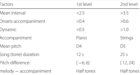
the two levels is ensured. The factors of the first group are as follows:

• Mean interval size: This is the mean interval step

between two consecutive tones of the melody, measured in semitones. We define two factor levels: <2.5and>3.5.

• Onsets in accompaniment: This factor defines the

common individual onsets produced by the accompanying instrument(s) which do not occur in the track of the melody instrument w.r.t. to all onsets. We apply two factor levels:<0.4and>0.6.

• Dynamics: We define the dynamics of a song by the

mean absolute loudness difference of consecutive melody tones, measured in MIDI velocity numbers. We consider two factor levels:<0.5and>1.0.

• Accompanying instrument: We consider two

instruments as factor levels: piano and strings.

The four factors of the second group can take values which are, within limits, freely adjustable:

• Melody instrument: We consider three instruments

of different instrument groups as factor levels: cello, trumpet, and clarinet. Here, no natural aggregation into two factor levels exist. Hence, it is not

considered within the PB designs, and instead, the designs are repeated three times, one repetition for each instrument.

• Mean pitch of the melody: We restrict the minimum

and maximum allowed pitches for the melody to the pitch range of the three considered instruments which is from E3 (165 Hz) to A6 (1047 Hz). For the experimental design, we define two levels. The first level transposes the song extract (including the accompaniment) such that the average pitch of the melody is D4 (294 Hz), and the second level transposes the song extract such that the average pitch of the melody is D5 (587 Hz). Afterwards, we apply the following mechanism to prevent unnatural pitches w.r.t. the instruments. If the pitch of one tone violates the allowed pitch range, the pitch of all tones within the considered song extract is shifted until all pitches are valid.

• Tone duration: We define the factor tone duration by

the duration of the song extracts in order to maintain the rhythmic structure. If this factor is modified, all tone lengths of the song extract are adjusted in the same way. We consider two factor levels: 12 and 25 s which, for our data, results in tone lengths between 0.1 and 0.5 s for the first level and between 0.2 and 1.0 s for the second level.

• Mean pitch of accompaniment: This factor is the

difference of the average pitch of the accompaniment compared to the average pitch of the melody. For

changing this factor, we only permit transpositions of the accompaniment tracks by full octaves (12 semitones). The two considered levels are defined by the intervals [−6,6] and [−24,−12] measured in semitones. If the pitches of melody and

accompaniment are similar, we expect higher error rates for the considered classification tasks. The case where the accompaniment is significantly higher than the melody is neglected since this is rather unusual at least for western music.

The factors and their specified levels are summarized in Table 5. We apply PB designs with 12 experiments and pfac=7 factors (as noted above the melody instrument is not considered within the PB design) to generate appro-priate song extracts. Each experiment defines one specific combination of factor levels. First, for each experiment, all possible song extracts with a length of 30 melody tones are identified from our data base of 100 MIDI songs w.r.t. the specification of the first factor group. Second, for each experiment, one of these song extracts is chosen and the factors of the second group are adjusted as defined by the design. Finally, each song extract is replicated three times, changing the melody instrument each time. Overall, this results in 3× 12×30 = 1080 melody tones for each PB design. We apply three independent designs and choose different song excerpts in order to enable cross-validation. Hence, we getnexp = 3 × 12 = 36 experiments alto-gether. To ensure that the accompaniment is not louder than the melody, we use a melody to accompaniment ratio of 5 dB.

5.2 Structure of the comparison experiments

At first, the approaches described in the previous section are compared using the original auditory model without a simulated hearing loss. The structure of the whole process is illustrated in Fig. 1.

For all experiments, threefold cross-validation is applied which means the excerpts of two designs are used for training of the classification models—or in the optimization stage in case of onset detection—and the

Table 5Plackett-Burman designs: factor levels

Factors 1st level 2nd level

Mean interval <2.5 >3.5

Onsets accompaniment <0.4 >0.6

Dynamic <0.5 >1.0

Accompaniment Piano Strings

Mean pitch D4 D5

Song (tone) duration 12 s 25 s

Pitch difference: [−6, 6] [ 12, 24]

remaining excerpts of the third design are used for test-ing. Additionally, the approaches are also compared on monophonic data using the same excerpts but without any accompanying instruments. Without any distortion by the accompaniment, misclassification rates should be marginal.

Since the predominant variant of onset detection is a novel issue, a comparison to existing approaches is difficult. Searching for all onsets, as well as the mono-phonic case, are the standard problems of onset detection. Hence, apart from the monophonic and the predominant variant, we also investigate the approaches w. r. t. usual polyphonic onset detection (all onsets). All nine cases— three approaches (two with and one without an auditory model) combined with the three variants—are individ-ually optimized using MBO with 200 iterations, which means 200 different parameter settings are tested on the training data.

For pitch estimation and instrument recognition, all classification approaches are tested in two variants: RF and linear SVM (Section 4.5). For instrument recogni-tion, features are extracted from the auditory model or the original signal which results in four considered vari-ants altogether. For pitch estimation, eleven approaches are compared: four classification approaches with auditory features—RF or SVM combined with DFT or ACF features—(Section 4.3.1), two peak-picking vari-ants for the SACF approach (Section 4.3.2) and five variants of the YIN (respectively pYIN) algorithm as the state-of-the-art approaches without an auditory model.

For the YIN algorithm, standard settings are used, except for the lower and the upper limits of the search range which are set to 155 and 1109 Hz, respectively. These values corresponds to the pitch range of the melody in the considered song extracts. In contrast to the other tested approaches, the YIN and the pYIN algorithms estimate the fundamental frequency for short frames and not for complete tones. Hence, an aggregation mecha-nism is needed to aggregate the fundamental frequency estimations of several frames into one estimation for the complete tone. For the YIN algorithm, three aggregation approaches are tested. The first method selects the esti-mation of the frame which has the smallest “aperiodic power” component which might be an indicator for the estimation uncertainty [26]. The second method returns the median estimation. This method is also tested for the pYIN algorithms which, however, often wrongly estimates a higher partial. This effect might be rectified by lower quantiles, and hence, we also test the 10% quantile for YIN and pYIN.

For pitch and instrument recognition, the feature selec-tion approaches, described in Secselec-tion 4.5.3, are used to investigate the importance of channels (best frequencies) and features. Finally, all experiments conducted for the

auditory model without hearing loss are repeated for the three hearing dummies described in Section 4.1. This means also the optimization stage of onset detection and the training stages of pitch and instrument recognition are conducted separately for each hearing model.

5.3 Software

For classification, the R packagemlr[61] is applied using the packagerandomForest [62] for RFs and the package kernlab[63] for SVMs. MBO is performed by using the R packagemlrMBO[64]. Finally, the huge number of experi-ments performed is managed by the R packagesBatchJobs andBatchExperiments[65].

6 Results

First, we present the main results regarding the normal hearing auditory model in comparison to the reference approaches (Section 6.1). Second, we consider the perfor-mance loss of models with hearing deficits exemplified by the three hearing-dummies (Section 6.2).

6.1 Comparison of proposed approaches

We will look at the results of onset detection, pitch estimation, and instrument recognition, consecutively.

6.1.1 Onset detection

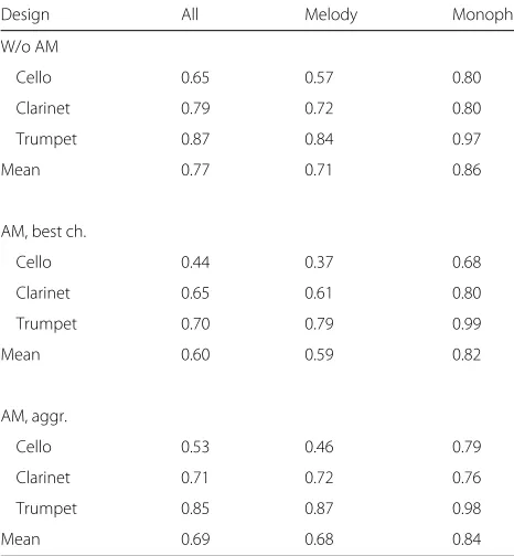
Table 6 shows the results of onset detection for the three considered approaches: (1) common onset detec-tion on the original signal (without any auditory model),

Table 6Results (mean F measure) for onset detection with and without an auditory model (AM)

Design All Melody Monoph.

W/o AM

Cello 0.65 0.57 0.80

Clarinet 0.79 0.72 0.80

Trumpet 0.87 0.84 0.97

Mean 0.77 0.71 0.86

AM, best ch.

Cello 0.44 0.37 0.68

Clarinet 0.65 0.61 0.80

Trumpet 0.70 0.79 0.99

Mean 0.60 0.59 0.82

AM, aggr.

Cello 0.53 0.46 0.79

Clarinet 0.71 0.72 0.76

Trumpet 0.85 0.87 0.98

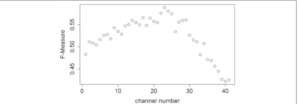
(2) onset detection using the auditory model output by choosing the output of the best single channel, and (3) onset detection where the estimated onset time points of several channels are combined. For all approaches, the rel-evant parameters are separately optimized for three tasks: monophonic onset detection (songs without accompani-ment), predominant onset detection where we are just interested in the melody onsets, and onset detection where we are interested in all onsets.

All approaches perform worse than expected, even the reference approach without the auditory model, which is the state-of-the-art method for monophonic data. Solving onset detection by using only one of the auditory chan-nels performs very differently from channel to channel as can be seen in Fig. 7. For the predominant task, channels with a medium best frequency are better than low and high channels. The best performance is achieved by using the output of channel 23 resulting in an averageF value of 0.59. However, the approach which aggregates the final estimations of all channels improves this result. Interest-ingly, in the optimum, all channels are considered, also the highest ones which individually perform very poorly as we have seen above. The averageFvalue of 0.68 in the pre-dominant variant is still slightly worse than the common onset detection approach based on the original signal. However, the aggregation is based on a relatively simple classification approach, which uses just the number of estimations in the neighborhood as a single feature.

In all variants, the performance for trumpet—which has a clear attack—is by far the best, whereas in most variants, the performance for cello is the worst. In the predom-inant variant, the detection of cello tones is even more difficult when it is disturbed by string accompaniment. Note that a comparison of different approaches for a spe-cific instrument should be done with care, since only the overall performance is optimized. This means, e.g., a small

loss of performance for trumpet might be beneficial if this leads to a bigger gain for cello or clarinet. As expected, the results for the polyphonic variants are distinctly worse than for the monophonic variant. Furthermore, finding all onsets seems to be simpler than finding just the melody onsets, at least for the considered melody to accompani-ment ratio of 5 dB.

In Table 7, the evaluation of the experimental design for the channel-aggregating method, averaged over the three instruments, can be seen. In the monophonic vari-ant, the adjustedR2(R2_a) is negative, which indicates that the performance is independent of the type of music. This is also supported by the p values, since none of them shows a significant impact. Obviously, this was expected for some factors which correspond to the accompaniment so that they should only have an impact in the polyphonic case. However, before conducting the experiments, we expected that greater values of themean intervalshould simplify onset detection.

For the other two variants of onset detection, the good-ness of fit is relatively high R2_a>0.5—note that we describe music pieces by just eight dimensions which explains the relatively high amount of noise in all eval-uation models of the experimental design. Nevertheless, we can identify some important influence factors w.r.t. the performance of the proposed algorithm. In the pre-dominant variant, the performance is better if the number of onsets solely produced by the accompaniment is low. Obviously, this was expected since false alarms caused by tones of the accompaniment are decreased in that case. However, a higher mean pitch and shorter tones also seem to be beneficial. In the polyphonic variant, piano accom-paniment is better than string accomaccom-paniment. This effect is explained by the bad performance of onset detection for string instruments in general as we have already seen for cello. Furthermore, also in this scenario, a smaller number

Table 7Evaluation over all instruments and all Plackett-Burman designs for the proposed aggregation approach (factors as in Table 5)

a b c

Fit R2_=0.13,R2

a= −0.09 R2=0.65,R2a=0.56 R2=0.61,R2a=0.51

Factors Estimates pvalue Estimates pvalue Estimates pvalue

(Intercept) 0.8448 _<2e−16 _{0.6815 <2e}−16 _{0.6945 <2e}−16

Mean interval −0.0015 0.90 −0.0041 0.76 0.0308 0.17

Onsets accompaniment −0.0021 0.87 −0.0636 4e−05 _{−0.0448 0.05}

Dynamic −0.0146 0.25 −0.0186 0.17 −0.0019 0.93

Accompaniment 0.0177 0.16 −0.0109 0.41 −0.1313 2e−06

Mean pitch 0.0029 0.81 0.0510 6e−04 _{0.0198 0.37}

Tone duration −0.0087 0.49 −0.0348 0.01 −0.0026 0.91

Pitch: mel. - acc. 0.0051 0.68 −0.0224 0.10 −0.0213 0.34

The averageFvalue is the target variable—a: monophonic onset detection, b: predominant onset detection, and c: polyphonic onset detection (italics= significant at 10% level)

of individual onsets produced by the accompaniment is beneficial, probably because mutual onsets of melody and accompaniment are easier to identify.

Comparison to human perception Although there is a wide range of publications dealing with the human per-ception of rhythm (see [66] for an overview), none of them analyzes the human ability to recognize onsets in musi-cal pieces. Reason for this might be the fact that onset detection is a rather trivial task for normal-hearing listen-ers at least for chamber music. This is particularly the case for monophonic music where only the detection of very short tones and the separation of two identical consecu-tive tones of bowed instruments seem to be challenging. According to Krumhansl, the critical duration between two tones for event separation is 100 ms [66], a threshold which is exceeded for all pairs of tones in this study.

An informal listening test with our monophonic music data indicates that even all onsets of identical consecu-tive tones can be identified by a trained normal-hearing listener. However, to study a worst-case scenario, let us assume (s)he does not recognize these onsets in case of the cello. That means, 94 out of the 3240 onsets are missed which corresponds to a misclassification rate of 2.9% and an F value of 0.99. Contrary, even the state-of-the-art method without the auditory model achieves a mean F value of only 0.86 which, according to (8), means that 24.6% of all onsets are missed if we assume that the algo-rithm does not produce any false alarm. In conclusion, in the field of automatic onset detection, big improvements are necessary in order to emulate human perception.

6.1.2 Pitch estimation

Table 8 lists the average error rates of pitch detection using the methods described in Section 4.3 for the three instru-ments. Additionally, the results for the monophonic data are listed. Out of the approaches with auditory model,

our approach using spectral features of the auditory out-put and a linear SVM for classification performs best with a mean error rate of 7% in the polyphonic and 2% in the monophonic case. The YIN algorithm with median aggregation performs even better with a mean error rate of only 3% for polyphonic music, whereas the “aperiodic power” variant performs extremely poor. The pYIN algo-rithm performs worse than the YIN algoalgo-rithm. Reason for this is that it more often confuses the frequency of a higher partial with the fundamental frequency. Paradox-ically, this effect occurs even more often in the mono-phonic variant. Contrary, all other approaches perform as expected clearly better in the monophonic variant than in the polyphonic one. Applying the 10% quantile instead of the median decreases the confusion of the higher par-tials and improves the performance which, nevertheless,

Table 8Mean error rates of pitch detection methods (italics indicates the best results for the mean performance)

Polyphonic/predominant Mono.

Method Cello Clar. Trump. Mean Mean

SACF max. 0.55 0.52 0.54 0.54 0.20

SACF thresh. 0.24 0.12 0.17 0.18 0.05

DFT + RF 0.14 0.02 0.08 0.08 0.02

DFT + SVM 0.11 0.01 0.08 0.07 0.02

ACF + RF 0.24 0.08 0.30 0.20 0.05

ACF + SVM 0.21 0.05 0.24 0.17 0.04

YIN + aperiodic power 0.36 0.15 0.32 0.28 0.05

YIN + median 0.04 0.01 0.04 0.03 0.00

YIN + 10% quantile 0.11 0.04 0.09 0.08 0.03

pYIN + median 0.04 0.17 0.07 0.09 0.12

is distinctly worse than the YIN algorithm with median aggregation.

Interestingly, clarinet tones are the main challenge for pYIN, whereas for all other approaches, the error rates for clarinet are the lowest and cello tones seem to be the most difficult ones. In general, the pitch of clarinet tones is eas-ier to estimate because these tones have a relatively low intensity of the even partials which might prevent octave errors. For trumpet and cello tones, often the frequency of the second partial is confused with the fundamental frequency. Again, pitches of cello tones which are accom-panied by string instruments are especially difficult to estimate.

For the best method with auditory model—the classifi-cation approach using spectral features and either linear SVM or RF—group-based feature selection is performed (as introduced in Section 4.5.3. The corresponding results are listed in Table 9. Especially, feature-based grouping shows good results. For both classification methods, the forward variant finishes with just two feature groups— instead of 29 without feature selection—where the perfor-mance reduction is only small. Interestingly, the two clas-sifiers choose different features. For RF,c[k] anddright[k] are picked, whereas for SVM, pmean[k] andPmean1 [k] are chosen. In the backward variant, the SVM just needs the following nine feature groups to achieve the same error rate as with all features: c[k], pmean[k], pmax[k], b[k],dleft[k],dright[k],P₄mean[k],Pmean₈ [k], andPmean₉ [k]. All other features might be meaningless or redundant.

Also some channels can be omitted: For classification with SVM, 23 channels instead of all 41 are sufficient to get the best error rate of 0.07. The ignored channels are located in all regions, which means no priority to lower or higher channels can be observed, and the crucial informa-tion is redundant in neighboring (overlapping) channels.

Table 10a shows the evaluation of the experimental design. The goodness of fitR2_a=0.12is rather low but some weakly significant influence factors can be identi-fied. For example, a bigger distance between the average pitch of melody and accompaniment seems to be advan-tageous. This was expected, since a bigger distance leads to a lesser number of overlapping partials. Additionally, there is a small significant influence regarding the kind of accompaniment: piano accompaniment seems to be

beneficial. Again, this is expected as it is difficult to distinguish cello tones from tones of other string instru-ments.

Comparison to human perception There exist several studies which investigate the ability of human pitch per-ception (see [66, 67] for an overview). In most of these studies, the ability to recognize relative changes of consec-utive tones is quantified. Frequency differences of about 0.5% can be recognized by a normal-hearing listener [68]. However, quantifying these differences is a much harder challenge. Discriminating thresholds for this task are in the magnitude of a semitone for listeners without musi-cal training which corresponds to a frequency difference of approximately 6% [69]. The ability to recognize such relative changes is called relative pitch which is the nat-ural way most people perceive pitches. However, relative pitch remains poorly understood, and the standard view of the auditory system corresponds to absolute pitch since common pitch models make absolute, rather than rela-tive, features of a sound’s spectrum explicit [67]. In fact, also humans can perceive absolute pitch. It is assumed that this requires acquisition early in life. Also abso-lute pitch possessors make errors—most times octave and semitone errors—whose rate varies strongly between individuals [70].

In conclusion, comparing the results of our study to human data constitutes a big challenge. We can assume that a normal-hearing listener might be able to perceive relative pitches almost perfectly w.r.t. the tolerance of

1

2 semitone at least in the monophonic case. This esti-mation approximately corresponds to the result of the classification method with DFT features which yields a mean error rate of 2% in our study. The human ability for the perception of polyphonic music has not yet been adequately researched to make a comparison. Hence, in future studies, extensive listening tests are necessary.

6.1.3 Instrument recognition

The error rates for instrument recognition are listed in Table 11. Here, the auditory model-based features per-form distinctly better than the standard features. In both cases, the linear SVM performs slightly better than the RF. Distinguishing trumpet from the rest seems to be slightly

Table 9Feature selection for pitch classification with auditory model and DFT: number of selected features and error rates

Method No selection Channel groups Feature groups

Forward Backward Forward Backward

RF: number of features 41× 29 = 1189 4 ×29 = 116 35×29 = 1015 41×2 = 82 41× 28= 1148

RF: error rate 0.08 0.10 0.07 0.09 0.08

SVM: number of features 41×29 = 1189 5 ×29 = 145 23×29 = 667 41×2 = 82 41× 9 = 369

Table 10Evaluation over all instruments and all Plackett-Burman Designs (factors as in Table 5)

a b

Fit R2_=0.30,R2

a=0.12 R2=0.37,R2a=0.21

Coefficients Estim. pvalue Estim. pvalue

(Intercept) 0.0660 2e−08 _{0.0111 9e}−04

Interval −0.0074 0.40 0.0049 0.11

Onsets acc. 0.0056 0.53 0.0037 0.23

Dynamic −0.0142 0.11 −0.0019 0.54

Acc. 0.0148 0.10 0.0056 0.07

Mean pitch −0.0068 0.44 0.0062 0.05

Tone dur. ₋0.0025 0.78 0.0025 0.42

Mel.₋acc. ₋0.0185 0.04 ₋0.0056 0.07

The error rate is the target variable— a: pitch estimation and SVM (auditory model + DFT), b: instrument recognition and SVM (auditory model features)—(italics= significant at 10% level)

more difficult than identifying cello or clarinet. In the monophonic variant, the results are nearly perfect for all variants. Since the auditory model-based features are only beneficial in the polyphonic case, we conclude that these features enhance the ability to separate individual voices or instruments.

Table 12 shows the result of feature selection for instru-ment recognition. Here, both backward variants even slightly improve the no-selection result for RF. Using only the features of 12 channels leads to the best result which is equally good as the SVM with all features. The selected channels are 8, 12, 19, 21, 22, 24, 26, 27, 28, 32, 33, and 41. Comparing the best frequencies of these channels and the pitch range of the melody explains why the low chan-nels are unimportant. The fundamental frequency of the considered melody tones is between 165 and 1047 Hz, corresponding to the channels 6 to 24 which have best frequencies between 167 and 1053 Hz. Also, some of the higher channels are important which supply information about overtones and possibly the fine structure. How-ever, the deselection of several channels also illustrates the redundancy of neighboring channels.

According to the results of forward selection, two chan-nels are sufficient to get error rates of about 3%. Chanchan-nels 26 and 41 are chosen for RF and channels 29 and 41

for SVM. The gain of higher channels for instrument recognition is further illustrated in Fig. 8. Applying the features of one of the first channels leads to an error rate of almost 40%, whereas the features of the 41st channel generate a model with an error rate below 5%. This is also interesting for our examination of auditory models with hearing loss since usually particularly the higher channels are degraded the most. Also, in the backward variant of channel-based grouping, the lowest channels are omitted. In the feature-based forward variant, the same three fea-ture groups are selected for SVM and RF, respectively: mean spectral flux,root-mean-square energy,andspectral rolloff. In the backward variant using the SVM, these three features are also chosen and five additional ones: irregu-larityand the first, the third, the fourth, and the seventh MFCC coefficients.

Table 10b shows the evaluation of the experimental design for predominant instrument recognition. Here, the goodness of fit is moderateR2_a=0.21and three weakly significant influence factors can be identified. The most significant influence has the mean pitch, i.e., lower tones can be distinguished better. Also, string accompaniment affects the error rates more than piano accompaniment. Again, the reason might be the difficulty to distinguish cello from other string instruments. Additionally, a bigger distance between the pitches of melody and accompani-ment also seems to be beneficial.

Comparison to human perception Most studies about timbre in the field of music psychology try to quantify dis-similar ratings and analyze their correlations to physical features, whereas the common task in the field of music information retrieval is instrument recognition. Although both tasks are very similar, there exists one important difference which causes diverging results of the two dis-ciplines. Dissimilar ratings are subjective measures which rely on judgements of humans, whereas instrument recog-nition is a well-defined task [51]. Nevertheless, also, some studies have conducted experiments about the human ability to distinguish music instruments (see [71] for a tabular overview). The most comprehensive experiment is reported in [72], a listening experiment with music experts. The subjects had to distinguish isolated notes of

Table 11Mean error rates of instrument recognition methods (italics indicates the best result for the overall performance)

Polyphonic Monophonic

Method Cello vs. all Clarinet vs. all Trumpet vs. all Overall Overall

AM features, RF 0.012 0.017 0.029 0.019 0.002

AM features, SVM 0.007 0.007 0.014 0.011 0.001

Standard features, RF 0.044 0.034 0.052 0.063 0.000