The Thirty-Third AAAI Conference on Artificial Intelligence (AAAI-19)
Practical Algorithms for Multi-Stage
Voting Rules with Parallel Universes Tiebreaking
Jun Wang, Sujoy Sikdar, Tyler Shepherd
Zhibing Zhao, Chunheng Jiang, Lirong Xia
Rensselaer Polytechnic Institute 110 8th Street, Troy, NY, USA
{wangj38, sikdas, shepht2, zhaoz6, jiangc4}@rpi.edu, [email protected]
Abstract
STV and ranked pairs (RP) are two well-studied voting rules for group decision-making. They proceed in multiple rounds, and are affected by how ties are broken in each round. How-ever, the literature is surprisingly vague about how ties should be broken. We propose the first algorithms for computing the set of alternatives that are winners undersome tiebreak-ing mechanism under STV and RP, which is also known as parallel-universes tiebreaking (PUT). Unfortunately, PUT-winnersare NP-complete to compute under STV and RP, and standard search algorithms from AI do not apply. We propose multiple DFS-based algorithms along with pruning strate-gies, heuristics, sampling and machine learning to prioritize search direction to significantly improve the performance. We also propose novel ILP formulations for PUT-winners under STV and RP, respectively. Experiments on synthetic and real-world data show that our algorithms are overall faster than ILP.
1
Introduction
TheSingle Transferable Vote (STV)rule1is among the most popular voting rules used in real-world elections. According to Wikipedia, STV is being used to elect senators in Aus-tralia, city councils in San Francisco (CA, USA) and Cam-bridge (MA, USA), and more (Wikipedia 2018). In each round of STV, the lowest preferred alternative is eliminated, in the end leaving only one alternative, the winner, remain-ing.
This raises the question: when two or more alternatives are tied for last place, how should we break ties to elim-inate an alternative? The literature provides no clear an-swer. For example, see (O’Neill 2011) for a list of different STV tiebreaking variants. While the STV winner is unique and easy to compute for a fixed tiebreaking mechanism, it is NP-complete to compute all winners underall tiebreak-ing mechanisms. This way of defintiebreak-ing winners is called parallel-universes tiebreaking (PUT) (Conitzer, Rognlie, and Xia 2009), and we will therefore call themPUT-winnersin this paper.
Copyright c2019, Association for the Advancement of Artificial Intelligence (www.aaai.org). All rights reserved.
1
STV is also known asinstant runoff voting, alternative vote, orranked choice voting.
Ties do actually occur in real-world votes under STV. On Preflib (Mattei and Walsh 2013) data, 9.2% of profiles have more than one PUT-winner under STV. There are two main motivations for computing all PUT-winners. First, it is vital in a democracy that the outcome not be decided by an arbi-trary or random tiebreaking rule, which will violate the neu-tralityof the system (Brill and Fischer 2012). Second, even for the case of a unique PUT-winner, it is important to prove that the winner is unique despite ambiguity in tiebreaking. In an election, we would prefer the results to be transparent about who all the winners could have been.
A similar problem occurs in the Ranked Pairs (RP) rule, which satisfies many desirable axiomatic properties in so-cial choice (Schulze 2011). The RP procedure considers ev-ery pair of alternatives and builds a ranking by selecting the pairs with largest victory margins. This continues until ev-ery pair is evaluated, the winner being the candidate which is ranked above all others by this procedure (Tideman 1987). Like in STV, ties can occur, and the order in which pairs are evaluated can result in different winners. Unfortunately, like STV, it is NP-complete to compute all PUT-winners under RP (Brill and Fischer 2012).
More generally, the tiebreaking problem exists for a larger class of voting rules calledmulti-stage voting rules. These rules eliminate alternatives in multiple rounds, and the dif-ference is in the elimination methods. For example, in each round, Baldwin’s rule eliminates the alternative with the smallest Borda score, and Coombs eliminates the alterna-tive with highest veto score. Like STV and RP, comput-ing all PUT winners is NP-complete for these multi-stage rules (Mattei, Narodytska, and Walsh 2014).
To the best of our knowledge, no algorithm beyond brute-force search is known for computing PUT-winners under STV, RP, and other multi-stage voting rules. Given its im-portance as discussed above, the question we address in this paper is:
How can we design efficient, practical algorithms for computing PUT-winners under multi-stage voting rules?
Our Contributions. Our main contributions are the first practical algorithms to compute the PUT-winners for multi-stage voting rules: a depth-first-search (DFS) framework and integer linear programming (ILP) formulations.
rep-resent intermediate rounds in the multi-stage rule, each leaf node is labeled with a single winner, and each root-to-leaf path represents a way to break ties. The goal is to output the union set of winners on the leaves. See Figure 1 and Figure 2 for examples. To improve the efficiency of the algorithms, we propose the following techniques:
Pruning, which maintains a set ofknown winnersduring the search procedure and can then prune a branch if expanding a state can never lead to any new PUT-winner.
Machine-Learning-Based Prioritization, which aims at building a large known winner set as soon as possible by prioritizing nodes that minimize the number of steps to dis-cover a new PUT-winner.
Sampling, which build a large set of known winners before the search to make it easier to trigger the pruning conditions. Our main conceptual contribution is a new measure called
early discovery, wherein we time how long it takes to com-pute a given proportion of all PUT-winners on average. This is particularly important for low stakes and anytime applica-tions, where we want to discover as many PUT-winners as possible at any point during execution.
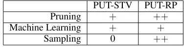
We will use STV and RP in this paper as illustrations for our framework. Experiments on synthetic and real-world data show the efficiency and effectiveness of our algorithms in solving the PUT problem for STV and RP, hereby de-noted PUT-STV and PUT-RP respectively. The effects of additional techniques compared to the standard DFS frame-work are summarized in Table 1, where the symbol++ de-notes very useful,+denotes mildly useful, and 0 denotes not useful.
PUT-STV PUT-RP
Pruning + ++
Machine Learning + +
Sampling 0 ++
Table 1: Summary of Technique Effectiveness.
It turns out that the standard DFS algorithm is already ef-ficient for STV, while various new techniques significantly improve running time and early discovery for RP.
In addition, we design an ILP for STV, and an ILP for RP based on the characterization by Zavist and Tideman (1989). For both PUT-STV and PUT-RP, in the large ma-jority of cases our DFS-based algorithms are orders of mag-nitude faster than solving the ILP formulations, but there are a few cases where ILP for PUT-RP is significantly faster. This means that both types of algorithm have value and may work better for different datasets.
Related Work and Discussions.There is a large literature on the computational complexity of winner determination under commonly-studied voting rules. In particular, com-puting winners of the Kemeny rule has attracted much at-tention from researchers in AI and theory (Conitzer, Daven-port, and Kalagnanam 2006; Kenyon-Mathieu and Schudy
2007). However, STV and ranked pairs have both been over-looked in the literature, despite their popularity. We are not aware of previous work on practical algorithms for PUT-STV or PUT-RP. A recent work on computing winners of commonly-studied voting rules proved that computing STV is P-complete, but only with a fixed-order tiebreaking mech-anism (Csar et al. 2017). Our paper focuses on finding all PUT-winners under all tiebreaking mechanisms. See (Free-man, Brill, and Conitzer 2015) for more discussions on tiebreaking mechanisms in social choice.
Standard procedures to AI search problems unfortunately do not apply here. In a standard AI search problem, the goal is to find a path from the root to the goal state in the search space. However, for PUT problems, due to the un-known number of PUT-winners, we do not have a clear pre-determined goal state. Other voting rules, such as Coombs and Baldwin, have similarly been found to be NP-complete to compute PUT winners (Mattei, Narodytska, and Walsh 2014). The techniques we apply in this paper for STV and RP can be extended to these other rules, with slight modifi-cation based on details of the rules.
2
Preliminaries
LetA ={a1,· · ·, am}denote a set ofmalternativesand letL(A)denote the set of all possible linear orders overA. Aprofileofnvoters is a collection P = (Vi)i≤n of votes where for each i ≤ n,Vi ∈ L(A). A voting rule takes as input a profile and outputs a non-empty set of winning alter-natives.
Single Transferable Vote (STV)proceeds inm−1rounds over alternativesAas follows. In each round, (1) an alterna-tive with the lowest plurality score is eliminated, and (2) the votes over the remaining alternatives are determined. The last-remaining alternative is the winner.
Figure 1: An example of the STV procedure.
Example 1. Figure 1 shows an example of how the STV procedure can lead to different winners depending on the tiebreaking rule. In round 1, alternativesBandC are tied for last place. For any tiebreaking rule in whichCis elim-inated, this leads toBbeing the winner. Alternatively, ifB were to be eliminated, thenAis the winner.
Ranked Pairs (RP). For a given profileP = (Vi)i≤n, we
define theweighted majority graph(WMG) ofP, denoted by wmg(P), to be the weighted digraph(A, E)where the nodes are the alternatives, and for every pair of alternatives
|{Vi:aVi b}| − |{Vi:bVi a}|. We define the
nonnega-tive WMGas wmg≥0(P) = (A,{(a, b)∈E:w(a,b)≥0}).
We partition the edges of wmg≥0(P)into tiersT1, ..., TKof edges, each with distinct edge weight values, and indexed according to decreasing value. Every edge in a tierTi has the same weight, and for any pairi, j ≤ n, ifi < j, then ∀e1∈Ti, e2∈Tj, we1> we2.
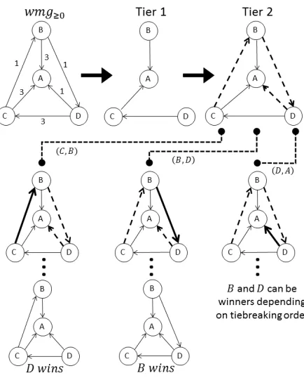
Figure 2: An example of the RP procedure.
Ranked pairs proceeds inKrounds: Start with an empty graphGwhose vertices areA. In each roundi ≤K, con-sider adding edgese ∈ Ti toGone by one according to a tiebreaking mechanism, as long as it does not introduce a cycle. Finally, output the top-ranked alternative inGas the winner.
Example 2. Figure 2 shows the ranked pairs procedure ap-plied to the WMG resulting from a profile overm= 4 alter-natives (a profile with such a WMG always exists) (McGar-vey 1953). We focus on the addition of edges in tier2, where
{(C, B),(B, D),(D, A)} are to be added. Note that D is the winner if(C, B)is added first , whileB is the winner if (B, D)is added first.
3
General Framework
We provide a general framework using a depth first search approach to solve multi-stage voting rules in Algorithm 1. Our algorithms for solving PUT-STV and PUT-RP are ex-amples of applying this common framework.
We evaluate our algorithms on two criteria:
(1) Total Running Timefor completing the search.
Algorithm 1General DFS-based framework. 1: Input:A profileP.
2: Output:All PUT-winnersW.
3: Initialize a stackF with the initial state;W =∅. 4: SamplePUT-winners randomly.
5: whileF is not emptydo
6: Pop a stateSfromF to explore.
7: ifShas a single remaining alternativethen 8: add it toW.
9: ifSalready visited or state can beprunedthen 10: skip state.
11: Expand current state to generate childrenC, addC
toF in order ofpriority.
12: returnW.
(2) Early Discovery.For any PUT-winner algorithm and any number0≤α≤1, theα-discovery value is the average running time for the algorithm to computeαfraction of PUT-winners.
The early discovery property is motivated by the need for any-time algorithms which, if terminated at any time, can output the known PUT-winners as an approximation to all PUT-winners. Such time constraint is realistic in low-stakes, everyday voting systems such as Pnyx (Brandt and Geist 2015), and it is desirable that an algorithm outputs as many PUT-winners as early as possible. This is why we fo-cus on DFS-based algorithms, as opposed to, for example, BFS, since the former reaches leaf nodes faster. We note that100%-discovery value can be much smaller than the to-tal running time of the algorithm, because the algorithm may continue exploring remaining nodes after100%discovery to verify that no new PUT-winner exists.
We propose several techniques to improve the running time and guide the search into promising branches contain-ing more alternatives that could be PUT-winners.
Pruning.The main idea is straightforward: if all candidate PUT-winners of the current state are already known to be PUT-winners, then there is no need to continue exploring this branch since no new PUT-winners can be found. Heuristic Functions. To achieve early discovery through Algorithm 1, we prioritize nodes whose state contains more candidate PUT-winners that have not been discovered. As a heuristic guided approach, we deviselocal priority func-tions which take as input the set of candidate PUT-winners (denoted by A) and the set of known PUT-winners (previ-ously discovered by the search, denoted byW) and output a priority order on the branches to explore in Line 11 of Al-gorithm 1. It is called local (as opposed to global) priority because overall the algorithm is still DFS, and the local pri-ority is used to decide which child of the current node will be expanded first.
•LP = |A−W|: Local priority; orders the exploration of children by the value of|A−W|, the number of potentially unknown PUT-winners.
proba-bility of a branch to have new PUT-winners, and prioritizing the exploration of branches with a higher estimated proba-bility of having new PUT-winners.
• LPML = P
a∈A−Wπ(a): Local priority with machine learning modelπ.
Hereπ(a)is the machine learning model probability ofa
to be a PUT-winner. The setup details can be found in Sec-tion 5. It is important to note we do not use the machine learning model to directly predict PUT-winners. Instead, we use it to guide DFS search to discover a new PUT-winner as soon as possible.
Sampling.Sampling in line 4 of Algorithm 1 can be seen as a preprocessing step: before running the search, we repeat-edly randomly sample a fixed tie-breaking orderπand run the voting procedure using π. If we can add PUT-winners earlier into the known winners set, the algorithm will earlier reach the pruning conditions during the search, eliminating branches.
PUT-STV as an Example.The framework in Algorithm 1 can be applied to PUT-STV with the following specifica-tions. We set the initial state inF to be the set of all alter-nativesA. We modify Step 11 of Algorithm 1 as: for every remaining lowest plurality score alternativec ∈S, in order ofpriorityadd (S\c) toF. For pruning specific to PUT-STV, we can skip the stateSwheneverS⊆W. We implement the heuristic functions LP and LPML to prioritize the order of exploring children, where the set of candidate PUT-winners
A is simply the remaining candidates of stateS. And we finally add sampling to our algorithms. The results are in Section 5.
4
Algorithms for PUT-RP
In this section we show how to adopt Algorithm 1 to com-pute PUT-RP. In the search tree, each node has a state
(G, E), whereEis the set of edges that have not been con-sidered yet andGis a graph whose edges are pairs that have been “locked in” by the RP procedure according to some tiebreaking mechanism. The root node is(G= (A,∅), E0), whereE0is the set of edges in wmg≥0(P).
At a high level, we have two ways to apply Algorithm 1. The first one is callednaive DFSbecause it is a straightfor-ward application of Algorithm 1, generating children at state
(G, E)by adding each edge in the highest weight edge tier ofEtoGthat does not cause a cycle. We also include our pruning conditions as detailed in this section.
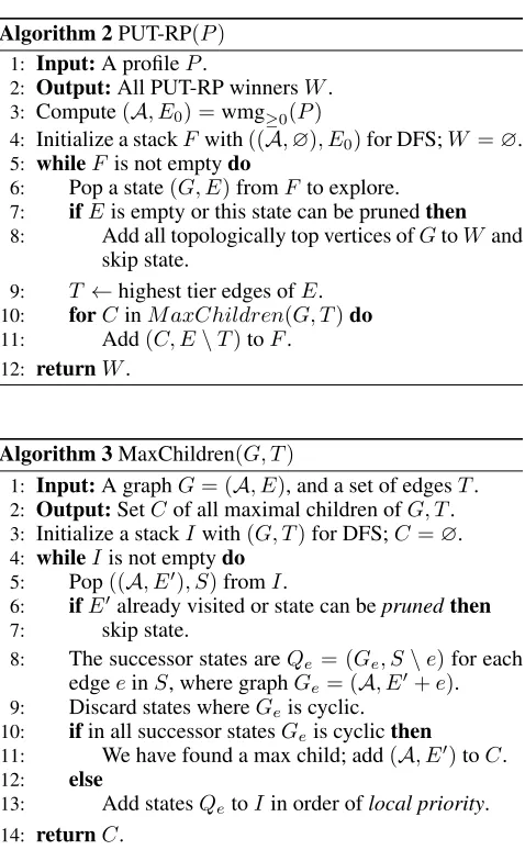
The second method is, in short, a layered algorithm in which we process edges tier by tier. It is described as the
P U T-RP() procedure in Algorithm 2. Exploring a node
(G, E) at depth t involves finding all maximal ways of adding edges fromTttoGwithout causing a cycle, which is done by theM axChildren()procedure shown in Algo-rithm 3.M axChildren()takes a graphGand a set of edges
Tas input, and follows a DFS-like addition of edges one at a time. Within the algorithm, each node(H, S)at depthd cor-responds to the addition ofdedges fromT toH according to some tiebreaking mechanism.S ⊆T is the set of edges not considered yet.
Definition 1. Given a directed acyclic graphG= (A, E),
and a set of edgesT, a graphC= (A, E∪T0)whereT0⊆
T is amaximal child of(G, T)if and only if∀e ∈ T\T0, addingeto the edges ofCcreates a cyclic graph.
Algorithm 2PUT-RP(P)
1: Input:A profileP.
2: Output:All PUT-RP winnersW. 3: Compute(A, E0) =wmg≥0(P)
4: Initialize a stackFwith((A,∅), E0)for DFS;W =∅. 5: whileF is not emptydo
6: Pop a state(G, E)fromFto explore. 7: ifEis empty or this state can be prunedthen 8: Add all topologically top vertices ofGtoWand
skip state.
9: T ←highest tier edges ofE. 10: forCinM axChildren(G, T)do 11: Add(C, E\T)toF.
12: returnW.
Algorithm 3MaxChildren(G, T)
1: Input:A graphG= (A, E), and a set of edgesT. 2: Output:SetCof all maximal children ofG, T. 3: Initialize a stackIwith(G, T)for DFS;C=∅. 4: whileIis not emptydo
5: Pop((A, E0), S)fromI.
6: ifE0already visited or state can beprunedthen 7: skip state.
8: The successor states areQe= (Ge, S\e)for each edgeeinS, where graphGe= (A, E0+e). 9: Discard states whereGeis cyclic.
10: ifin all successor statesGeis cyclicthen
11: We have found a max child; add(A, E0)toC. 12: else
13: Add statesQetoIin order oflocal priority. 14: returnC.
Therefore, the second algorithm will be called maximal children based (MC) algorithms. We have the following techniques for PUT-RP.
Pruning.For a graphGand a tier of edgesT, we imple-ment the following conditions to check if we can terminate exploration of a branch of DFS early: (i) If every alterna-tive that is not a known winner has one or more incoming edges or (ii) If all but one vertices inGhave indegree>0, the remaining alternative is a PUT-winner. For example, in Figure 2, we can prune the right-most branch after having explored the two branches to its left.
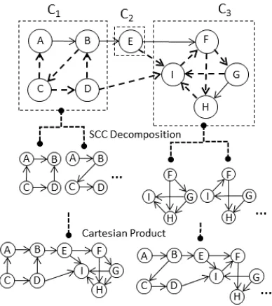
SCC Decomposition. We further improve Algorithm 3 by computing strongly connected components (SCCs). For a di-graph, an SCC is a maximal subgraph of the digraph where for each ordered pairu,vof vertices, there is a path fromu
tov. Every edge in an SCC is part of some cycle. The edges not in an SCC, therefore not part of any cycle, are called the bridge edges (Kleinberg and Tardos 2005, p. 98-99).
Figure 3: Example of SCC Decomposition.
children will be simpler if we can split it into multiple SCCs. We find the maximal children of each SCC, then combine them in the Cartesian product with the maximal children of every other SCC. Finally, we add the bridge edges.
Figure 3 shows an example of SCC Decomposition in which edges inGare solid and edges inT are dashed. Note this is only an example, and does not show all maximal chil-dren. In the unfortunate case when there is only one SCC we cannot apply SCC decomposition. The proof of Theorem 1 is provided in Appendices.
Theorem 1. For any directed graphH,Cis a maximal child ofH2if and only ifC contains exactly (i) all bridge edges
ofHand (ii) the union of the maximal children of all SCCs inH.
5
Experiment Results
5.1
Datasets
We use both synthetic datasets and real-world preference profiles from Preflib to test our algorithms’ performance. The synthetic datasets were generated based on impartial culture withnindependent and identically distributed rank-ings uniformly at random overmalternatives for each pro-file. From the randomly generated profiles, we only test on
hardcases where the algorithm encounters a tie that cannot be solved through simple pruning. All the following exper-iments are completed on a PC with Intel i5-7400 CPU and 8GB of RAM running Python 3.5.
Synthetic Data. For PUT-STV, we generate 10,000
m = n = 30 synthetic hard profiles. For PUT-RP, we
2
Here, we extend the definition of maximal child of directed graphH= (A, E)as the maximal child of the tuple(G, E)where G= (A,∅).
generate 14,875m=n= 10synthetic hard profiles. We let
m =nin our synthetic data because these are the hardest cases, which can be verified in Figure 4.
Figure 4: Running time of DFS for PUT-STV for different number of votersn, for profiles withm= 20candidates.
Preflib Data.We use all available datasets on Preflib suit-able for our experiments on both rules. Specifically, we use 315 profiles from Strict Order-Complete Lists (SOC), and 275 profiles from Strict Order-Incomplete Lists (SOI). They represent several real world settings including political tions, movies and sports competitions. For political elec-tions, the number of candidates is often not more than 30. For example, 76.1% of 136 SOI election profiles on Preflib has no more than 10 candidates, and 98.5% have no more than 30 candidates.
5.2
Results for PUT-STV
We test four variants of Algorithm 1 for PUT-STV: (i)DFS: Algorithm 1 with pruning but without local priority , (ii) LPML: Algorithm 1 with pruning and local priority based on machine learning, (iii)LPML+20msamples:its variants with20m= 600samples, and (iv)LPML+m sam-ples:m = 30samples. Results are summarized in Table 2 and Figure 5. The main conclusions are that DFS performs the best in total running time, local priority based on ma-chine learning (LPML) is useful for early discovery, and sampling is not useful. This makes sense because expand-ing nodes for STV is computationally easy, so the opera-tional cost of computing and maintaining a priority queue in LPML offsets the benefit of early discovery. All compar-isons are statistically significant with p-value=0.02 or less computed using one sided paired sample Student’s t-test.
Local Priority with Machine Learning Improves Early Discovery.As shown in Figure 5, form=n= 30, LPML has25.01%reduction in 50%-discovery compared to DFS. Results are similar for other datasets with differentm. The early discovery figure is computed by averaging the time to compute a given percentagepof PUT-winners. For example, for a profile with 2 PUT-winners which are discovered at timet1 andt2, we set the 10%-50% discovery time as t1
without sampling with sampling
DFS LPML LPML+600samples LPML+30samples Avg. running time (s) 0.4474 0.5017 0.6893 0.5252 Avg. 100%-discovery time (s) 0.1820 0.1686 0.3563 0.1826
Table 2: Experiment results of different algorithms for PUT-STV.
The π function used in the local priority function was trained by a neural network model using three hidden lay-ers with size of4096×1024×1024neurons and logistic function as activation, where the output hasmcomponents, each of which indicates whether the corresponding alterna-tive is a PUT-winner. The input features are the positional matrix, WMG, and plurality, Borda, k-approval, Copeland and maximin scores of the alternatives. We trained the mod-els on 50,000m=n= 30hard profiles using tenfold cross validation, with the objective of minimizing theL1-distance between the prediction vector and the target true winner vec-tor. Our mean squared error was 0.0833.
Figure 5: PUT-STV early discovery.m= 30.
Pruning Has Small Improvement. We see only a small improvement in the running time when evaluating pruning: on average, pruning brings only 0.33% reduction in running time for m = n = 10profiles, 2.26% form = n = 20
profiles, and 4.51% form=n= 30profiles.
Sampling Does Not Help.We test different number of sam-ples as shown in Figure 5 but none of them brings improve-ment. This is because each sample is essentially just a run of DFS up to leaf node, which is no different from our algo-rithm. Moreover, pruning has only small improvement since its condition is not often triggered, so knowing PUT-winners actually does no good to both early discovery and running time.
DFS Is Practical on Real-World Data.Our experimental results on Preflib data show that on 315 complete-order real world profiles, the maximum observed running time is only
0.06seconds and the average is 0.335 ms.
5.3
PUT-RP
We evaluate three algorithms together with their sampling variants for RP: (i) nDFS(LP):naive DFS (Algorithm 1) with pruning and local priority based on # of candidate PUT-winners, (ii) MC(LP):maximal children based algo-rithm with SCC decomposition (Algoalgo-rithm 2) and the same local priority as the previous one, and (iii) MC(LPML): its variant with a different local priority based on machine learning predictions. Experimental results are summarized in Table 3 and Figure 6. In short, the conclusion is that MC(LP) with sampling is the fastest algorithm for PUT-RP, and both the sampling variants of nDFS(LP) and MC(LP) perform well in early discovery. All comparisons are statis-tically significant with p-value≤0.01 unless otherwise men-tioned.
Pruning Is Vital.Pruning plays a prominent part in the re-duction of running time. Our contrasting experiment fur-ther justifies this argument: DFS without any pruning can only finish running on 531 profiles of our dataset before it gets stuck, taking 125.31 seconds in both running time and 100%-discovery time on average, while DFS with pruning takes only 2.23 seconds and 2.18 seconds respectively with a surprising 50 times speedup.
Local Priority Improves Early Discovery.In order to eval-uate its efficacy, we test the naive DFS without local pri-ority, and the average time for 100%-discovery is 0.9976 seconds, which is about 3 times of that for nDFS(LP)’s 0.2778 seconds. Note that naive DFS without local prior-ity is not shown in Figure 6. Local priorprior-ity with machine learning (LPML) does not help as much as LP. For LPML, we learn a neural network model using tenfold cross vali-dation on 10,000 hard profiles and test on 1,000 hard pro-files. The input features are the positional matrix, in- and out-degrees and plurality and Borda scores of all alternatives in the WMG.
Sampling Is Efficient. We test different algorithms with 200 samples and observe a large reduction in running time. The fastest combination is MC(LP) with sampling (in Ta-ble 3) with only 2.87s in running time and 0.08s in 100%-discovery time on average. Sampling has the least improve-ment with p-value 0.02 when applied to nDFS.
without sampling with sampling
nDFS(LP) MC(LPML) MC(LP) nDFS(LP) MC(LPML) MC(LP) Avg. running time (s) 7.6571 7.9858 7.7081 7.5291 3.0395 2.8692 Avg. 100%-discovery time (s) 0.2778 6.7876 6.4058 0.0531 0.2273 0.0823
Table 3: Experiment results for PUT-RP.
Figure 6: PUT-RP early discovery.
In both experiments, we omit profiles with thousands of al-ternatives but very few votes which cause our machines to run out of memory.
5.4
The Impact of the Size of Datasets on the
Algorithms
The sizes ofm and n have different effects on searching space. Our algorithms can deal with larger numbers of voters (n) without any problem. In fact, increasingnreduces the likelihood of ties, which makes the computation easier.
But for largerm, the issue of memory constraint which comes from using cache to store visited states, becomes cru-cial. Without using cache, DFS becomes orders of magni-tude slower. Our algorithm for PUT-STV withm >30 ter-minates with memory errors due to the exponential growth in state space, and our algorithm for PUT-RP is in a simi-lar situation. Even with as few asm = 10alternatives, the search space grows large. There are3(m2)possible states of the graph. Form= 10, this is2.95×1021states. As such,
due to memory constraints, currently we are only able to run our algorithms on profiles of sizem=n= 10for PUT-RP.
6
Integer Linear Programming
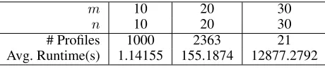
ILP for PUT-STV and Results.The solutions correspond to the elimination of a single alternative in each ofm−1
rounds and we test whether a given alternative is the PUT-winner by checking if there is a feasible solution when we enforce the constraint that the given alternative is not elim-inated in any of the rounds. We omit the details due to the space constraint. Table 4 summarizes the experimental
re-sults obtained using Gurobi’s ILP solver. Clearly, the ILP solver takes far more time than even our most basic search algorithms without improvements.
m 10 20 30
n 10 20 30
# Profiles 1000 2363 21
Avg. Runtime(s) 1.14155 155.1874 12877.2792
Table 4: ILP results for PUT-STV.
ILP for PUT-RP.We develop a novel ILP based on the char-acterization by Zavist and Tideman (Theorem 2). Let the in-duced weight(IW) between two verticesaandbbe the max-imum path weight over all paths fromatobin the graph. The path weight is defined as the minimum edge weight of a given path. An edge(u, v)isconsistentwith a rankingRif
uis preferred tovbyR.GRis a graph whose vertices areA and whose edges are exactly every edge in wmg≥0(P) con-sistent with a rankingR. Thus there is a topological ordering ofGRthat is exactlyR.
Example 3. In Figure 2, consider the induced weight from D toA in the bottom left graph. There are three distinct paths:P1 ={D →A},P2 ={D →C →A}, andP3=
{D → C → B → A}. The weight ofP1, orW(P1) = 1, W(P2) = 3and W(P3) = 1. Thus, IW(D, A) = 3, and note that IW(D, A)≥w(A,D)=−1.
Theorem 2. (Zavist and Tideman 1989) For any profile P and for any strict rankingR, the rankingR is the out-come of the ranked pairs procedure if and only ifGR
sat-isfies the following property for all candidates i, j ∈ A:
∀iRj, IW(i, j)≥w(j,i).
Based on Theorem 2, we provide a novel ILP formulation of the PUT-RP problem. See Appendices A.2 for details. Results. Out of1000 hard profiles, the RP ILP ran faster than DFS on16profiles. On these16profiles, the ILP took only41.097%of the time of the DFS to compute all PUT-winners on average. However over all1000 hard profiles, DFS is much faster on average: 29.131 times faster. We pro-pose that on profiles where DFS fails to compute all PUT-winners, or for elections with a large number of candidates, we can fall back on the ILP to solve PUT-RP.
7
Future Work
large profiles with many SCCs, since currently our dataset contains a low proportion of multi-SCC profiles. Also, we want to extend our search algorithm to multi-winner voting rules like the Chamberlin–Courant rule, which is known to be NP-hard to compute an optimal committee for general preferences (Procaccia, Rosenschein, and Zohar 2007).
8
Acknowledgments
We thank all anonymous reviewers for helpful comments and suggestions. This work is supported by NSF #1453542 and ONR #N00014-17-1-2621.
A
Appendices
A.1
Proof of Theorem 1
Suppose H = (A, E) is composed of SCCs Si (i =
1,· · · , k), and the set of bridge edgesB. We need to prove
C = (A, B ∪Sk
i=1Ci) is a maximal child of H, where
Ci is one of the maximal children ofSi. Suppose for con-tradiction that C is not one maximal child of H. From Lemma 1 we have thatCis acyclic. then it suffice that∃e∈
E\B∪Sk
i=1Ci
=B∪Sk
i=1Si
\B∪Sk
i=1Ci
=
Sk
i=1Si\Ci, s.t.{e} ∪B∪S k
i=1Ciis still acyclic. W.l.o.g., let’s assumee∈S1\C1. So{e} ∪C1is acyclic. But this contradicts the fact thatC1is a maximal child ofS1, since by definition,∀e0∈S
1\C1,C1∪ {e0}is cyclic.
Lemma 1. For any directed graphH = (A, E), composed of strongly connected componentsSi (i = 1,· · · , k), and
the set of bridge edgesB, the directed graphG= (A, B∪
Sk
i=1Ci)is also acyclic, whereCi is one of the maximal
children ofSi.
A.2
ILP Formulation for PUT-RP
We can test whether a given alternativei∗is a PUT-RP
win-ner if there is a solution subject to the constraint that there is no path from any other alternative toi∗. The variables are: (i) A binary indicator variableXi,jt of whether there is an
i → j path using locked in edges from ST
i≤t, for each
i, j ≤ m, t ≤ K. (ii) A binary indicator variableYt i,j,kof whether there is ani→kpath involving nodejusing locked in edges from tiersST
i≤t, for eachi, j, k≤m, t≤K.
We can determine all PUT-winners by selecting every al-ternativei∗ ≤m, adding the constraintP
j≤m,j6=i∗Xj,iK∗= 0, and checking the feasibility with the constraints below: •To enforce Theorem 2, for every pairi, j ≤m, such that
(j, i)∈Tt, we add the constraintXt
i,j≥Xi,jK.
•In addition, we have constraints to ensure that (i) locked in edges fromS
t≤KTtinduce a total order overAby enforc-ing asymmetry and transitivity constraints onXK
i,jvariables, and (ii) enforcing that ifXt
i,j= 1, thenX
ˆ
t>t i,j = 1.
•Constraints ensuring maximum weight paths are selected:
∀i, j, k≤m, t≤K,
Yt i,j,k≥X
t
i,j+Xj,kt −1
Yt i,j,k≤
Xi,jt +Xj,kt
2
i→j→k
∀i, k≤m, t≤K,
if(i, k)∈Etˆ≤t,Xi,kt ≥Xi,kK
(i, k)
∀j≤m,
Xi,kt ≥Yi,j,kt , if(i, k)∈Tˆt>t, Xt
i,k≤
P
j≤mYi,j,kt , if(i, k)∈Tˆt≤t, Xt
i,k≤
P
j≤mY t
i,j,k+Xi,kK
i→k
References
Brandt, F., and Geist, G. C. C. 2015. Pnyx: A Powerful and User-friendly Tool for Preference Aggregation. InProceedings of the 2015 International Conference on Autonomous Agents and Multi-agent Systems, 1915–1916.
Brill, M., and Fischer, F. 2012. The Price of Neutrality for the Ranked Pairs Method. InProceedings of the National Conference on Artificial Intelligence (AAAI), 1299–1305.
Conitzer, V.; Davenport, A.; and Kalagnanam, J. 2006. Improved bounds for computing Kemeny rankings. InProceedings of the National Conference on Artificial Intelligence (AAAI), 620–626. Conitzer, V.; Rognlie, M.; and Xia, L. 2009. Preference func-tions that score rankings and maximum likelihood estimation. In
Proceedings of the Twenty-First International Joint Conference on Artificial Intelligence (IJCAI), 109–115.
Csar, T.; Lackner, M.; Pichler, R.; and Sallinger, E. 2017. Winner Determination in Huge Elections with MapReduce. InProceedings of the AAAI Conference on Artificial Intelligence.
Freeman, R.; Brill, M.; and Conitzer, V. 2015. General Tiebreaking Schemes for Computational Social Choice. InProceedings of the 2015 International Conference on Autonomous Agents and Multi-agent Systems, 1401–1409.
Kenyon-Mathieu, C., and Schudy, W. 2007. How to Rank with Few Errors: A PTAS for Weighted Feedback Arc Set on Tourna-ments. InProceedings of the Thirty-ninth Annual ACM Symposium on Theory of Computing, 95–103.
Kleinberg, J., and Tardos, E. 2005.Algorithm Design. Pearson. Mattei, N., and Walsh, T. 2013. PrefLib: A Library of Preference Data. InProceedings of Third International Conference on Algo-rithmic Decision Theory (ADT 2013), Lecture Notes in Artificial Intelligence.
Mattei, N.; Narodytska, N.; and Walsh, T. 2014. How Hard Is It to Control an Election by Breaking Ties? InProceedings of the Twenty-first European Conference on Artificial Intelligence, 1067– 1068.
McGarvey, D. C. 1953. A theorem on the construction of voting paradoxes.Econometrica21(4):608–610.
O’Neill, J. 2011. https://www.opavote.com/methods/single-transferable-vote.
Procaccia, A. D.; Rosenschein, J. S.; and Zohar, A. 2007. Multi-winner elections: Complexity of manipulation, control and Multi- winner-determination. InIJCAI, volume 7, 1476–1481.
Schulze, M. 2011. A new monotonic, clone-independent, re-versal symmetric, and Condorcet-consistent single-winner election method.Social Choice and Welfare36(2):267—303.
Tideman, T. N. 1987. Independence of clones as a criterion for voting rules.Social Choice and Welfare4(3):185–206.
Wikipedia. 2018. Single transferable vote — Wikipedia, the free encyclopedia. [Online; accessed 30-Jan-2018].
Zavist, T. M., and Tideman, T. N. 1989. Complete independence of clones in the ranked pairs rule. Social Choice and Welfare