The Thirty-Third AAAI Conference on Artificial Intelligence (AAAI-19)
Running Time Analysis of MOEA/D with
Crossover on Discrete Optimization Problem
Zhengxin Huang,
1Yuren Zhou,
1,2,∗Zefeng Chen,
1Xiaoyu He
11School of Data and Computer Science, Sun Yat-Sen University, Guangzhou 510006, China
2Engineering Research Institute, Guangzhou College of South China, University of Technology, Guangzhou 510800, China
Email: [email protected], [email protected], [email protected], [email protected]
Abstract
Decomposition-based multiobjective evolutionary algorithms (MOEAs) are a class of popular methods for solving multiob-jective optimization problems (MOPs), and have been widely studied in numerical experiments and successfully applied in practice. However, we know little about these algorithms from the theoretical aspect. In this paper, we present a running time analysis of a simple MOEA with crossover based on the MOEA/D framework (MOEA/D-C) on four discrete op-timization problems. Our rigorous theoretical analysis shows that the MOEA/D-C can obtain a set of Pareto optimal so-lutions to cover the Pareto front of these problems in ex-pected running time apparently lower than the one without crossover. Moreover, the MOEA/D-C only needs to decom-pose an MOP into a few scalar optimization subproblems ac-cording to several simple weight vectors. This result suggests that the use of crossover in decomposition-based MOEA can simplify the setting of weight vector for different problems and make the algorithm more efficient. This study theoreti-cally explains why some decomposition-based MOEAs work well in computational experiments and provides insights in design of MOEAs for MOPs in future research.
Introduction
Multiobjective optimization problem (MOP) involves the si-multaneous optimization of multiple conflicting objectives. It exists widely in real-world applications (Zhou et al. 2011). The goal of multiobjective optimization is to find a set of the best eclectic solutions called the Pareto optimal solu-tions. Due to the advantage of population-based nature, evo-lutionary algorithms (EAs) are able to obtain multiple Pareto optimal solutions in a single run, and multiobjective EAs (MOEAs) have been very popular in solving MOPs. MOEAs are broadly classified into three categories, i.e., domination-based, indicator-based and decomposition-based (Trivedi et al. 2017). In this paper, we present a theoretical analy-sis of a simple decomposition-based MOEA with crossover (MOEA/D-C) on several discrete optimization problems.
The idea of decomposition for solving MOPs has been used in (Ishibuchi and Murata 1998; Murata and Gen 2002). However, it becomes popular after the MOEA/D framework is presented in (Zhang and Li 2007). In this framework,
Copyright c2019, Association for the Advancement of Artificial Intelligence (www.aaai.org). All rights reserved.
an MOP is first decomposed into some scalar optimization subproblems according to the decomposition approach and weight vector. Then all subproblems are solved simultane-ously by employing an EA. In the past decade, there are vast studies that have contributed to improving and developing MOEAs based on the MOEA/D framework, e.g., studies on novel weight vector generation methods (Qi et al. 2014; Gi-agkiozis, Purshouse, and Fleming 2014), improved decom-position approaches (Ishibuchi et al. 2010; Wang, Zhang, and Zhang 2016) and selection mechanisms (Chiang and Lai 2011; Li et al. 2017). For further decomposition-based MOEAs, the readers are advised to (Trivedi et al. 2017).
In (Ishibuchi et al. 2017), the authors conducted an exper-imental analysis for MOEAs based on the MOEA/D frame-work on the DTLZ and WFG test problems. Their results show that the performance of the algorithm strongly depends on Pareto front shapes. In (Tanabe and Ishibuchi 2018), the authors presented a parameter study in the MOEA/D frame-work using the unbounded external archive (UEA). Their ex-perimental results indicate that suitable settings of the three control parameters (population size, scalarizing functions and penalty parameter of the penalty-based boundary inter-section (PBI) function) significantly depend on the choice of UEA scenarios. An experimental study on the effect of refer-ence point in the MOEA/D framework for optimizing WFG test problems is presented in (Wang et al. 2017). Their exper-imental results show that different reference point specifica-tions lead to different performance of exploitation and ex-ploration, and the strategy of dynamic reference point spec-ifications is recommended to use for unknown problems.
obtained by using the evenly distributed generation method. This explains why an optimally decomposed weight vector is hard to obtain for different MOPs in practical applications. Crossover operator often plays an important role in the search process of EAs and is widely used in numerical ex-periments. However, comparing to the mutation operator, the understanding of the effect of the crossover operator in EAs from theoretical analysis aspect is limited (Sudholt 2017). There are several studies have contributed to this issue. For single optimization problems, these researches (Jansen and Wegener 2002; K¨otzing, Sudholt, and Theile 2011; Lehre and Yao 2011; Doerr et al. 2013; Doerr, Do-err, and Ebel 2015; Sudholt 2017; Doerr and Doerr 2018; Dang et al. 2018) have shown that crossover operator can speed up the search. Specifically, they proved that EAs enabled crossover outperform the disabled ones on some benchmark discrete optimization problems in term of the ex-pected running time. As far as we know, the first running time analysis to show that the helpfulness of crossover on MOP is presented in (Neumann and Theile 2010). In (Qian, Yu, and Zhou 2013), the authors presented a running time analysis to show that crossover leads to better upper bounds than previous known result for LPTNO (LOTZ) and COCZ problems. These results indicate that crossover is helpful for EAs on optimizing some problems. However, whether it does help for decomposition-based MOEAs on optimizing MOPs has not yet been investigated from theoretical aspect. In this paper, we present a running time analysis of a sim-ple decomposition-based MOEA with crossover (MOEA/D-C) on four benchmark discrete optimization problems, i.e., COCZ, LPTNO, Dec-obj-MOP and Plateau-MOP. The up-per bounds of expected running time obtained by MOEA/D-C are lower than the MOEA/D-M an order ofn, wherenis the size of decision variable. These bounds are better than or at least the best known ones. Moreover, there is an in-teresting thing worth mentioning that the MOEA/D-C only needs to decompose these MOPs instances into several sub-problems according to a set of simple weight vectors while the MOEA/D-M needs to findΘ(n)optimally decomposed weight vectors. This theoretical study reveals that the use of crossover operator in MOEA/D framework can simplify the setting of weight vectors for different problems and make the algorithm more efficient. It provides insights in the design of decomposition-based MOEAs for MOPs in future research.
Algorithm and Problem
Analyzed Algorithm
An MOP can be formally defined as follows:
max F(x) = f1(x),· · ·, fm(x)
s.t. x∈X, (1)
whereXis the decision space andx= (x1,· · ·, xn)is the
decision variable,F : X → Rm consists of mfunctions
andRmis the objective space. Since themobjectives of (1)
are often mutually conflicting, there is no a solutionxthat can maximize all objectives simultaneously. Instead, these conflicting objectives give rise to a set of eclectic optimal solutions. Forx1, x2 ∈ X, we say that x1 dominates x2,
denoted asx1 x2, if and only iffi(x1)≥fi(x2)for all
i= 1,· · · , mandfi(x1)> fi(x2)for at least one indexi.
A solutionx∗ ∈X is Pareto optimal if there is no solution xsuch thatxx∗. The set of all Pareto optimal solutions is calledPareto optimal set(PS) and the set of all objective vectors corresponding to PS is called thePareto front(PF).
In the MOEA/D framework, an MOP is decomposed into some scalar optimization subproblems according to the de-composition approach and weight vectors. As in the first im-plemented algorithm of the MOEA/D framework in (Zhang and Li 2007), the Tchebycheff decomposition approach and simplex-lattice weight vector generation method are used in MOEA/D-C as well as in the MOEA/D-M. Given an MOP defined in (1), the scalar optimization subproblem generated by the Tchebycheff approach is
min g(x|λ) = max
1≤i≤m{λi|fi(x)−z
∗
i|}
s.t. x∈X,
(2)
whereλ = (λ1,· · ·, λm)is the weight vector, i.e.,λi ≥ 0
fori= 1,· · · , mandPmi=1λi= 1, andz∗= (z∗1,· · ·, z∗m)
denotes the reference point, i.e.,z∗i = max{fi(x)|x∈X}.
By altering the weight vector, the Tchebycheff approach generates different scalar optimization subproblems in form of (2) for an MOP defined in (1). LetHbe a positive integer. The simplex-lattice design method generates weight vectors by takingmvalues from{0/H,1/H,· · · , H/H}such that
Pm
i=1λi = 1. Thus, for an MOP withm objectives and
integerH, there areN =CHm+−m1−1weight vectors, and each one corresponds to a scalar optimization subproblem.
After decomposition, for each subproblem the MOEA/D framework first selects theTclosest subproblems to form its neighbor set, whereT is an input parameter calledneighbor size. The distance are measured by the Euclidean distance between their weight vectors. It then controls a population of sizeN to cooperatively solve theN scalar optimization subproblems by using the neighborhood-based coevolution. A description of the presented MOEA/D-C is given in Al-gorithm 1. Different from the MOEA/D-M only using muta-tion to create the offspring, the MOEA/D-C allows to use the crossover operator in Step 7. Observe that the important de-composition and neighborhood-based coevolution features of the MOEA/D framework are retained in Algorithm 1.
Analyzed Problems
We denote bykxk1the number of 1-bits in solutionx. The
four analyzed MOPs in this paper are defined as follows.
Definition 1 (COCZ). The pseudo-Boolean function
COCZ:{0,1}n→
N2is defined as follows:
COCZ(x) = kxk1, n− kxk1
.
This instance is an extension of the COUNTONES prob-lem called count ones count zeroes (COCZ). The above def-inition of COCZ is used in (Li et al. 2016), which is lightly different from the definition in (Laumanns, Thiele, and Zit-zler 2004). However, this change does not effect the run-ning time analysis since it only extends the size of PF from
Algorithm 1MOEA/D-C
Input:An MOP withmobjectives, stop criterion, param-eter H, the number of scalar optimization subproblems N, weight vectors{λ1,· · ·, λN}and neighbor sizeT. Output:A Pareto optimal solution setP.
1: Initialization: The Pareto optimal solution setP = ∅.
For each subproblem g(x|λk), k = 1,· · · , N, select
theT closest subproblems into its neighbor setBk
ac-cording to the Euclidean distance between their weight vectors. Generate a solutionxk ∈ {0,1}nuniformly at
random for each subproblemg(x|λk). Set the reference
pointz = (z1,· · ·, zm), wherezi = max{fi(xk)}for
k= 1,· · ·, N. LetSkdenote the set of solutions
corre-sponding to subproblems inBk. 2: whilestop criterion is not satisfieddo
3: foreach subproblemg(x|λk),k= 1,· · ·, Ndo 4: ifrand > pcthen
5: Create two new solutionsx0k, x00kfor thekth sub-problem by using the mutation operator toxk. 6: else
7: Create two new solutionsx0k, x00kfor thekth sub-problem by using the crossover operator onxk
and a solution inSk\xk. 8: end if
9: Updatez:for eachzi, ifmax{fi(x0k), fi(x00k)} >
zi, setzi= max{fi(x0k), fi(x00k)},i= 1,· · ·, m.
10: Update Sk: for each solution xj in Sk, if
min{g(x0k|λj), g(x00
k|λj)} ≤ g(xj|λj), replacexj
with the better one in{x0
k, x00k}.
11: UpdateP:remove all solutions dominated byx0k
orx00k fromP. Ifx0korx00k is not dominated by so-lutions inP, add it intoP.
12: end for
13: end while
expected running time. A similar definition of this instance called ONEMINMAXis presented in (Giel and Lehre 2010). All solutions of COCZ are Pareto optimal and the distribu-tion of elements in the PF is shown in Figure 1 (red points). Definition 2 (WLPTNO). The pseudo-Boolean function
W LP T N O:{−1,1}n→
R2is defined as follows:
W LP T N O(x) =
n X
i=1
wi i Y
j=1
(1 +xi), n X
i=1
vi n Y
j=i
(1−xi)
,
wherewi, vi>0fori= 1,· · ·, n.
This instance is defined in (Qian, Yu, and Zhou 2013). The abbreviation WLPTNO stands for Weighted Leading
Posi-tive Ones Trailing NegaPosi-tive Ones. It can be considered as
an extension of LOTZ (Leading Ones Trailing Zeroes) by shifting the decision space from{0,1}n to{−1,1}n, and
adding weightswi andvifor each leading positive one and
trailing negative one bits, respectively. However, it mostly has very different properties from LOTZ. As in analyzing the MOEA/D-M (Li et al. 2016), we setwi =vi = 1and
denote this case as LPTNO. Note that the obtained upper bound of the expected running time in this paper is also true
for other setting of weights. The PS of LPTNO hasn+1 ele-ments. As shown in Figure 2, unlike the COCZ, the elements of the PF are not evenly distributed.
f1
0 5 10 15 20 25
f2
0 5 10 15 20 25
COCZ Plateau-MOP
Figure 1: Pareto front of the COCZ withn= 25and Plateau-MOP withn= 20.
f1 ×106
0 0.5 1 1.5 2 2.2
f2 ×106
0 0.5 1 1.5 2 2.2
f1 ×104
0 1 2 3 4
f2 ×104
0 1 2 3 4
Figure 2: Pareto front of the LPTNO withn= 20.
Definition 3(Dec-obj-MOP). The pseudo-Boolean function
Dec–obj–M OP :{0,1}n→
N2is defined as follows:
Dec–obj–M OP(x) = f1(x), f2(x),
where
f1(x) =n+ 1− kxk1 mod (n+ 1),
f2(x) =n+kxk1 mod (n+ 1).
This instance is defined in (Li et al. 2016). There is de-ceptive property in the search space of f2. The location of
the global optimum is very far from the local optimum in the search space, and the fitness-based search will be mostly guided to the local optimum. Thus, these kinds of functions are deceptive and hard to solve. The expected running time to obtain the optimal solution for some subproblems of Dec-obj-MOP is Ω(nn)(Li et al. 2016). The PS and the PF of
Dec-obj-MOP are the same as the COCZ.
Definition 4(Plateau-MOP). Let1i0n−i denote that there
areileading ones andn−itrailing zeroes in the solutionx.
The pseudo-Boolean functionP lateau–M OP :{0,1}n →
N2is defined as follows:
P lateau–M OP(x) = f1(x), f2(x)
,
where
f1(x) =
n ifx= 1n,
3n/4 ifx= 1i0n−i,3n/4< i < n, i ifx= 1i0n−i,0≤i≤3n/4,
f2(x) = n
−i ifx= 1i0n−i,0≤i≤n,
−kxk1 otherwise.
This instance is defined in (Li et al. 2016). For conve-nience, we hereafter assume that n4 is integral. Although neither objective functions in Plateau-MOP is deceptive, it is hard to solve for SEMO. The expected running time of SEMO on Plateau-MOP isΩ(n0.25n)(Li et al. 2016).
Forf1, there is a plateau whichxis in form of1i0n−ifor
i∈[34n, n−1]. So solutions of Plateau-MOP in this range are dominated by the solution 13n/40n/4 since the fitness
value off2 becomes worse with increasing kxk1. The PS
of Plateau-MOP has 34n+ 2elements, which are1i0n−ifor
i∈ {[0,34n]} ∪ {n}. The elements on PF of Plateau-MOP is
shown in Figure 1 (blue points). Note that the point(n,0)is an outlier in the objective space.
Running Time Analysis
In this section, we present the running time analysis of gorithm 1 on the four above MOPs. For parameters in Al-gorithm 1, in this analysis we set H = 2, T = m and pc = 0.5. So the set of decomposed weight vectors is
{λ1 = (0,1), λ2 = (0.5,0.5), λ3= (1,0)}and the number
of scalar optimization subproblemsN (also the population size) is 3. For the variation operators in Step 5 and 7, we use the standard bit mutation and one-point crossover, respec-tively. Thus Algorithm 1 requires six fitness evaluations in an iteration. For ease of expression, we assume that the op-timal value of each objective for these problems have been known in the following analysis. Note that this assumption does not effect the expected running time of Algorithm 1 on these problems, because in each iteration any new solution with better fitness value for the objective will be updated immediately in Step 9 and can be accepted in Step 10.
Analysis on COCZ
For COCZ, a set of Pareto optimal solutions corresponding to the PF is{0n,0∗n−11∗,· · · ,1n}, where0∗i1∗j indicates
that there arei0-bits andj1-bits randomly distributed in the solution. The best known upper bound of expected running time on COCZ is O(nlogn)(Qian, Yu, and Zhou 2013). In (Li et al. 2016), the authors proved that the evenly dis-tributed weight vectors, i.e.,λk= (λk1,1−λk1), λk1= kn, k=
0,· · · , n, producen+ 1subproblems that are mapped
one-to-one to the points in the PF. So the MOEA/D-M with H = nobtains a set of solutions to cover the PF by solv-ing then+ 1subproblems. Thus, the expected running time of the MOEA/D-M on COCZ isO(n2logn)since it solves each subproblem in expected running timeO(nlogn).
These decomposed subproblems for COCZ in Algorithm 1 (Tchebycheff approach) are listed as follows:
min g(x|λ1) =kxk1, (3)
min g(x|λ2) = max{0.5(n− kxk1),0.5kxk1}, (4)
min g(x|λ3) =n− kxk1. (5)
In the following, we prove that the expected running time of Algorithm 1 on COCZ isO(nlogn). The analysis con-sists of two phases. In the first phase, by neglecting the pro-motion of the crossover operator and coevolution, we prove
that Algorithm 1 can find an optimal solution for each sub-problem by using the mutation operator in expected running timeO(nlogn). In the second phase, we prove that by us-ing the crossover operator to optimal solutions for the three subproblems, Algorithm 1 obtains a set of solutions to cover the PF in expected running timeO(nlogn).
Lemma 1. For COCZ, Algorithm 1 finds an optimal solution
for each subproblem in expected running timeO(nlogn).
Proof. The optimization process of these functions is
simi-lar to optimize the well-known ONEMAXfunction. For (3) (or (5)), the fitness value becomes better when increasing the 0-bits (1-bits) in solution x and the optimal solution is 0n (1n). Let i denote the number of 0-bits (1-bits) in the current solution. For Algorithm 1, the mutation opera-tor produces a better solution for (3) (or (5)) from the cur-rent one with probability (n−2i) · 1
n ·(1− 1 n)
n−1 ≥ n−i 2en,
since it happens if one of these 0-bits (1-bits) is flipped while keeping other bits unchanged. Recall thatpc = 0.5.
Thus, according to the fitness level approach (Sudholt 2013; Jansen 2013), Algorithm 1 finds the optimal solution for (3) and (5) in expected running time O(nlogn). For (4), the optimal solution0∗n/21∗n/2is close to the initial solution.
Ifkxk1 < 0.5n, the fitness value becomes better when
in-creasingkxk1. Ifkxk1>0.5n, decreasingkxk1will lead to
a better fitness value. Thus, Algorithm 1 finds a better solu-tion for (4) in an iterasolu-tion with probability at least n2en−i and the expected running time isO(nlogn).
Theorem 1. For COCZ, Algorithm 1 obtains a set of
solu-tions to cover the PF in expected running timeO(nlogn).
Proof. Since each subproblem selects two closest
subprob-lems intoBk according to the Euclidean distance between
their weight vectors, we haveS1={0n,0∗n/21∗n/2},S2=
{0∗n/21∗n/2,0nor1n} and S3 = {1n,0∗n/21∗n/2} after
solutions 0n,0∗n/21∗n/2 and1n have been found for (3),
(4) and (5), respectively. Thus, the rest of Pareto solutions corresponding to PF can be partitioned into two disjoint sets, i.e.,R1={0∗n−11∗1,0∗n−21∗2,· · ·,0∗n/2+11∗n/2−1}and
R2 = {0∗n/2−11∗n/2+1,0∗n/2−21∗n/2+2,· · · ,0∗11∗n−1}.
In the following, we show that those solutions produced by using crossover operator on solutions inS1andS3coverR1
andR2 in expected running time O(nlogn), respectively.
Note that solutions produced by using crossover operator on solutions inS2and mutation operator to the three solutions
during this phase can only accelerate the search process. In each iteration, Algorithm 1 applies crossover to solu-tions inS1andS3with probabilitypc= 0.5. Note that there
are 0.5n 1-bits in solution 0∗n/21∗n/2 and the crossover point is selected from 1 to n−1 uniformly. Letl1 andl2
denote the position of the first and the last 1-bit in solution
0∗n/21∗n/2. We havel
2−l1 ≥ 0.5n. We call a crossover
a success if it produces solutions inR1and at least one of
them have not been produced in previous crossovers. ForS1,
if the crossover point is located in(l1, l2), it produces two
solutions inR1since the other solution inS1is0n. Hence,
of solutions to coverR1because each success produces two
new solutions inR1and|R1|= 0.5n−1. Observe that there
are one or two points in(l1, l2)corresponding to each
suc-cess. Thus, a success happens in an iteration with probability at least02(.25n−n−1)i, whereidenotes the number of successes so far. Therefore, the expected running time of Algorithm 1 ob-tained a set of solutions to coverR1is upper bounded by
0.25n−1 X
i=0
2(n−1)
0.25n−i ≤2n
0.25n X
j=1
1
j =O(nlogn).
Similarly, we have that Algorithm 1 obtains a set of solutions to coverR2in expected running timeO(nlogn).
Therefore, combined with Lemma 1, Algorithm 1 obtains a set of solutionsSto cover the whole PF, i.e.,P F ⊆F(S), of COCZ in expected running timeO(nlogn).
Analysis on LPTNO
For LPTNO, the set of Pareto optimal solutions correspond-ing to the PF is{1n,1n−1(−1),· · · ,(−1)n}, and the best
known upper bound of expected running time is O(n2)
(Qian, Yu, and Zhou 2013). In (Li et al. 2016), the authors proved that the weight vectors, λk = (λk1,1−λk1), λk1 =
Pk j=12
n+1−j
Pn j=k+12j+
Pk
j=12n+1−j
, k = 0,· · · , n, produces a set of
subproblems which are mapped one-to-one to the points in the PF. So the MOEA/D-M with H = nobtains a set of solutions to cover the PF by solving the decomposed n+ 1subproblems. Thus, the expected running time of the MOEA/D-M on LPTNO isO(n3)since it solves each
sub-problem in expected running timeO(n2). Note that this set
of weight vectors are not evenly distributed since most ofλk fall nearby(0.5,0.5).
These decomposed subproblems for LPNTO in Algo-rithm 1 (Tchebycheff approach) are listed as follows:
min g(x|λ1) =2n+1−2−
n X
i=1 n Y
j=i
(1−xi), (6)
min g(x|λ2) = max2n−1−0.5
n X
i=1 i Y
j=1
(1−xi),
2n−1−0.5
n X
i=1 n Y
j=i
(1 +xi) , (7)
min g(x|λ3) =2n+1−2−
n X
i=1 i Y
j=1
(1 +xi). (8)
Lemma 2. For LPTNO, Algorithm 1 finds the optimal
solu-tion for each subproblem in expected running timeO(n2).
Proof. The optimization process of functions (6), (7) and
(8) is similar to optimize the well-known LEADINGONES
function. For (8) (or (6)), the fitness value becomes bet-ter when increasing the leftmost 1-bits (rightmost (−1 )-bits) in x and the optimal solution is 1n ((−1)n). So in Algorithm 1 the mutation operator produces a better solu-tion for (8) (or (6)) from the current one with probability
1 2·
1 n·(1−
1 n)
n−1≥ 1
2en, because its fitness value will
de-crease when the leftmost (−1)-bit (rightmost 1-bit) is flipped while keeping other bits unchanged. Thus, according to the fitness level approach, the expected running time of Algo-rithm 1 to find the optimal solution for (8) (or (6)) isO(n2)
since there are at mostnbits to be flipped. For (7), any new solution where the minimum number of leading 1-bits and trailing (−1)-bits is non-decreased is accepted in the itera-tion. If the optimal solution is not found, there must exist at least a bit which is flipped to produce an accepted solution, and thus a new solution is accepted with probability at least
1
2en. Note that if the difference between the numbers of
lead-ing 1-bits and trilllead-ing (−1)-bits is 1, there is a small plateau, which consists of two points and needs at most additional ex-pected timeO(n)to leave since it needs two random walks on the plateau in expectation. Therefore, Algorithm 1 also finds the optimal solution1n/2(−1)n/2for (7) in expected
running timeO(n2).
Theorem 2. For LPTNO, Algorithm 1 obtains a set of
solu-tions to cover the PF in expected running timeO(n2).
Proof. Because Algorithm 1 selects two closest
sub-problems into Bk according to the Euclidean distance
between their weight vectors for each subproblem, we have that S1 = {(−1)n,1n/2(−1)n/2}, S2 =
{1n/2(−1)n/2,(−1)nor1n}andS
3 ={1n,1n/2(−1)n/2}
after solutions (−1)n,1n/2(−1)n/2 and 1n have been
found for subproblems (6), (7) and (8), respectively. The rest of Pareto optimal solutions corresponding to PF can be partitioned into two disjoint sets, that is,R1 =
{1(−1)n−1,12(−1)n−2,· · ·,1n/2−1(−1)n/2+1}andR2=
{1n/2+1(−1)n/2−1,1n/2+2(−1)n/2−2,· · · ,1n−1(−1)}.
We next show that those solutions produced by using crossover operator on solutions inS1andS3 coverR1and
R2in expected running timeO(nlogn), respectively.
For the two solutions inS1, the leftmost0.5n−1bits have
different value. If and only if one of these bits is selected, the crossover creates a unique solution inR1. Thus, to obtain a
set of solutions to cover R1, the crossover operator needs
to select each of these bits at least once. Let idenote the number of these bits that have been selected, a new bit is selected by the crossover in a new iteration with probability
0.5n−1−i
2(n−1) . Recall thatpc= 0.5. Thus, Algorithm 1 obtains a
set of solutions to coverR1in expected running time
0.5n−2 X
i=0
2(n−1)
0.5n−1−i ≤2n
0.5n X
j=1
1
j =O(nlogn).
Similarly, we have that Algorithm 1 obtains a set of solutions to coverR2in expected running timeO(nlogn).
Therefore, combined with Lemma 2, Algorithm 1 obtains a set of solutions to cover the whole PF of LPNTO in ex-pected running timeO(n2).
Analysis on Dec-obj-MOP
O(n2logn)(Li et al. 2016). The evenly distributed weight vectors, i.e., λk = (λk
1,1 −λk1), λk1 = k
n, k = 0,· · ·, n,
also produces a set of subproblems that are mapped one-to-one to the points in the PF. However, different from COCZ that every decomposed subproblems can be solved in ex-pected running timeO(nlogn), the expected fitness evalu-ations to find the optimal solution for the subproblem corre-sponding to weight vector(0,1), i.e., (9), isΩ(nn). But the expected running time of the MOEA/D-M on Dec-obj-MOP isO(n2logn), because the optimal solution for (9) can be
obtained and added intoPby other subproblems in expected running timeO(nlogn).
For Dec-obj-MOP, these decomposed subproblems in Al-gorithm 1 are listed as follows:
min g(x|λ1) =n−f2(x), (9)
min g(x|λ2) = max1
2{(n−f1(x)),(n−f2(x))}, (10)
min g(x|λ3) =n−f1(x), (11)
wheref1(x)andf2(x)are the same as in the Definition 3.
Lemma 3. For Dec-obj-MOP, Algorithm 1 finds an optimum for subproblems (10) and (11) and the local optimum for
subproblem (9) in expected running timeO(nlogn).
Proof. For (11), the fitness value becomes better when
de-creasingkxk1 ifkxk1 > 1. Thus, similar to optimize the
ONEMAX, starting from any uniformly random solution Algorithm 1 finds the optimal solution 0∗n−11∗ for (11) in expected running timeO(nlogn). For (10), the fitness value becomes better when increasingkxk1ifkxk1 <0.5n
and decreasingkxk1 ifkxk1 > 0.5n. Thus, starting from
any initial solution Algorithm 1 finds the optimal solution
0∗n/21∗n/2 for (10) in expected running time O(nlogn).
For (9), the optimal solution is0n. There is deceptive
prop-erty in the search space since the fitness value becomes bet-ter when increasingkxk1ifkxk1 > 0. Since the expected
number of 1-bits in an initial solution is n2 > 0, by Cher-noff bound, the search will be guided to the solution1nwith
probability1−e−Ω(n). Thus, Algorithm 1 finds the local
op-timum1nfor (9) in expected running timeO(nlogn).
Although the mutation operator cannot find the optimal solution for (9) in polynomial running time, we next show that Algorithm 1 still obtains a set of solutions to cover the PF of Dec-obj-MOP in expected running timeO(nlogn).
Theorem 3. For Dec-obj-MOP, Algorithm 1 obtains a set of solutions to cover the PF in expected running time
O(nlogn).
Proof. For Dec-obj-MOP, we haveS1={1n,0∗n/21∗n/2},
S2 = {0∗n/21∗n/2,1nor0∗n−11∗} and S3 =
{0∗n−11∗,0∗n/21∗n/2} after solutions 1n,0∗n/21∗n/2
and0∗n−11∗have been found for subproblems (9), (10) and (11), respectively. We partition the rest of Pareto optimal solutions corresponding to PF into three disjoint sets, i.e., R1 = {0∗n/2−11∗n/2+1,0∗n/2−21∗n/2+2,· · · ,0∗11∗n−1},
R2 = {0∗n−21∗2,0∗n−31∗3,· · ·,0∗n/2+11∗n/2−1} and
R3={0n}.
Since solutions produced by using crossover on solutions inS1 are the same as the case in COCZ that each success
creates two new solutions inR1, Algorithm 1 obtains a set of
solutions to coverR1in expected running timeO(nlogn).
ForR2, there is a bit difference with the case in COCZ,
because there is a 1-bit in the solution0∗n−11∗∈S3and it
will be copied into an offspring in the one-point crossover. In such way, some successes may only produce a new so-lution in R2 since the other one is a duplication of
previ-ous solutions. Thus, forS3the crossover operator may take
0.5n−2successes to obtain a set of solutions to coverR2
since|R2| = 0.5n−2. Observe that there is at least one
point in (l1, l2) corresponding to a success, where l1 and
l2 denote the position of the first and the last 1-bit in the
solution 0∗n/21∗n/2. For Algorithm 1, the probability of a
success happening in an iteration is 0.2(5nn−−21)−i, where i de-notes the number of successes so far. Recall thatpc = 0.5.
Thus, the expected running time of the crossover operator produced a set of solutions to coverR2is upper bounded by
0.5n−3 X
i=0
2(n−1)
0.5n−2−i ≤2n
0.5n X
j=1
1
j =O(nlogn).
For the solution 0n inR
3, it may be created by using
crossover operator to solutions inS2 andS3. However, the
probability of this event is complex to compute and the lower bound seems to be very small. We next show that it can still be found by Algorithm 1 in expected running time O(n). Note that after the optimal solution0∗n−11∗has been found for (11), it will be kept by this subproblem forever. Thus, in later mutations it will be always used to create an offspring, and the offspring is0n with probability at least 1
en since it
happens when the 1-bit is flipped and all 0-bits are kept un-changed. Thus, the solution0nis created and added intoP by the mutation operator in expected running timeO(n).
Therefore, combined with Lemma 3, Algorithm 1 obtains a set of solutions to cover the PF of Dec-obj-MOP in ex-pected running timeO(nlogn).
Analysis on Plateau-MOP
The PF of Plateau-MOP is{(0, n),(1, n−1),· · · ,(3n/4, n/4),(n,0)}and the set of Pareto optimal solutions corre-sponding to PF is{0n,10n−1,· · ·,13n/40n/4,1n}. The best
known upper bound of expected running time on Plateau-MOP is O(n3) (Li et al. 2016). The evenly distributed weight vector, i.e., λk = (λk
1,1 − λk1), λk1 = k n, k =
0,· · · , n, produces a set of subproblems that are mapped
one-to-one to the points on PF. So MOEA/D-M withH =n finds a set of solutions to cover the PF by solving the decom-posedΘ(n)subproblems. Thus, the expected running time of MOEA/D-M on Plateau-MOP (exclude the outlier point
(n,0)) isO(n3)since it solves each subproblem in expected running timeO(n2)(Li et al. 2016).
Al-gorithm 1 are listed as follows:
min g(x|λ1) =n−f2(x), (12)
min g(x|λ2) = max1
2{(n−f1(x)),(n−f2(x))}, (13)
min g(x|λ3) =n−f1(x), (14)
wheref1(x)andf2(x)are the same as in the Definition 4.
Lemma 4. For Plateau-MOP, Algorithm 1 finds the optimal solution for subproblems (12) and (13) and a suboptimal
so-lution for subproblem (14) in expected running timeO(n2).
Proof. For (12), starting from any initial solutionx, the
op-timization process first tries to minimize the 1-bits in it or directly jump to a solution with form of1i0n−i, then it tries
to flip the rightmost 1-bit into 0-bit until the optimal solu-tion 0n is found. The first part is equivalent to optimizing
the ONEMAX(O(nlogn)) and the second part is equivalent to optimizing the LEADINGONES(O(n2)). Thus, Algorithm
1 finds the optimal solution for (12) in expected running time O(n2). For (13), the optimal solution is1n/20n/2. First, by
Chernoff bound, we have that any initial solution turns into the form of 1i0n−i in expected running time O(nlogn),
wherei ≤ 3n
4 with probability 1−e
−Ω(n). Second, from
any solution in form of1i0n−i for i ≤ 3n
4, the fitness
be-comes better when increasingiifi < 0.5nand decreasing iifi > 0.5n, which happens with probability at least en1. Thus, Algorithm 1 finds the optimal solution1n/20n/2for (13) in expected running timeO(n2). For (14), in the
objec-tive space there is a plateau (suboptimal solutions), which is in form of1i0n−i fori ∈ [3
4n, n−1]. Thus, Algorithm 1
finds the suboptimal solution13n/40n/4in expected running
timeO(n2)from any solution in form of1i0n−i. After
find-ing the suboptimal solution13n/40n/4, it randomly walks on
the plateau and accepts any new solution which is in form of
1i0n−iwithi≥ 3 4n.
Theorem 4. For Plateau-MOP, Algorithm 1 obtains a set of solutions to cover the PF (except the outlier point) in
ex-pected running timeO(n2).
Proof. After Algorithm 1 finds the optimal solution for
subproblems (12) and (13) and a suboptimal solution for (14) (assume that is 13n/40n/4 for convenience), we have
S1 = {0n,1n/20n/2},S2 = {1n/20n/2,0nor13n/40n/4}
and S3 = {13n/40n/4,1n/20n/2}. Thus, except the
out-lier point, the rest of Pareto optimal solutions correspond-ing to PF can be partitioned into two disjoint sets, that is,R1 = {1n/2−10n/2+1,1n/2−20n/2+2,· · ·,10n−1} and
R2={1n/2+10n/2−1,1n/2+20n/2−2,· · · ,13n/40n/4}.
For the two solutions inS1, the leftmost0.5n−1bits have
different value. If and only if one of these bits is selected, the crossover creates a unique solution inR1. Thus, to obtain a
set of solutions to coverR1, the crossover phase needs to
select each of these bits once. Leti denote the number of these bits that have been selected, a new bit is selected by the crossover operator in the next iteration with probability
0.5n−1−i
2(n−1) . Recall thatpc = 0.5. Thus, the expected running
time of Algorithm 1 obtained a set of solutions to coverR1
is upper bounded by
0.5n−2 X
i=0
2(n−1)
0.5n−1−i ≤2n
0.5n X
j=1
1
j =O(nlogn).
Similarly, forR2there aren4 Pareto optimal solutions, and a
new solution is created in an iteration by applying crossover on solutions in S3with probability 02(.25n−n−1)i. Thus, we also
have that Algorithm 1 obtains a set of solutions to coverR2
in expected running timeO(nlogn).
Therefore, combined with Lemma 4, Algorithm 1 obtains a set of solutions to cover the PF (except the outlier point) of Plateau-MOP in expected running timeO(n2).
Experimental Verification
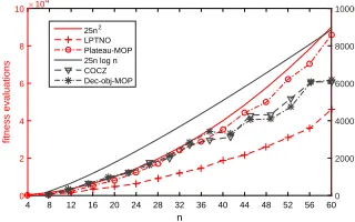
As shown in Figure 3, the curves of average fitness evalu-ations of numerical experiments (dash lines) on four prob-lems are approximately in the order of the corresponding theoretical bounds (solid lines), respectively. For ease of ob-servation, we plot curves of25n2and25nlognfor bounds
O(n2)andO(nlogn), respectively. This result confirms the
correctness of theoretical bounds obtained in our analysis.
n
4 8 12 16 20 24 28 32 36 40 44 48 52 56 60
fitness evaluations
×104
0 2 4 6 8 10
0 2000 4000 6000 8000 10000
25n2 LPTNO Plateau-MOP 25n log n COCZ Dec-obj-MOP
Figure 3: Curves of average fitness evaluations used in ex-periments, where MOEA/D-C runs 30 times for eachn.
Conclusions
In this paper, we present a theoretical analysis for the ef-fect of crossover in the MOEA/D framework. Our rigorous running time analysis shows that the MOEA/D-C working with several simple weight vectors can obtain a set of Pareto optimal solutions to cover the PF of four benchmark dis-crete optimization problems in expected running time better than the MOEA/D-M. This result suggests that the use of the crossover in the MOEA/D framework can simplify the complexity of the setting of the decomposed weight vectors and promote the efficiency of this kind of algorithms.
References
Chiang, T. C., and Lai, Y. P. 2011. MOEA/D-AMS: Improv-ing MOEA/D by an adaptive matImprov-ing selection mechanism.
InEvolutionary Computation, 1473–1480.
Dang, D. C.; Friedrich, T.; K¨otzing, T.; Krejca, M. S.; Lehre, P. K.; Oliveto, P. S.; Sudholt, D.; and Sutton, A. M. 2018. Escaping local optima using crossover with emergent di-versity. IEEE Transactions on Evolutionary Computation
22(3):484–497.
Doerr, B., and Doerr, C. 2018. Optimal static and self-adjusting parameter choices for the (1+(λ,λ)) genetic algo-rithm.Algorithmica80(5):1658–1709.
Doerr, B.; Johannsen, D.; K¨otzing, T.; Neumann, F.; and Theile, M. 2013. More effective crossover operators for the all-pairs shortest path problem. Theoretical Computer
Science471:12–26.
Doerr, B.; Doerr, C.; and Ebel, F. 2015. From black-box complexity to designing new genetic algorithms.
Theoreti-cal Computer Science567:87–104.
Giagkiozis, I.; Purshouse, R. C.; and Fleming, P. J. 2014. Generalized decomposition and cross entropy methods for many-objective optimization. Information Sciences
282:363–387.
Giel, O., and Lehre, P. K. 2010. On the effect of populations in evolutionary multi-objective optimisation*. Evolutionary
Computation18(3):335.
Ishibuchi, H., and Murata, T. 1998. A multi-objective genetic local search algorithm and its application to flow-shop scheduling. IEEE Transactions on Systems, Man, and
Cybernetics, Part C (Applications and Reviews)28(3):392–
403.
Ishibuchi, H.; Sakane, Y.; Tsukamoto, N.; and Nojima, Y. 2010. Simultaneous use of different scalarizing functions in MOEA/D. In Genetic and Evolutionary Computation Conference, GECCO 2010, Proceedings, Portland, Oregon,
Usa, July, 519–526.
Ishibuchi, H.; Setoguchi, Y.; Masuda, H.; and Nojima, Y. 2017. Performance of decomposition-based many-objective algorithms strongly depends on pareto front shapes. IEEE
Transactions on Evolutionary Computation21(2):169–190.
Jansen, T., and Wegener, I. 2002. On the analysis of evo-lutionary algorithms - a proof that crossover really can help.
Algorithmica34(1):47–66.
Jansen, T. 2013. Analyzing evolutionary algorithms: The
computer science perspective. Springer Science & Business
Media.
K¨otzing, T.; Sudholt, D.; and Theile, M. 2011. How crossover helps in pseudo-boolean optimization. In Pro-ceedings of the 13th annual conference on Genetic and
evo-lutionary computation, 989–996. ACM.
Laumanns, M.; Thiele, L.; Zitzler, E.; Welzl, E.; and Deb, K. 2002. Running time analysis of multi-objective evolutionary algorithms on a simple discrete optimization problem. In
International Conference on Parallel Problem Solving from
Nature, 44–53. Springer.
Laumanns, M.; Thiele, L.; and Zitzler, E. 2004. Running time analysis of multiobjective evolutionary algorithms on pseudo-boolean functions.IEEE Transactions on
Evolution-ary Computation8(2):170–182.
Lehre, P. K., and Yao, X. 2011. Crossover can be construc-tive when computing unique input–output sequences. Soft
Computing15(9):1675–1687.
Li, Y.-L.; Zhou, Y.-R.; Zhan, Z.-H.; and Zhang, J. 2016. A primary theoretical study on decomposition-based mul-tiobjective evolutionary algorithms. IEEE Transactions on
Evolutionary Computation20(4):563–576.
Li, K.; Kwong, S.; Zhang, Q.; and Deb, K. 2017. Interrelationship-based selection for decomposition multi-objective optimization. IEEE Transactions on Cybernetics
45(10):2076–2088.
Murata, T., and Gen, M. 2002. Cellular genetic algorithm for multi-objective optimization. In Proc. of the 4th Asian
Fuzzy System Symposium, 538–542. Citeseer.
Neumann, F., and Theile, M. 2010. How crossover speeds up evolutionary algorithms for the multi-criteria all-pairs-shortest-path problem. InInternational Conference on
Par-allel Problem Solving from Nature, 667–676. Springer.
Qi, Y.; Ma, X.; Liu, F.; Jiao, L.; Sun, J.; and Wu, J. 2014. MOEA/D with adaptive weight adjustment. Evolutionary
computation22(2):231–264.
Qian, C.; Yu, Y.; and Zhou, Z.-H. 2013. An analysis on recombination in multi-objective evolutionary optimization.
Artificial Intelligence204:99–119.
Sudholt, D. 2013. A new method for lower bounds on the running time of evolutionary algorithms.IEEE Transactions
on Evolutionary Computation17(3):418–435.
Sudholt, D. 2017. How crossover speeds up building-block assembly in genetic algorithms. Evolutionary Computation
25(2):237–274.
Tanabe, R., and Ishibuchi, H. 2018. An analysis of con-trol parameters of MOEA/D under two different optimiza-tion scenarios. Applied Soft Computing70:22–40.
Trivedi, A.; Srinivasan, D.; Sanyal, K.; and Ghosh, A. 2017. A survey of multiobjective evolutionary algorithms based on decomposition.IEEE Transactions on Evolutionary
Compu-tation21(3):440–462.
Wang, R.; Xiong, J.; Ishibuchi, H.; Wu, G.; and Zhang, T. 2017. On the effect of reference point in MOEA/D for multi-objective optimization. Applied Soft Computing58. Wang, R.; Zhang, Q.; and Zhang, T. 2016. Decomposition-based algorithms using pareto adaptive scalarizing
meth-ods. IEEE Transactions on Evolutionary Computation
20(6):821–837.
Zhang, Q., and Li, H. 2007. MOEA/D: A multiobjec-tive evolutionary algorithm based on decomposition. IEEE
Transactions on evolutionary computation11(6):712–731.
Zhou, A.; Qu, B.-Y.; Li, H.; Zhao, S.-Z.; Suganthan, P. N.; and Zhang, Q. 2011. Multiobjective evolutionary algo-rithms: A survey of the state of the art. Swarm and