The Evolution of Vagueness
Cailin O’Connor
January 23, 2013
1
Introduction
Vague predicates, those that exhibit borderline cases, pose a persistent problem for philosophers and logicians. Although they are ubiquitous in natural language, when used in a logical context, vague predicates lead to contradiction. This paper will address a question that is intimately related to this problem. Given their inherent imprecision, why do vague predicates arise in the first place?
Following the 1969 publication of David Lewis’ Convention, philosophers and game theorists have used signaling games to model the evolution and development of language.1 In this paper, I will present a variation of a standard signaling game
that can help inform how and why vague predicates develop. The model in question will consider signaling games where the states of the world are contiguous. What I mean by this is that states of the world may be ordered by similarity as they are in the sorts of situations in which vague predicates typically arise. A ‘heap’ with 1 million grains is very similar to one with 999,000 grains, quite similar to one with 800,000 grains, and increasingly less similar to smaller and smaller heaps. With a small alteration, the standard Lewis signaling game can be taken as a model of the development of signaling in such situations. I will also consider an alteration to Herrnstein reinforcement learning dynamics intended to better reflect the type of generalized learning real-world actors use when states of the world are contiguous. Under these alterations, actors in these models quickly and successfully develop signaling conventions where adjacent states are categorized under one signal, as they are in prototypically vague predicates.
Furthermore, the predicates developed in these simulations are vague in much the way ordinary language predicates are vague—they undoubtedly apply to cer-tain items, and clearly do not apply to others, but for some transition period
1See recent work by Jeffrey Barrett, Andreas Blume, Michael Franke, Simon Huttegger,
it is unclear whether or not the predicate applies. In other words, they exhibit borderline cases. These models may help explain why vagueness arises in natu-ral language: the real-world learning strategies that allow actors to quickly and effectively develop signaling conventions in contiguous state spaces make it un-avoidable. This ‘how-possibly’ story for the evolution of vagueness is particularly interesting given previous game theoretic results due to Lipman [2009] indicating that, generally, vagueness is inefficient in common-interest signaling situations. The implication is that, while vagueness itself may not be evolutionarily benefi-cial, it may nonetheless persist in language because learning strategies that are themselves evolutionarily beneficial lead to vagueness.
The paper will proceed as follows. In section 2, I will explain the workings of the standard signaling game and discuss a modification, first presented by J¨ager [2007], that better represents the development of signaling when states of the world are contiguous. For simplicity’s sake, I will call the games defined by this modification contiguous signaling (CS) games. In the following section, I will discuss some equilibrium properties of CS games. In section 4, I will present results obtained by evolving CS games using learning dynamics. The dynamics considered will include Herrnstein reinforcement learning and an alteration to this dynamic that I will call generalized reinforcement learning. As I will show, under this second learning dynamic, actors in CS games dependably develop signaling conventions that are both successful and persistently vague. In the last section, I will discuss the character of explanation these models provide, the ways in which vagueness is embodied in the models, and connections between this work and previous game theoretic work on vagueness.
2
Contiguous Signaling Games
The goal of this section is to present a game that appropriately models the devel-opment of signaling when states of the world are contiguous. The Lewis signaling game, commonly used to model information transfer and communication, is taken as the starting point.
temperature and signal to her father who will either bring coats or fans out of the garage. If the father brings the appropriate items, both receive a payoff (comfort). If he fails, no such payoff is acheived.2
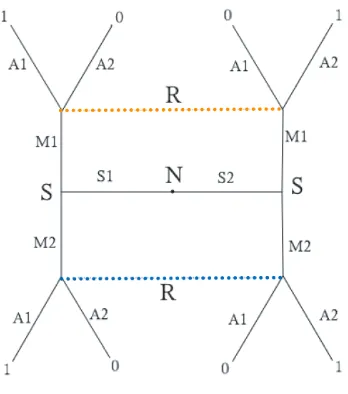
Figure 1 shows the extensive form of this game with two possible states of the world, two possible signals, two possible acts, and a payoff of 1 for coordination. The figure should be read as a decision tree beginning with the central node of the diagram. This node is labelled N, for ‘nature’, and represents the first move in the game wherein exogenous factors (nature) determine the state of the world to be S1, state 1, or S2, state 2. The two nodes labelled S represent the next move in the game where the sender observes one of these two states and either chooses M1, message 1, or M2, message 2. The final move involves the receiver, R, observing M1 or M2 and choosing A1, act 1, or A2, act 2. Dotted lines connect nodes on the graph that are indistinguishable for the receiver. The payoff for both players for each possible path is represented by the number at the end of it.
Figure 1: Extensive form game tree for a 2 state/act, 2 signal signaling game. The first decision node is labeled ‘N’ for nature. Payoffs are identical for both actors.
In applying the signaling game to the development of vague predicates, it is first necessary to consider the types of conditions under which vagueness typi-cally arises. Doing so will make clear what sorts of alterations to the traditional game will best represent these real-world situations. The first thing to note is that vague predicates typically arise when actors are attempting to convey information about a world with many possible states, i.e., a world with a large state-space.
For example, the prototyically vague predicate ‘bald’ is intended to transfer infor-mation about the number of hairs on a human head, which may range from 0 to approximately 100,000.
This suggests that one should investigate a signaling game with many potential states and acts. But unfortunately, prior work in evolutionary game theory has shown that this plan is doomed from the start. While in two state/act games, senders and receivers easily develop signaling conventions under a variety of evolu-tionary and learning dynamics, in larger games this success quickly breaks down. Under the replicator dynamics—the widest studied and most ubiquitous change algorithm employed in evolutionary game theory—it has been shown that Lewis signaling games with more than two states do not always evolve populations where actors ideally use signals to coordinate behavior.3 Learning dynamic results from
Barrett [2009] indicate that as the number of states in a signaling game gets larger, the likelihood of actors developing strategies that successfully coordinate behav-ior declines. For example, even in an 8 state/act game, actors failed to develop successful signaling strategies in almost 60 percent of simulations using reinforce-ment learning dynamics. So simply considering games with many states of nature clearly cannot provide information about the evolution of vague predicates. In fact, previous results seem to indicate that language should be unlikely to evolve at all in such large state spaces! Clearly something else is needed.
In most real-world situations where vagueness arises, however, the state space has additional structure: the states admit a natural ordering by similarity. In some cases of vagueness, the properties in question exist in a contiguous state space (bald, heap), while in others they exist in a state space that is actually con-tinuous (length, size, temperature, time duration). In both cases it is clear that there are similarity relations over the various possible states of the world—a 30 degree day is more like a 35 degree day than a 90 degree day.4 Of course, this
appeal to ‘similarity’, while intuitive, is not very precise. How should ‘similar-ity’ between states be interpreted here? Perhaps the best way of understanding these observations invokes measurement theory and psychology. Some phenom-enal experiences can be mapped to a space with a metric that represents their phenomenal similarity.5 For example, human color experience can be fairly
effec-3For more on this see Huttegger [2007], Huttegger et al. [2010], and Pawlowitsch [2008]. 4It might be taken as an objection to the models I present in this paper that they have only
discrete state spaces, and thus cannot represent properties that vary continuously. In similar work, both J¨ager [2007] and Komarova et al. [2007] appeal to the psychological notion of just-noticeable-differences in justifying the choice to treat continuous state spaces as discrete for modeling purposes. The choice here should best be understood as a simplifying assumption that allows for tractability while preserving the most important aspect of the state space in the models, its underlying similarity structure.
tively mapped to a spindle-shaped space whose axes represent hue, saturation, and brightness.6 One way to interpret the state spaces in the signaling games here is as representing these phenomenal spaces, rather than representing a space that maps physical, real-world objects. Under this interpretation, signaling about properties whose phenomenal character does not neatly correspond to real world character— paradigmatic examples include color and hardness—can still be modeled using these games.
Importantly, the fact that similarity relations hold over states of the world in the cases at hand means that an action taken by a receiver may vary in its level of success. Consider a sender who is drawing a mural and requests that the receiver pass her a blue crayon. If several of the available crayons are blue, the sender will be happy with any of them to one degree or another. The teal crayon may please her less well, though it will certainly be better received than the yellow one. In this way, the action taken by the receiver may be perfectly appropriate (just the blue the sender wanted), moderately appropriate (teal), or completely inappropriate (yellow). Given this observation, the payoff structure of a typical signaling game—either full payoff for perfect coordination, or no payoff for lack of coordination—does not appropriately capture the relevant aspects of real-world signaling situations where vague predicates arise. In these situations payoffs vary, because acts exhibit varying degrees of appropriateness for the state. In order to use signaling games to understand the evolution of vague predicates, a modification must be made to the payoff structure of these games.
The modification I will consider is one first proposed by J¨ager [2007]. The modified game works just as a normal signaling game, with one exception. The sender and receiver are, as before, most stongly rewarded when the act taken and state observed are perfectly matched, but they are also rewarded when the act and state are nearly matched. Payoffs are not binary, but rather vary according to the distance between the state of the world and the state for which the act taken was most appropriate.
In order to calculate the strength of reward given a certain state and act, the game incorporates a payoff function over the distance between them. Obviously this function should decrease in distance, as payoff should be lower when an act is less appropriate for a state. There are several functions that could work given the setting. In this paper I will primarily investigate games where payoffs are modeled by gaussian functions (otherwise known as normal distributions or ‘bell-curves’). Because these functions strictly decrease in distance, and always remain positive, they are particularly convenient from a modeling perspective. Although this choice may seem arbitrary from an interpretational standpoint, qualitative simulation results are robust under the choice of function, as are the analytic
results in many cases, as long as the most important aspect of the function is preserved, that it decrease in distance.
The game described has four parameters—the number of states/acts, the num-ber of signals, and two parameters determining the payoff function. In the case where payoff is determined by a gaussian function, these two parameters are the height and width. For those unfamiliar with these functions, the height refers to the highest point of the function above the x-axis and the width to how wide the function is at half the maximum height, i.e., how quickly it drops off as one moves away from the peak. Height, then, corresponds to the level of payoff that the actors in the game receive for perfect coordination, while width corresponds to how important it is that the players exactly coordinate behavior as opposed to approximately coordinating behavior. If the payoff gaussian is wide, players will recieve high payoffs for even imperfect coordination, while a narrow payoff gaussian will correspond to a situation where the act must nearly match the state to garner significant payoff. For simplicity sake, in the remainder of the paper, I will call the set of games just described contiguous signaling (CS) games.7 As will
become clear in the next sections, in which I present some analytic and simulation results, the modification in payoff structure in these games from that of standard games has a very dramatic effect on the development of signaling.
3
Equilibria
The goal of this section will be to analyze the equilibrium structures of CS games. This will be useful for two reasons. 1) The analysis will shed light on why the mod-els in the next section—where these games are evolved using learning dynamics— work the way the do. 2) It will also bring attention to a relevant feature of CS games: vagueness in these games is inefficient.
There are a few terms that will be useful in the following discussion. A Nash equilibrium for a game is a set of strategies from which no single player can deviate and improve her payoff. A pure strategy Nash equilibrium is one in which players do not play probabilistically. In other words, given a certain decision node in the game, a player’s action is fully determined. In a mixed strategy, on the other hand, players do not always perform the same actions, but rather mix over a number of strategies probabilistically. Payoff dominant, or efficient, Nash equilibria are those where players recieve the highest payoffs possible given the structure of the game. Before continuing, it will also be useful to discuss the types of equilibria seen in standard signaling games. David Lewis defined the term ‘signaling system’ to refer to strategies in signaling games where one signal is associated with each state,
7These games are actually a subset of those outlined by J¨ager [2007], whose model is much
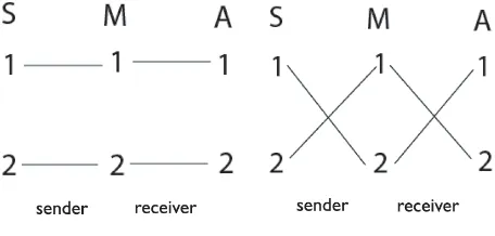
and where each signal induces the appropriate act for that state. In other words, where the actors perfectly coordinate behavior in every state of the world through the use of signals. Such strategies are often represented by a diagram like the ones shown in figure 2. Consider the diagram on the left first. In this diagram, S stands for state, M for message (again used instead of S for signal to disambiguate), and A for act. The numbers under S represent state 1 and state 2, etc. The left set of lines represent a pure sender strategy, which is a map from states of the world to signals, while the lines on the right represent a pure receiver strategy, a map from signals to acts. This particular diagram is of a 2 state/act, 2 signal game. The strategy represented is one where the sender chooses signal 1 in state 1 and signal 2 in state 2, and the receiver chooses act 1 given signal 1 and act 2 given signal 2. The diagram on the right represents the other signaling system possible in this game—where the actors perfectly coordinate, but using opposite signals.
Figure 2: The two signaling systems in 2 state/act, 2 signal, signaling games. These diagrams should be read as maps from states of the world (S), to signals (or messages, M), to acts (A). In this way they represent both sender and receiver strategies.
used to describe them. Later, I will restrict attention to games with fewer signals than states for this reason.
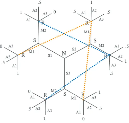
I will now consider some equilibrium properties of CS games. The simplest CS game of interest is a 3 state/act, 2 signal game. The extensive form of this game is shown in Figure 3, which should be read in the same way as Figure 1 with the obvious addition of S3 and A3 to represent state three and act three. The payoffs in this figure correspond to a linear function with slope of -.5 and a height of 1—perfect coordination receives a payoff of 1, a distance of one between state and act receives a payoff of .5, and a distance of two receives a payoff of 0.
Figure 3: 3 state/act, 2 signal game with modified payoffs.
A 3 state/act, 2 signal signaling game with a standard payoff structure (payoff for perfect coordination only) has 18 pure strategy Nash equilibria. The CS game with strictly decreasing payoffs8, on the other hand, has either 10 or 12 pure
strategy Nash equilibria, depending on how quickly the payoff function drops off. In the next simplest game of interest, the 4 state/act, 2 signal game, the reduction in pure strategy equilibria is even more dramatic. The standard game has 55 pure strategy Nash equilibria, but the CS game has either 16 or 24. In the 3 state/act,
8The results presented here are all for games where payoff is strictly decreasing in distance
3 signal game, the decrease in equilibria is also notable. The normal game has 87 pure strategy Nash equilibria, and the modified game has 57 or 63.
Why the reduction in pure strategy Nash equilibria given the change in payoff structure? This difference is primarily the result of a reduction of partial coordi-nation equilibria. This occurs because, given the payoff structure in CS games, strategies where 1) the sender assigns signals to nearly evenly sized, convex subsets of states and 2) the receiver, for any signal, takes an act that corresponds to the most central state associated with that signal, outperform other strategies. In fact, the payoff dominant equilibria in these games will always display these properties.9
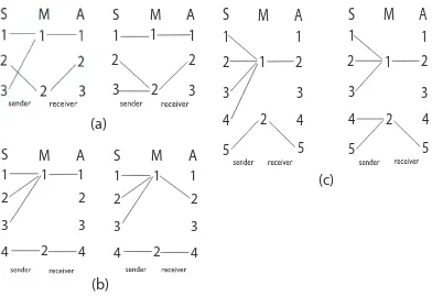
Figure 4 illustrates examples of the equilibrium strategies that are eliminated in CS games because they do not exhibit these properties. In each case, the strategies in both diagrams are equilibria of the standard signaling game, but the strategy on the left is not an equilibrium of the corresponding CS game. These diagrams should be read just like the diagrams in figure 2.
To see why these strategies are payoff dominant in CS games, consider that the best strategies in CS games will minimize the average distance between state and act thereby maximizing payoff. Given a sender strategy for any particular signal, the receiver can minimize average distance by playing the act that is appropriate for the median of the states associated with that signal. Given this type of best response on the part of the receiver, the sender then minimizes distance by using signals for only convex groups of states, and making those groups as small as possible, i.e., splitting the state space equally or nearly equally depending on the number of states.10 These facts about the payoff dominant Nash equilibria of CS games not only mean that the number of equilibria is reduced in these games, but that thebest equilibria are reduced whenever states outnumber signals. Furthermore, the larger the CS game, and the smaller the number of signals, the more significant the reduction in equilibria. This occurs because larger games have proportionately fewer equilibrium strategies where signal assignment is convex, etc. As will become clear in the next section, equilibrium selection in evolutionary models of these games seems to be eased by these reductions in equilibria.
Vague predicates are those with borderline cases. What, though, does a bor-derline case consist of in a CS game? In this paper I will consider as vague those strategies where the sender mixes signals, i.e., plays probabilistically, over some border between regions of signal application. In such strategies, signals apply cer-tainly in some states and not in others, but also have borderline regions of unclear application. In the next section examples of this phenomenon will be provided,
9Note that this assertion applies only to games where each state of the world arises with equal
probability, as is the case in all the games considered here. In games where some states are more likely to be selected by nature than others, the equilibrium results will be slightly different.
10J¨ager [2007] and J¨ager et al. [2011] have proven very similar results in a more general class
3
-
!
3
-
!
3
-
!
A
B
C
3
-
!
3
-
!
Figure 4: Three diagrams representing payoff dominant equilibrium strategies that are elimi-nated in CS games. In each case, both strategies are equilibria of the standard game, but only the strategy on the right is an equilibrium of the CS game. Diagram (a) shows a non-convex assignment of signals. Diagram (b) shows a strategy where the receiver does not take an ap-propriate act for the central state associated with a signal. Diagram (c) shows convex signal assignments, but that are not evenly sized.
but for now it should be noted that the payoff dominant equilibria of CS games do not exhibit vagueness as to signal meaning, as they are not mixed strategies.11
It is clear in these equilibria which states a term applies to and which it does not. The analysis here thus indicates that vagueness is inefficient in CS games. This observation echoes a proof by Lipman [2009] who showed that in common interest signaling situations, “vagueness [understood as a mixed strategy] cannot
have an advantage over specificity and, except in unusual cases, will be strictly worse” (4). This is significant for the following reason. In providing an evolu-tionary explanation of vagueness in signaling situations, it will be impossible to appeal to payoff benefits of vague strategies.12 Some other explanation will have
11There are knife’s edge cases where a low level of mixing can exist as part of a payoff dominant
Nash equilibrium of a CS game, but these are conceptually insignificant and will not be discussed here.
to be provided for the long-term persistence of vagueness in settings of common interest communication. In the next section, a possible explanation of this sort will be introduced.
4
Reinforcement Learning
In this section, I will present two sets of evolutionary models of the development of signaling in contiguous state spaces. In the first set of models, CS games will be evolved using a learning dynamic called Herrnstein reinforcement learning. In the second set of models, CS games will be evolved with a modification of Herrnstein reinforcement learning that I will call generalized reinforcement learning for the remainder of the paper. As will become clear, under both learning dynamics, the actors in these models develop signaling conventions that mirror those described in the previous section. However, the character of the signals developed under the two dynamics is different. Under Herrnstein reinforcement learning, the signals developed tend to have sharp boundaries, i.e., do not display significant signal vagueness. Under generalized reinforcement learning, however, the signals devel-oped are persistently vague. I will also explore the outcomes of these two sets of models in parameter space, and argue that there are parameter settings where the dynamics that lead to vagueness also lead to more successful signaling strategies, despite the inherent inefficiency of vagueness in these games.
There are many types of learning dynamics that can be applied to signaling games. Herrnstein reinforcement learning, first proposed by Roth and Erev [1995], is so named in reference to R. J. Herrnstein’s psychological work on learning which motivates the model. This learning dynamic has been widely used to study signal-ing games because 1) it is psychologically natural, i.e., based on observed learnsignal-ing behavior,13 and 2) it makes minimal assumptions about the cognitive abilities of
the actors. When complex signaling behaviors develop under models with this dynamic, then, a compelling how-possibly story for the development of the trait may be told, as even cognitively unsophisticated actors may exhibit the behavior in question. Herrnstein learning involves reinforcing the inclinations of the actors based on the past success of their strategies. This dyamic is often described as ‘urn learning’. Imagine that for each decision node in a game, a player has an urn
the interests of the sender and receiver are perfectly aligned. Standard signaling games represent such cases because the sender and receiver always garner the same payoff, and thus always prefer the same outcomes. There are signaling games, however, where the interests of the players are not aligned, and it has been shown by Blume and Board [this issue] and De Jaegher [2003] that in some of these cases vagueness may persist in equilibrium. However, real-world linguistic vagueness clearly includes cases where there is little or no conflict of interest between sender and receiver, so these models alone cannot explain the full phenomenon of vagueness.
filled with colored balls—one color for each action she might take at that decision node. Upon reaching a decision node, she reaches into the urn and chooses a ball randomly. The color of the ball determines which action she will take at that node. In a simulation, actors play a game many times. It is assumed that for the first round of play, each urn has exactly one ball of each color. In other words, chances that a player will choose any particular action are exactly even. If, however, the actors are successful in a round of play, they reinforce whatever actions led to that success by adding a ball (or more than one) of the appropriate color to the appropriate urn. Then in the next round of play, the chances of the actors taking a previously successful action are higher.14
A simulation of a CS game under this dynamic works just as a simulation of a standard game, but the inclinations of the sender and receiver are incremented even when the state-act match is imperfect. To give an example, suppose we consider a model with 10 states/acts, 2 potential signals, and payoffs modeled by a gaussian with a height of 5, and a width of 5. Suppose that in the first run of the simulation, nature determines the state to be 5. The sender observes this state and happens to choose the signal ‘1’ (although she might with equal likelihood have chosen ‘2’). The receiver observes the signal and happens to choose act ‘6’ (although she might have chosen any other act 1–10 with equal likelihood). The distance between state and act is 1, and so the payoff is determined according to the payoff function to be 4.61. The actors then reinforce the actions that were successful according to this payoff. The sender adds 4.61 signal 1 ‘balls’ to the state 5 urn. The receiver adds 4.61 act 6 balls to the signal 1 urn. In the next round, the sender chooses signal 1 in state 5 with a probability of .85 and signal 2 with .15. The receiver chooses act 6 given signal 1 with a probability of .38, and each other act with a probability of .068. In other words, in the next round the sender and receiver play strategies where they are more likely to repeat the actions that worked last time.
Under generalized reinforcement learning, the actors update their strategies from round to round of a simulation similarly to under Herrnstein learning, but with one key distinction. Under this new dynamic players reinforce over states and acts for successful coordination, but also reinforce (to a lesser degree) on
nearby states and acts. In other words, upon successful coordination senders and receivers will be more likely to repeat their successful behavior, but they will also be more likely to repeat similar behavior. The name of this dynamic is chosen for its relationship to the psychological phenomenon of stimulus generalization, which will be discussed more extensively in the next section. To give a quick example of the type of learning this dynamic models, suppose you are in a state of hunger
14For a good review of dynamics used to investigate signaling games, including learning
(I will call your hunger state ‘10’), you send me the signal ‘Reese’s Pieces’, and I give you a handful of 20 candies. What this dynamic supposes is that the next time you are in any hunger state near 10 you will be more likely to signal ‘Reese’s Pieces’, and the next time I receive that signal I will be more likely to give you a handful of any number near 20.
It is necessary, for this dynamic, to specify how many neighboring states and acts are reinforced, and how quickly the level of reinforcement drops off. As before, various functions might be appropriate and once again I have focused on gaussian functions for simplicity’s sake.15 It should be emphasized that the function in
question now does not determine thelevel of reinforcement for the state of nature and the act taken—that level is still determined as before, as a gaussian function of the distance between state and act. Rather, given the level of reinforcement for the actual state of nature and act performed, a second gaussian function determines the level of reinforcement over nearby states and acts.
To clarify how generalized reinforcement learning works, let us reconsider the last example, but now determining reinforcement levels using a gaussian function with a width of 2. (Note that this model adds one parameter value to the previous model—the width of the reinforcement function.) Nature chooses state 5 and the sender observes this state and sends signal 1. The receiver observes signal 1 and chooses act 6. The distance between the state and act is 1, so the sender adds 4.61 signal 1 balls to the state 5 urn. At the same time, though, the sender adds 2.79 balls to the state 4 and state 6 urns, and .62 balls to the states 3 and 7 urns, and so on according to the reinforcement distribution. In the next round, the sender is significantly more likely to use signal 1 than signal 2 in a number of states. She will send signal 1 in state 5 with a .85 probability, in states 6 and 8 with a .79 probability, in states 7 and 3 with a .62 probability, etc. The receiver’s inclination to take acts 5 and 7, and acts 4 and 8 are likewise incremented. From this point forward, for simplicity’s sake, I will call models of CS games that use Herrnstein reinforcement learning ‘CS models’ and those that use generalized reinforcement learning ‘Vague Signaling’ or ‘VS models’ (for the phenomenon of vagueness that arises in them). It should be noted that CS models are, in fact, a limiting case of VS models. As the width of the reinforcement function in a VS model goes to 0, the model approaches a CS model.
Note that in a simulation using either of these dynamics, the strategies taken by the actors at some stage in the simulation will always be mixed strategies, as opposed to pure ones. In fact, under these dynamics, strategies are always fully mixed, meaning that at every decision node there is some positive probability that the actor will take any particular action (there will always be at least one ball
15And again, other strictly decreasing (and even just decreasing) functions yield similar
of each color in an urn). What develops over the course of the simulation are simply the probability weights the actors assign to each action available to them as determined by previous success. Over time, the strategies of the actors may develop to approximate, or converge to, pure strategies as the same successful actions are repeatedly reinforced.
Simulations of VS and CS models develop signaling conventions under a wide range of parameter settings. In particular, signaling develops in these models even when the number of states and acts is large, presumably because the reduction in Nash equilibria discussed in section 3 eases equilibrium selection. In models with hundreds of states and acts, actors can develop successful signaling conventions, a perhaps surprising result given the failure rates of much smaller standard games. Of further interest is the qualitative result that in these models the actors do actually develop signaling conventions where the sender tends to group adjacent states under the same signal, and given that signal the receiver either takes an act appropriate for a central state, or mixes over a number of acts appropriate to states represented by the signal. These strategies mimic the payoff dominant Nash equilibria described in the last section. (I say ‘tends to’ and ‘mimic’ here because optimality does sometimes evolve in these models in the form of non-convex signals, synonyms, vagueness, etc.) This result is of interest as it indicates that even actors with very simple learning strategies can solve two simultaneous coordination problems while learning to signal—that of dividing a contiguous state space into categories (groups of states that are treated as one for signaling and acting purposes), and that of conventionally choosing signals to represent those categories.
Although they share many qualitative features, the strategies that develop in CS and VS models are not qualitatively identical. As noted, all strategies devel-oped in CS and VS models are fully mixed as an artifact of the learning dynamics used. The strategies that develop in VS models, however, show much more sig-nificant and persistent mixing. In other words, the strategies in VS models are significantly and persistently vague. To get a better sense of how the signaling strategies developed in CS and VS models qualitatively differ, consider figure 5. In each graph, states of the world are mapped on the x-axis. The y-axis repre-sents the probability with which the sender uses various signals in each possible state. Each signal is represented by a colored (dotted) line, the height of which corresponds to the probability that it is used in a particular state. Figure 5 shows the same game, a 20 state/act, 3 signal game with a payoff gaussian of width 6, evolved using Herrnstein reinforcement learning and two generalized reinforcement learning dynamics, one with a reinforcement gaussian of width 2, and one with a reinforcement gaussian of width 4.
5 10 15 20State 0.2
0.4 0.6 0.8 1.0
Sender Strategy
HaL
5 10 15 20 State 0.2
0.4 0.6 0.8 1.0
Sender Strategy
HbL
5 10 15 20 State 0.2
0.4 0.6 0.8 1.0
Sender Strategy
HcL
Figure 5: Sender strategies at the end of 1 million run trials of a CS game under three different learning dynamics. Graph (a) shows a CS model. Graph (b) is of a VS model with a reinforcement function of width 2. Graph (c) is of a VS model with a reinforcement function of width 4. The x-axis maps states of the world. The y-axis maps the probability with which the sender uses any one signal in a state. Each line represents a signal used by the sender.
probability represent areas of signal vagueness. As is evident in these simula-tions, the signals developed in the VS models display more significant regions of vagueness than those in the CS model. Moreover, the VS model with a wider reinforcement function displays signals with more vagueness than those of the VS model with a narrower function. In fact, the levels of vagueness in these models may be quantified by measuring the average level of mixing in the strategy used by the sender. This is done by comparing the probability with which the two most likely signals are sent in any particular state, and determining the vagueness level in that state as follows.
Vagueness level in state i = 1 - [(Probability of the most likely signal used in i) - (Probability of the second most likely signal used in i)]
Note that if two signals are equiprobable in a state, the vagueness level in that state will be 1 (as vague as possible). If one signal is used with nearly perfect probability, and the other signal is practically never used, the vagueness level is calculated to be near 0.16 The overall level of vagueness for a set of
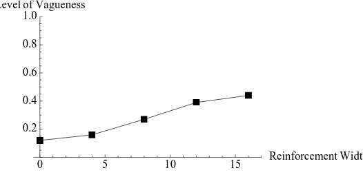
strategies in a simulation is then calculated by averaging the vagueness levels for each state. For the models shown in figure 5 (and one model with an even wider reinforcement function, of width 6) the levels of vagueness averaged over 50 trials of simulation are presented in figure 6. As is obvious in figure 6, the models with wider reinforcement gaussians are progressively more vague. This result occurs in games of other parameter values as well. In simulations of a 100 state/act, 5 signal game with payoff gaussian of width 10, the vagueness levels for different reinforcement functions were as shown in figure 7. These were also averaged over 50 trials of 1 million runs each. Once again, the wider reinforcement gaussians lead to strategies with higher levels of vagueness.
0 1 2 3 4 5 6 Reinforcement Width
0.2 0.4 0.6 0.8 1.0
Level of Vagueness
Figure 6: Average vagueness in simulations given different reinforcement functions. The x-axis maps various reinforcement function widths. The y-axis maps the level of vagueness developed.
0 5 10 15 Reinforcement Width
0.2 0.4 0.6 0.8 1.0
Level of Vagueness
Figure 7: Average vagueness in simulations given different reinforcement functions for a larger game.
It should be no surprise that VS models, especially those with wide reinforce-ment functions, display persistent vagueness as to signal meaning. To see why, imagine what happens at the boundary regions between signals in these models. If the sender and receiver successfully manage to coordinate behavior at a state in the boundary region, this behavior is reinforced. This means that the signal used is reinforced for that state, but also for nearby states, including ones further across the boundary region. Thus, in fact, the development of precise signaling will be impossible in these models. In CS models, on the other hand, precise signalingis
(essentially) possible. The distinction is best understood as follows. Because of the difference in learning dynamics in these models, the strategies in CS models may evolve to be abritrarily close to pure strategies, whereas the strategies in VS models may not.
As established in the last section, though, vagueness in CS games is inefficient. This means that the best strategies developed in VS models can never garner the payoff that the best strategies developed in CS models do. What the rest of this section will argue, however, is that under some parameter settings dynamics with wide reinforcement gaussians outperform those with narrow ones. In particular, I will explore how varying the length of a simulation, number of states, and number of signals influences the success of learning strategies and the development of vagueness in these models. As I will show, VS models with wider reinforcement functions are more successful in large state spaces with few signals when the actors have less time to develop strategies.
In discussions of standard signaling games and reinforcement learning, it is typ-ical to discuss how ‘successful’ the strategies developed by the actors are. Success, in these cases, refers to the expected payoff the actors receive divided by the ex-pected payoff received when playing a payoff dominant equilibrium. Expectation here refers to the average payoff earned over all the possible states nature might select. In a standard 4 state/act, 4 signal game with a payoff of 1 for coordination, for example, the players always receive a payoff of 1 if they play a signaling system. Then their expected payoff in a payoff dominant equilibrium is 1. If the actors play a strategy that allows for coordination in only three out of four states, the average payoff for this strategy is .75. Since the best average payoff possible is 1, the players have a success rate of 75 percent. The same measure will be used to determine how ‘successful’ the strategies developed by actors in the simulations here are. To be absolutely clear:
Success rate for a simulation = (Expected payoff given strategies of the actors)/(Expected payoff in a payoff dominant equilibrium)
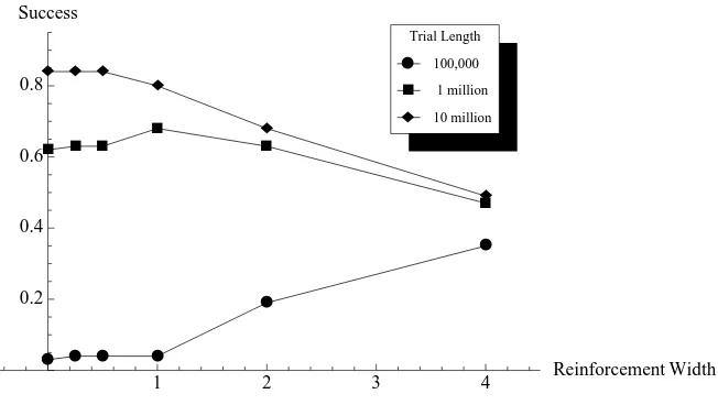
with wide reinforcement functions can outperform those with narrow functions. This is unsurprising—generalization allows actors to learn more quickly. As the length of a run increases, however, models with narrower reinforcement functions tend to outperform others because the strategies developed are less vague, and so garner better payoff. Figure 8 shows the various success rates in a 200 state/act, 40 signal game with a payoff function of width 4. Simulations of this game were performed for 100,000, 1 million, and 10 million runs and with reinforcement gaus-sian widths of 0 (a CS model), .25, .5, 1, 2, and 4. The success rates shown in this graph were averaged over 100 trials of these parameter settings. In the shortest trials pictured, those with 100,000 runs, the widest reinforcement width outper-forms the other models. In the mid-length trials, the reinforcement of width 1 is the most successful. And in the longest trials, the smaller reinforcement width allows for the greatest success.
æ æ æ æ
æ
æ à à à
à
à
à ì ì ì
ì
ì
ì
1 2 3 4 Reinforcement Width
0.2 0.4 0.6 0.8 Success
ì 10 million
à 1 million
æ 100,000 Trial Length
Figure 8: Success rates of CS and VS models by length of trial and width of reinforcement. The x-axis maps the width of the reinforcement function in the model. The y-axis maps the success of the strategies developed in the trial. Different markers represent different lengths of trial.
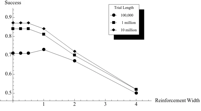
figure 9, narrow reinforcement functions outperform wider ones at much shorter trial lengths than in the otherwise identical 200 state game. This occurs because in larger games, the actors must learn to coordinate in more states. Strategies that allow swift coordination are then more effective. In smaller games, where coordination is more easily accomplished, more precise strategies do better, again, because they do not lead to signal vagueness.
æ æ æ æ
æ
æ à à à
à
à
à ì ì ì
ì
ì
ì
1 2 3 4 Reinforcement Width
0.5 0.6 0.7 0.8 0.9 Success
ì 10 million
à 1 million
æ 100,000 Trial Length
Figure 9: Success rates by length of trial and width of reinforcement for a smaller game. The x-axis maps the width of the reinforcement function in the model. The y-axis maps the success of the strategies developed in the trial. Different markers represent different lengths of trial.
æ æ æ æ
æ
æ à à à
à à
à ì
ì ì
ì ì ì
1 2 3 4 Reinforcement Width
0.5 0.6 0.7 0.8 0.9 Success
ì 10
à 20
æ 40 Signals
Figure 10: Success rates by number of signals and width of reinforcement for a 200 state game. The x-axis maps the width of the reinforcement function. The y-axis maps success rate of the model. Different markers represent different numbers of signals.
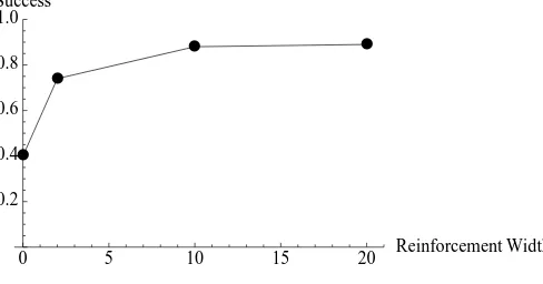
To give one more notable example of this phenomenon, consider a 1000 state/act game with 4 signals, and a payoff function of width 100. Figure 11 shows the suc-cess rates of models of this game with various reinforcement functions. These rates were averaged over 50 trials of 1 million runs each. In this case, wider does better. The model with a reinforcement gaussian of width 20 garners the highest success rate of those considered here. The success rate of this model is .89, while that of the CS model is .41.
æ æ
æ æ
0 5 10 15 20 Reinforcement Width
0.2 0.4 0.6 0.8 1.0 Success
Figure 11: Success rates by width of reinforcement for a 1000 state/act game.
vague predicates arise in situations where states of the world are numerous and the signals representing these states are few. At the very least, though, they support the conclusion that generalization, in the models presented here, is sometimes more effective than non-generalized learning despite the fact that this learning behavior leads to vagueness as to signal meaning. As will be discussed in the next section, this observation may help explain the evolution of vagueness.
5
Vagueness and VS models
The explanation of the evolution of vagueness presented here has two aspects. First, it is a how-possibly story about why persistent vagueness might arise in natural language at all. Lipman [2009], as mentioned, has shown that vagueness is suboptimal from a payoff standpoint in common-interest signaling situations. His work thus raises the question: if vagueness does not confer direct fitness benefits to signalers, why is it ubiquitous in natural language? An adequate explanation will have to appeal to something besides the direct benefits conferred by vague strategies to their users. A few such explanations have been offered,17 but the one
outlined here is novel.
The explanation of vagueness provided here is not just a how-possibly story, however. In VS models, the aspect of the model that leads to vagueness—the repetition of successful behavior in similar scenarios—is psychologically natural. Generalization, or stimulus generalization, is a learning behavior wherein an actor conditioned to one stimulus responds in the same way to other, similar stimuli. This type of learning is extremely well documented. For example Mednick and Freedman [1960], in a review article of stimulus generalization, discuss 127 studies on the phenomenon. These studies cover a wide variety of test subjects (from hu-mans to other mammals to birds) and a wide range of sensory stimuli. Since the 1960s, evidence for this phenomenon has only continued to accumulate. General-ized reinforcement learning differs from Herrnstein reinforcement learning precisely in that the actors generalize behavior, or apply learned behaviors to similar situa-tions, as real actors do in cases of stimulus generalization. Of course, generalized reinforcement learning does not fully (nor even approximately) capture the intrica-cies of human learning behavior. However, thefeature of generalized reinforcement learning that leads to vagueness closely corresponds to a documented feature of real-world learning behavior. This correspondence gives explanatory bite to the
17De Jaegher and van Rooij [2011] and van Rooij [2011] have argued that vagueness can
how-possibly story provided here.
There is a second aspect to the explanation of vagueness presented here which, in some ways, goes deeper than the first. I have made the argument that gen-eralization, when applied to signaling situations, leads to vagueness. But this explanation presents a further puzzle: why does learning generalization arise in signaling situations (and elsewhere for that matter) in the first place? In other words, a question still remains as to where the evolutionary benefit occurs that leads to linguistic vagueness. As work presented in the previous section indi-cates, under certain parameter values generalization in signaling situations leads to strategies that garner better payoffs than more precise learning does. In par-ticular, generalization allows for speed of learning, especially in large state spaces and when the number of signals available is limited. When these factors obtain, generalization may confer evolutionary benefits to learners that outweigh the pay-off costs of vagueness. Vagueness, then, could be explained as a side effect of an efficient learning strategy. Of course, this explanation is not fully supported by the work presented here. This paper only compares two learning dynamics. It might be argued that higher-rationality learning strategies exist that can satisfy both desiderata at once—allowing for swift development of signaling in large state spaces, without sacrificing the precision of the signals developed. An argument for the evolution of generalization as a way to learn more quickly will thus have to appeal to other considerations (the fact that it requires only minimal cogni-tion to employ, for example). Suffice it to say that the results regarding speed of learning with and without generalization hint at a promising deeper explanation of vagueness that bears further investigation.
There are a few complaints that might be lodged against VS models. Vagueness in these models is represented by mixed strategies. This follows Franke et al. [2011] who similarly model vagueness, and Lipman [2009] who argues that mixed strategies in signaling situations are the most obvious way for signals to be vague. However, there is room for dissatisfaction with this way of modeling vagueness. Many philosophers are committed to the idea that proper linguistic vagueness must involve higher-order vagueness.18 Higher-order vagueness requires not only
that terms exhibit borderline cases, but that the borderline cases exhibit borderline cases and so on. There must be uncertainty about which cases really are borderline, and which are clear cut. In VS models, on the other hand, for every state it is clear which signals are used, and to what degree. It is also clear where the borderline cases between signals begin and end. In other words, there is no uncertainty about the uncertainty. Thus, it might be argued, they do not account for an important aspect of the phenomenon. Even those who believe that higher-order vagueness is necessary for full, linguistic vagueness, though, may take VS models to
be at least partially explanatory of the phenomenon of vagueness. And those who do not believe that higher-order vagueness is a necessary part of vague language may be satisfied that the simulations here really do capture a phenomenon that appropriately models vagueness.
A further complaint that might be lodged agains VS models regards the de-gree to which vagueness is ‘built in’ to the model. As I have pointed out, the learning dynamics in these models lead inevitably to signal vagueness. Then, it might be argued, the result that vagueness arises is uninteresting. What should be recognized, however, is that the results of every mathematical model are ‘built in’ to some degree, otherwise they would not be the results of the model! This is only problematic when models have been reverse engineered to produce a desired result through the inclusion of irrelevant or unnatural features. As argued, this is not the case here. The aspect of the learning dynamics that leads to vagueness is psychologically natural. Furthermore, although the result may be inevitable, it is not prima facie obvious that generalized learning leads to signal vagueness. The models thus have explanatory merit for elucidating a previously unrecognized pattern.
The explanation for the evolution of vagueness provided here is not the only one of merit. Of particular interest is a model presented by Franke et al. [2011]. These authors argue that bounded rationality, i.e., imperfect choice behavior on the part of actors, can lead to the same sorts of vagueness modeled here (persistent mixing of strategies) in equilibrium. What their model supposes is that individual choice is stochastic; that, as they say, “people are often not only indecisive, but even inconsistent in that they make different choices under seemingly identical conditions, contrary to the predictions of classical rational choice theory” (11). It seems very likely that these authors are correct in that the cognitive limitations of actors are at least partially explanatory of linguistic vagueness. When states of the world are contiguous (or even continuous), as in the situations where vagueness arises, it may be difficult to differentiate highly similar states, which may lead to probabilistic choice behavior like that modeled by Franke et al. Furthermore, when states of the world are numerous, it may be cognitively costly to keep track of which signaling behavior is the correct one for each state. In these cases, behavioral strategies that are less cognitively demanding may be worth employing, even if they are less accurate.
References
J. A. Barrett. The evolution of coding in signaling games. Theory and Decision, 67:223–237, 2009.
A. Blume and O. Board. Intentional vagueness. Erkenntnis, this issue.
K. De Jaegher. A game-theoretic rationale for vagueness. Linguistics and Philos-ophy, 26:637–659, 2003.
K. De Jaegher and R. van Rooij. Strategic vagueness, and appropriate contexts. In A. Benz, C. Ebert, G. Jager, and R. van Rooij, editors, Language, Games, and Evolution, pages 30–59. Springer-Verlag, Berlin, Heidelberg, 2011.
M. Franke, G. J¨ager, and R. van Rooij. Vagueness, signaling and bounded ratio-nality. pages 45–59. Springer, 2011.
R. Herrnstein. On the law of effect. Journal of the Experimental Analysis of Behavior, 13(2):243–266, 1970.
S. M. Huttegger. Evolution and the explanation of meaning.Philosophy of Science, 74:1–27, 2007.
S. M. Huttegger and K. J. S. Zollman. Language, Games, and Evolution, chap-ter Signaling Games: Dynamics of Evolution and Learning, pages 160–176. Springer-Verlag, Berlin Heidelberg, 2011.
S. M. Huttegger, B. Skyrms, R. Smead, and K. J. S. Zollman. Evolutionary dy-namics of lewis signaling games: signaling systems vs. partial pooling. Synthese, 172:177–191, 2010.
G. J¨ager. The evolution of convex categories. Linguistics and Philosophy, 30: 551–564, 2007.
G. J¨ager, L. P. Metzger, and F. Riedel. Voronoi languages: Equilibria in cheap-talk games with high-dimensional types and few signals. Games and Economic Behavior, 73(2):517–537, November 2011.
N. L. Komarova, K. A. Jameson, and L. Narens. Evolutionary models of color categorization based on discrimination. Journal of Mathematical Psychology, 51 (6):359–382, 2007.
D. K. Lewis. Convention. Harvard University Press, Cambridge, MA, 1969.
B. Lipman. Why is language vague? 2009.
S. A. Mednick and J. L. Freedman. Stimulus generalization.Psychological Bulletin, 57(3):169–200, May 1960.
C. Pawlowitsch. Why evolution does not always lead to an optimal signaling system. Games and Economic Behavior, 63:203–226, 2008.
A. E. Roth and I. Erev. Learning in extensive-form games: Experimental data
and simple dynamic models in the intermediate term. Games and Economic
Behavior, 8:164–212, 1995.
B. Skyrms. Signals: Evolution, Learning, and Information. Oxford University Press, 2010.
K. van Deemter. Utility and language generation: The case of vagueness. Journal of Philosophical Logic, 38(6):607–632, 2009.
K. van Deemter. Not Exactly: In Praise of Vagueness. Oxford University Press, Oxford, 2010.
R. van Rooij. Vagueness and linguistics. In G. Ronzitti, editor, Vagueness: A Guide. Springer, Dordrecht, 2011.