Adv. Radio Sci., 12, 13–19, 2014 www.adv-radio-sci.net/12/13/2014/ doi:10.5194/ars-12-13-2014
© Author(s) 2014. CC Attribution 3.0 License.
A mixed finite-element formulation for the modal analysis of
electromagnetic waveguides featuring improved low-frequency
resolution of transmission line modes
R. Baltes1, J. Al Ahmar2, O. Farle1, and R. Dyczij-Edlinger1
1Chair of Electromagnetic Theory, Dept. of Physics and Mechatronics, Saarland University, Saarbrücken, Germany 2Chair of Microintegration and Reliability, Dept. of Physics and Mechatronics, Saarland University, Saarbrücken, Germany Correspondence to: R. Baltes ([email protected])
Received: 25 January 2014 – Revised: 12 May 2014 – Accepted: 6 June 2014 – Published: 10 November 2014
Abstract. This paper presents an improved finite-element formulation for axially uniform electromagnetic waveguides. It allows for both dielectric and conduction losses and covers the entire range from optics down to the static limit. Prop-agation coefficients of small magnitude, particularly those of transmission line modes in the low-frequency regime, are computed much more accurately than with previous ap-proaches.
1 Introduction
Since electromagnetic waveguides constitute generalized transmission line systems, they are of fundamental impor-tance for the design of electromagnetic devices. Because of complex geometries and inhomogeneous materials, analyt-ical solutions for the modal field patterns and propagation coefficients are often difficult to obtain or even unavailable. Numerical field simulation methods provide a powerful rem-edy. In particular the finite-element (FE) method stands out for its high convergence rates and great flexibility in model-ing geometry and materials.
Early approaches suffered from the occurrence of spuri-ous modes, but with the advent of H(curl)conforming ba-sis functions these problems were overcome. A great variety of FE formulations have been proposed: Some are in terms of the electric (Lee et al., 1991) or magnetic field intensity (Valor and Zapata, 1995), while others employ a magnetic vector potential and a electric scalar potential (Bardi and Biro, 1991; Polstyanko and Lee, 1995). They all provide ac-curate results for high frequencies, but very few can handle
the low-frequency (LF) (Vardapetyan and Demkowicz, 2003) or even the static case (Lee et al., 2003; Farle et al., 2004). Moreover, they incorporate electric conductivityσby means of an equivalent imaginary partε00of the electric permittivity (Lee, 1994), which breaks down when the angular frequency ωtends to zero, due to
ε00=σ
ω. (1)
All methods above lead to generalized algebraic eigenvalue problems for the square of the propagation coefficient. As will be detailed in Sect. 4.2, this strongly amplifies numeri-cal round-off error in propagation coefficients of small mag-nitude, e.g. waveguide modes close to cut-off and, more im-portantly, transmission line (TEM or quasi-TEM) modes in the LF regime.
To overcome these limitations, we propose in Sect. 2 the prototype of a mixed-field formulation in terms of the elec-tric field intensity E and the magnetic flux densityB. Its distinguishing feature is that the sought eigenvalue is the propagation coefficient itself rather than its square. The sug-gested approach incorporates conduction losses quite natu-rally and minimizes round-off errors in propagation coeffi-cients of small magnitude. In Sect. 3 we establish stability in the LF regime, by imposing suitable constraints.
14 R. Baltes et al.: Mixed finite-element formulation for electromagnetic waveguides
2 Formulation
We consider an axially uniform waveguidepointing in the ˆ
z direction. Its boundary0, with unit outward normal vec-tornˆ, is assumed to consist of perfect electric walls0E and perfect magnetic walls0H. Letbe connected and0E non-empty. We denote the wavenumber, speed of light, and char-acteristic impedance, respectively, of free space by k0,c0, andη0. The relative magnetic permeability µr, the relative electric permittivity εr, and the electric conductivityσ are assumed to be scalar-valued. Thanks to uniformity along the waveguide axis, the modal fields are given by waves propa-gating in±ˆzdirection. For the negativezˆdirection, we have the decomposition (Pozar, 2005, p. 93)
E= Et+Ezzˆexp(γ z), (2) B= Bt+Bzzˆexp(γ z), (3) where subscriptst andzdenote transversal and longitudinal components, respectively, and γ is the propagation coeffi-cient. Thus the differential operators∂zand∇simplify to
∂z=γ , (4)
∇ = ∇t+∂zzˆ= ∇t+γzˆ. (5) By applying Eqs. (2)–(5) to Faraday’s law and Ampere’s law,
∇ ×E= −jk0c0B, (6)
∇ ×µ−1r c0B=(jk0εr+σ η0)E, (7) we arrive at a homogeneous boundary value problem, given by the set of partial differential equations
ˆ
z×(γEt− ∇tEz)= −jk0c0Bt, (8) ˆ
z·(∇t×Et)= −jk0c0Bz, (9) ˆ
z×
γ µ−1r c0Bt− ∇tµ−1r c0Bz
=(jk0εr+σ η0)Et, (10) ˆ
z·(∇t×µ−1r c0Bt)=(jk0εr+σ η0) Ez, (11) subject to the boundary conditions
Ez =0 ˆ
n×Et =0 ˆ
n·Bt =0
on0E, (12)
µ−1r Bz =0 ˆ
n×µ−1r Bt =0 ˆ
n·εrEt =0
on0H. (13)
2.1 Finite-element representation
LetH1,Hcurl,Hdiv, andH0denote the Sobolev spaces with respect to the operator in superscript (Boffi et al., 2013, pp. 4). We define the subspaces
H1E:=nλ∈H1()|λ=0 on0E o
, (14)
Hcurl E :=
n
u∈Hcurl()| ˆn×u=0 on0 E
o
, (15)
Hdiv E :=
n
u∈Hdiv()| ˆn·u=0 on0 E
o
, (16)
and denote the corresponding finite-element spaces byV1 E⊂
H1 E,V
curl
E ⊂H
curl E ,V
div
E ⊂H
div E , andV
0⊂H0. The transver-sal and axial fields Et, Ez,Bt, Bz are discretized by ba-sis functions of lowest order (Zhu and Cangellaris, 2006, pp. 19), for their respective function spaces. LetNN denote the number of free nodes,NEthe number of free edges, and NF the number of faces in the mesh. Then
Ez= NN
X
k=1
xEz,kλk withλk∈VE1, (17)
Et= NE
X
k=1
xEt,kwk withwk∈VEcurl, (18)
c0Bz= NF
X
k=1
xBz,kWk withWk∈V0, (19)
c0Bt= NE
X
k=1
xBt,kvk withvk∈VEdiv. (20)
Note that Eqs. (19) and (20) have been scaled byc0, for nu-merical stability. The FE representations of the differential operators grad, curl, and div are given by the incidence matri-ces G∈RNE×NN, R∈RNF×NE, and D∈RNF×NE. Also, in
two dimensions, we have (Zhu and Cangellaris, 2006, pp. 26)
D=R. (21)
Since Eqs. (8) and (9) are in terms of fields represented on the primal mesh, they are discretized in strong form. In con-trast, Eqs. (10) and (11) are based on the fieldsH =µ−1B,
D=εE, andJ=σE. These reside on the dual complex and are thus considered in weak form. The resulting generalized algebraic eigenvalue problem reads
(A+jk0C)x= −γBx. (22) At this point it can be seen that the eigenvalue is the propa-gation coefficientγ itself rather than its square. The vector and the matrices in Eq. (22) are given by
x=
xBt xBz xEt xEz
, A=
0 0 0 −G
0 0 −R 0
0 −RTTBz −Tσt 0
GTT
Bt 0 0 Tσ z
,
B=
0 0 I 0
0 0 0 0
−TBt 0 0 0
0 0 0 0
, C=
I 0 0 0
0 I 0 0
0 0 −TEt 0
0 0 0 TEz
,
R. Baltes et al.: Mixed finite-element formulation for electromagnetic waveguides 15
where I denotes the identity matrix. The other submatrices are defined as
TBt,ij= Z
vi·µ−1r vjd withvi,vj ∈VEdiv, (24)
TBz,ij= Z
Wiµ−1r Wjd withWi, Wj ∈V0, (25)
TEt,ij= Z
wi·εrwjd withwi,wj ∈VEcurl, (26)
TEz,ij= Z
λiεrλjd withλi, λj∈VE1, (27)
Tσ z,ij=η0 Z
λiσ λjd withλi, λj∈VE1, (28)
Tσ t,ij=η0 Z
wi·σwjd withwi,wj ∈VEcurl. (29)
In absence of magnetic (dielectric) losses, we haveµr ∈R+ (εr ∈R+) everywhere, and the corresponding matrices TBt and TBz(TEtand TEz) are positive definite. In contrast, Tσ t and Tσ z are positive semi-definite, because σ >0 holds in the conductive region only.
3 Low-frequency behavior
Fork0=0, the eigenvalue problem of Eq. (22) reduces to
Ax= −γBx. (30)
The matrix A+γB turns out to be singular, for any value ofγ. We will analyze this effect and propose a suitable reg-ularization.
3.1 Analysis of instability
We decompose the waveguide cross-sectioninto the loss-less region ll, withσ =0, the lossy subdomainl, with σ >0, and their common interface00:
=l∪ll∪00. (31)
In view of Eq. (23), the eigenvalue problem for the static case, Eq. (30), is equivalent to
γxEt=GxEz, (32)
−RxEt=0, (33)
γTBtxBt+Tσ txEt= −RTTBzxBz, (34)
GTTBtxBt+Tσ zxEz=0. (35)
Consider the vectors
xEt,γ
xEz,γ
=
G γI
xN, (36)
x Bt,γ
xBz,γ
=
−T−1BtRTTBz γI
xF, (37)
withxF ∈RNF arbitrary and anyxN∈RNN satisfying
xN,i= (
0 if nodei∈l∪00, arbitrary if nodei∈ll.
(38)
Plugging Eqs. (36) and (37) into Eqs. (32)–(35) shows that these are satisfied for any arbitrary value ofγ. The vectors
uγ=
xBt,γ
xBz,γ
xEt,γ
xEz,γ
(39)
form the eigenspace corresponding to γ. To regularize the eigenvalue problem and eliminate the non-physical eigenvec-tors, we first analyze the vectorsuγ. LetEγ andBγ denote the fields represented by Eqs. (36) and (37), respectively. In view of Eq. (38),Eγ is nonzero in the lossless region only and, by Eq. (4), it is a gradient field. Similarly, it can be shown that the magnetic field strengthH corresponding to
Bγis a gradient, represented on the dual mesh. PluggingEγ andBγinto Eqs. (6) and (7) and taking the divergence yields
−jk0c0∇ ·Bγ =0, (40)
jk0c−10 ∇ ·εrEγ =0. (41)
It can be seen that, for k0=0, these fields are no longer forced to be source-free.
3.2 Stabilization
To stabilize the method, we impose the conditions
∇ ·B=0 in, (42)
∇ ·(ε0εrE)=0 inll, (43) similarly to (Polstyanko et al., 1997; Hiptmair et al., 2008), by introducing Lagrange multiplierspF andpN. The dis-crete representations of Eqs. (42) and (43) read
DxBt+γxBz=RxBt+γxBz=0, (44) ˜
INGTTEtxEt−γ˜INTEzxEz=0, (45) where the matrix˜IN selects the nodes belonging to the loss-less regionsll.
16 R. Baltes et al.: Mixed finite-element formulation for electromagnetic waveguides 4 R.Baltes et al.: Mixed Finite-Element Formulation for Electromagnetic Waveguides
stant magnetic field strengthH pointing inˆz direction. To
220
exclude the eigenpair(γ= 0,x=uc), we impose the orthog-onality constraint
xTcxBz= 0, (49) by introducing a Lagrange multiplierpc. Thus, the stabilized eigenvalue problem for the caseΓH=∅becomes
225
(Aˆ+jk0Cˆ)xˆ=−γBˆx, (50)
with ˆ A=
0 0 0 −G 0 RT 0 0 0 −R 0 0 0 xc
0 −RTT
Bz −Tσt 0 TEtG˜I T N 0 0
GTTBt 0 0 Tσz 0 0 0
0 0 ˜INGTTEt 0 0 0 0
R 0 0 0 0 0 0
0 xTc 0 0 0 0 0
, B=
0 0 I 0 0 0 0 0 0 0 0 0 I 0
−TBt0 0 0 0 0 0
0 0 0 0 −TEz˜ITN 0 0
0 0 0−˜INTEz 0 0 0
0 I 0 0 0 0 0 0 0 0 0 0 00
, 230 ˆ C=
I 0 0 0 0 0 0 0 I 0 0 0 0 0 0 0−TEt 0 0 0 0
0 0 0 TEz0 0 0
0 0 0 0 0 0 0 0 0 0 0 0 0 0 0 0 0 0 0 00
, xˆ=
xBt xBz xEt pN pF pc . (51)
All eigenvectors of (50) that exhibit non-vanishing La-grange multipliers, i.e. non-zero pN,pF or pc, are known to span a subspace without physical meaning. This means
235
the relevant subvectors do not solve the original eigenvalue problem (22). Rather than to purge such unwanted eigenvec-tors from the results, the authors prefer to shift the associated eigenvalues to infinity, so that they do not pollute the spec-trum. This is easily accomplished, by setting the columns of
240
Bthat belong to Lagrange multipliers to zero. The modified matrixBˆ reads
ˆ B=
0 0 I 0 0 0 0 0 0 0 0 0 0 0
−TBt0 0 0 0 0 0
0 0 0 0 0 0 0 0 0 0−˜INTEz0 0 0
0 I 0 0 0 0 0 0 0 0 0 0 0 0
, (52)
and the final form of the eigenvalue problem is given by
(Aˆ+jk0Cˆ)xˆ=−γBˆˆx. (53)
245
10−10 10−5 100 105 1010 0 50 100 150 200 250 300
Frequency in Hz
Re {
γ
} in 1/m
TE 10EB TE 10AV TE 10Ana TE20EB TE20AV TE20Ana
(a) Attenuation coefficient.
10−10 10−5 100 105 1010 0 50 100 150 200 250 300 350 400
Frequency in Hz
Im {
γ
} in rad/m
TE10EB TE10AV TE 10Ana TE 20EB TE 20AV TE 20Ana
(b) Phase coefficient.
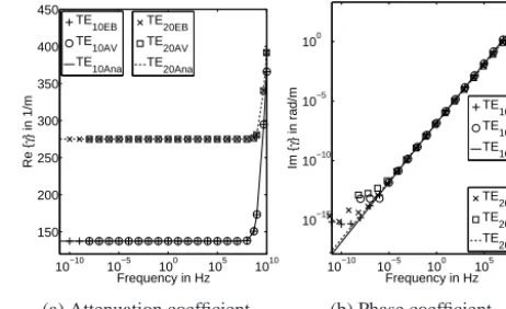
Fig. 1: Lossless rectangular waveguide: propagation coeffi-cients of TE10and TE20modes versus frequency.
10−10 10−5 100 105 1010 150 200 250 300 350 400 450
Frequency in Hz
Re {
γ
} in 1/m
TE 10EB TE 10AV TE 10Ana TE 20EB TE 20AV TE 20Ana
(a) Attenuation coefficient.
10−10 10−5 100 105 1010 10−15
10−10 10−5 100
Frequency in Hz
Im {
γ
} in rad/m
TE10EB TE10AV TE10Ana TE20EB TE20AV TE 20Ana
(b) Phase coefficient.
Fig. 2: Lossy RWG withσ= 5S/m: propagation coefficients of TE10and TE20modes versus frequency.
4 Numerical Examples
4.1 Rectangular Waveguide
We consider a rectangular waveguide (RWG) of dimensions
22.86mm×11.43mm with perfectly conducting walls and homogenous material properties (ǫr= 4,µr= 1) in both the
250
lossless case (σ= 0) and in presence of Ohmic losses (σ= 5 S/m). Our main goal is to demonstrate the correct function of the present approach and compare it to theA-V potential formulation of (Farle et al., 2004), a state-of-the-art method that solves forγ2and models conductivity via complex
per-255
mittivity (1). According to (Pozar, 2005, p. 108), the analyt-ical solution for the propagation coefficientγmnis given by
γmn=
r
mπ
a
2
+nπ b
2
−εrµrk02+jµrσk0η0, (54)
where a and b denote the width and height of the
wave-260
guide, respectively. Figs. 1 and 2 present the dispersion curves of the TE10and TE20modes in the frequency range
Figure 1. Lossless rectangular waveguide: propagation coefficients
of TE10and TE20modes versus frequency.
where Jiis the Jacobian matrix of facei. In view of Eq. (23), the corresponding kernel vector ofAreads
uc=
0 T−1Bzxc
0 0 . (47)
It is easy to verify that the fields ofucsatisfy Eqs. (32)–(35) and (45). Moreover, Eq. (44) implies
γ (uc)=0. (48)
Thus there exists a zero eigenvalue corresponding to a con-stant magnetic field strengthHpointing inzˆdirection. To ex-clude the eigenpair(γ=0,x=uc), we impose the orthogo-nality constraint
xTcxBz=0, (49)
by introducing a Lagrange multiplierpc. Thus, the stabilized eigenvalue problem for the case0H= ∅becomes
(Aˆ+jk0Cˆ)xˆ= −γBxˆ, (50) with ˆ A=
0 0 0 −G 0 RT 0
0 0 −R 0 0 0 xc
0 −RTTBz −Tσt 0 TEtG˜I
T
N 0 0
GTTBt 0 0 Tσ z 0 0 0
0 0 ˜INGTTEt 0 0 0 0
R 0 0 0 0 0 0
0 xTc 0 0 0 0 0
, B=
0 0 I 0 0 0 0
0 0 0 0 0 I 0
−TBt 0 0 0 0 0 0
0 0 0 0 −TEzI˜TN 0 0
0 0 0 −˜INTEz 0 0 0
0 I 0 0 0 0 0
0 0 0 0 0 0 0
,
4 R.Baltes et al.: Mixed Finite-Element Formulation for Electromagnetic Waveguides
stant magnetic field strength Hpointing in ˆz direction. To
220
exclude the eigenpair(γ= 0,x=uc), we impose the orthog-onality constraint
xTcxBz= 0, (49) by introducing a Lagrange multiplierpc. Thus, the stabilized eigenvalue problem for the caseΓH=∅becomes
225
(Aˆ+jk0Cˆ)ˆx=−γBˆx, (50)
with ˆ A=
0 0 0 −G 0 RT 0
0 0 −R 0 0 0 xc
0 −RTTBz −Tσt 0 TEtG˜I T N 0 0
GTT
Bt 0 0 Tσz 0 0 0
0 0 ˜INGTTEt 0 0 0 0
R 0 0 0 0 0 0
0 xT
c 0 0 0 0 0
, B=
0 0 I 0 0 0 0 0 0 0 0 0 I 0
−TBt0 0 0 0 0 0
0 0 0 0 −TEz˜ITN 0 0
0 0 0−˜INTEz 0 0 0
0 I 0 0 0 0 0 0 0 0 0 0 00
, 230 ˆ C=
I 0 0 0 0 0 0 0 I 0 0 0 0 0 0 0−TEt 0 0 0 0
0 0 0 TEz0 0 0
0 0 0 0 0 0 0 0 0 0 0 0 0 0 0 0 0 0 0 00
, xˆ=
xBt xBz xEt pN pF pc . (51)
All eigenvectors of (50) that exhibit non-vanishing La-grange multipliers, i.e. non-zero pN,pF or pc, are known to span a subspace without physical meaning. This means
235
the relevant subvectors do not solve the original eigenvalue problem (22). Rather than to purge such unwanted eigenvec-tors from the results, the authors prefer to shift the associated eigenvalues to infinity, so that they do not pollute the spec-trum. This is easily accomplished, by setting the columns of
240
Bthat belong to Lagrange multipliers to zero. The modified matrixBˆreads
ˆ B=
0 0 I 0 0 0 0 0 0 0 0 0 0 0
−TBt0 0 0 0 0 0
0 0 0 0 0 0 0 0 0 0−˜INTEz0 0 0
0 I 0 0 0 0 0 0 0 0 0 0 0 0
, (52)
and the final form of the eigenvalue problem is given by
(Aˆ+jk0Cˆ)ˆx=−γBˆˆx. (53)
245
10−10 10−5 100 105 1010 0 50 100 150 200 250 300
Frequency in Hz
Re {
γ
} in 1/m
TE 10EB TE 10AV TE 10Ana TE20EB TE20AV TE20Ana
(a) Attenuation coefficient.
10−10 10−5 100 105 1010 0 50 100 150 200 250 300 350 400
Frequency in Hz
Im {
γ
} in rad/m
TE10EB TE10AV TE10Ana TE20EB TE20AV TE20Ana
(b) Phase coefficient.
Fig. 1: Lossless rectangular waveguide: propagation coeffi-cients of TE10and TE20modes versus frequency.
10−10 10−5 100 105 1010 150 200 250 300 350 400 450
Frequency in Hz
Re {
γ
} in 1/m
TE10EB TE10AV TE10Ana TE20EB TE20AV TE20Ana
(a) Attenuation coefficient.
10−10 10−5 100 105 1010 10−15
10−10 10−5 100
Frequency in Hz
Im {
γ
} in rad/m
TE10EB TE10AV TE10Ana TE20EB TE20AV TE20Ana
(b) Phase coefficient.
Fig. 2: Lossy RWG withσ= 5S/m: propagation coefficients of TE10and TE20modes versus frequency.
4 Numerical Examples
4.1 Rectangular Waveguide
We consider a rectangular waveguide (RWG) of dimensions
22.86mm×11.43mm with perfectly conducting walls and homogenous material properties (ǫr = 4,µr = 1) in both the
250
lossless case (σ= 0) and in presence of Ohmic losses (σ= 5 S/m). Our main goal is to demonstrate the correct function of the present approach and compare it to theA-V potential formulation of (Farle et al., 2004), a state-of-the-art method that solves forγ2
and models conductivity via complex
per-255
mittivity (1). According to (Pozar, 2005, p. 108), the analyt-ical solution for the propagation coefficientγmnis given by
γmn=
r
mπ
a
2
+nπ b
2
−εrµrk02+jµrσk0η0, (54)
where a and b denote the width and height of the
wave-260
guide, respectively. Figs. 1 and 2 present the dispersion curves of the TE10and TE20modes in the frequency range
Figure 2. Lossy RWG withσ = 5 S/m: propagation coefficients of
TE10and TE20modes versus frequency.
ˆ C=
I 0 0 0 0 0 0
0 I 0 0 0 0 0
0 0 −TEt 0 0 0 0
0 0 0 TEz 0 0 0
0 0 0 0 0 0 0
0 0 0 0 0 0 0
0 0 0 0 0 0 0
, xˆ= xBt xBz xEt xEz pN pF pc . (51) All eigenvectors of Eq. (50) that exhibit non-vanishing La-grange multipliers, i.e. non-zeropN,pF orpc, are known to span a subspace without physical meaning. This means the relevant subvectors do not solve the original eigenvalue prob-lem Eq. (22). Rather than to purge such unwanted eigenvec-tors from the results, the authors prefer to shift the associated eigenvalues to infinity, so that they do not pollute the spec-trum. This is easily accomplished, by setting the columns of B that belong to Lagrange multipliers to zero. The modified matrixB readsˆ
ˆ B=
0 0 I 0 0 0 0
0 0 0 0 0 0 0
−TBt 0 0 0 0 0 0
0 0 0 0 0 0 0
0 0 0 −˜INTEz 0 0 0
0 I 0 0 0 0 0
0 0 0 0 0 0 0
, (52)
and the final form of the eigenvalue problem is given by (Aˆ +jk0Cˆ)xˆ= −γBˆxˆ. (53)
4 Numerical examples 4.1 Rectangular waveguide
R. Baltes et al.: Mixed finite-element formulation for electromagnetic waveguidesR.Baltes et al.: Mixed Finite-Element Formulation for Electromagnetic Waveguides 517
102 104 106
10−5 10−4 10−3 10−2 10−1
Number of unknowns
| γAna − γNum | AV 0Hz EB 0Hz AV 5GHz EB 5GHz
(a) Lossless case:σ= 0S/m.
102 104 106
10−5 10−4 10−3 10−2 10−1
Number of unknowns
| γAna − γNum | EB 0Hz AV 1Hz EB 1Hz AV 5GHz EB 5GHz
(b) Lossy case:σ= 5S/m.
Fig. 3: Convergence analysis for the TE10mode.
[10−10,1010]Hz, and Fig. 3b gives the error in propagation
coefficient as a function of the number of unknowns. In the lossless case, the solutions of both theE-BandA
-265
V methods are in very good agreement with the theory, over the whole frequency range; see Fig. 1. Fig. 3a demonstrates that the convergence rates of both formulations are the same, forf = 0 Hz andf= 5 GHz, respectively.
In the lossy case (σ=5 S/m), it can be seen from Fig. 2
270
that theEBapproach works over the entire frequency range whereas theA-V scheme fails to converge below10−8
Hz, due to breakdown of (1). Above this threshold, the results of both methods agree very well with analytical results. The numerical noise visible in Fig. 2b for phase coefficients of
275
very small magnitude,Imγ <10−12
rad/m, is insignificant because, as seen in Fig. 2a, the corresponding attenuation coefficients are more than 14 orders of magnitude larger,
Reγ >120. Fig. 3b indicates that, within their respective range of validity, both numerical methods exhibit the same
280
rate of convergence, independently of frequency. In case of theE-Bscheme, this also holds in the static case,f= 0 Hz.
4.2 Shielded Microstrip Line
The purpose of this example is to demonstrate the advantage of formulating the eigenvalue problem in terms of γrather
285
thanγ2, with respect to round-off error in propagation
coef-ficients of small magnitude. Again, we compare theE-Band
A-V methods, by means of the lossless shielded microstrip line shown on the inset of Fig. 4. In contrast to the RWG of Section 4.1, the present structure supports a quasi-TEM
290
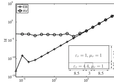
mode, the phase coefficient of which is known to depend lin-early on frequency in the LF regime. Fig. 4 gives results for both numerical methods. While theE-Bdata exhibit the ex-pected behavior, the phase coefficients produced by theA
-V method stagnate for frequencies below104Hz. This may
295
come as a surprise, because the latter formulation was de-signed to be low-frequency stable (Farle et al., 2004).
To clarify the situation, we present in Table 1 a compari-son for not only the quasi-TEM wave but also the first two
10−5 100 105 1010
10−15
10−10
10−5
100
105
Frequency in Hz
|
γ
|
EB AV
8.5 3 8.5
2 .2 5 9 .2 5
εr= 1,µr= 1
εr= 4.4,µr= 1
Fig. 4: Shielded microstrip line: LF behavior of propagation coefficient of quasi-TEM mode. Inset shows cross-section of structure. Dimensions are in mm.
Table 1: Comparison of first three modes of microstrip line
Mode Method 0Hz 10kHz 100kHz quasi- E-B 1.6653e-16 3.7160e-04j 3.7162e-03j
TEM A-V 4.7821e-04j 8.6431e-04 3.7630e-03j
Box 1 EA-B 1.5699e+02 1.5699e+02 1.5699e+02 -V 1.5699e+02 1.5699e+02 1.5699e+02
Box 2 EA-B 2.6987e+02 2.6987e+02 2.6987e+02 -V 2.6987e+02 2.6987e+02 2.6987e+02
box modes. It can be seen that only the quasi-TEM mode is
300
affected; the results for box modes are correct, even at 0 Hz. This behavior results from the fact that the static limit of|γ|is zero for the quasi-TEM mode but non-zero for all others. At sufficiently low frequency values,|γqTEM|becomes so much smaller than all other|γ|values that the eigenvalue solver is
305
unable to resolveγqTEMto sufficient accuracy, due to numer-ical noise. Note that the gap in eigenvalue|λ1/λ2|is
λ1 λ2 = γqTEM γBox 1
forE-Bmethod,
γqTEM γBox 1
2
forA-V method,
(55)
because the E-B formulation solves for γ and the A-V
310
scheme for γ2
. Fig. 5 presents the eigenvalue ratio as a function of frequency. For both formulations, the eigenvalue solver produces significant round-off error for |λ1/λ2|<
10−12
. . .10−9
. However, the frequency which this happens at is104
Hz for theA-V method, whereas the proposedE-B
315
scheme produces accurate results down to10−3Hz, thanks
to improved eigenvalue ratio in (55).
Figure 3. Convergence analysis for the TE10mode.
lossless case (σ=0) and in presence of Ohmic losses (σ = 5 S/m). Our main goal is to demonstrate the correct function of the present approach and compare it to theA−V potential formulation of (Farle et al., 2004), a state-of-the-art method that solves forγ2and models conductivity via complex per-mittivity, Eq. (1). According to (Pozar, 2005, p. 108), the an-alytical solution for the propagation coefficientγmnis given by
γmn= r
mπ a
2 +nπ
b 2
−εrµrk02+jµrσ k0η0, (54) where a and b denote the width and height of the wave-guide, respectively. Figures 1 and 2 present the dispersion curves of the TE10 and TE20 modes in the frequency range [10−10,1010]Hz, and Fig. 3b gives the error in propagation coefficient as a function of the number of unknowns.
In the lossless case, the solutions of both the E−B and
A−V methods are in very good agreement with the theory, over the whole frequency range; see Fig. 1. Figure 3a demon-strates that the convergence rates of both formulations are the same, forf = 0 Hz andf = 5 GHz, respectively.
In the lossy case (σ=5 S/m), it can be seen from Fig. 2 that the E−B approach works over the entire frequency range whereas theA−V scheme fails to converge below 10−8Hz, due to breakdown of Eq. (1). Above this threshold, the re-sults of both methods agree very well with analytical rere-sults. The numerical noise visible in Fig. 2b for phase coefficients of very small magnitude, Imγ <10−12rad/m, is insignifi-cant because, as seen in Fig. 2a, the corresponding attenua-tion coefficients are more than 14 orders of magnitude larger, Reγ >120. Figure 3b indicates that, within their respective range of validity, both numerical methods exhibit the same rate of convergence, independently of frequency. In case of theE−Bscheme, this also holds in the static case,f = 0 Hz. 4.2 Shielded microstrip line
The purpose of this example is to demonstrate the advan-tage of formulating the eigenvalue problem in terms of γ
R.Baltes et al.: Mixed Finite-Element Formulation for Electromagnetic Waveguides 5
102 104 106
10−5 10−4 10−3 10−2 10−1
Number of unknowns
| γAna − γNum | AV 0Hz EB 0Hz AV 5GHz EB 5GHz
(a) Lossless case:σ= 0S/m.
102 104 106
10−5 10−4 10−3 10−2 10−1
Number of unknowns
| γAna − γNum | EB 0Hz AV 1Hz EB 1Hz AV 5GHz EB 5GHz
(b) Lossy case:σ= 5S/m.
Fig. 3: Convergence analysis for the TE10mode.
[10−10,1010]Hz, and Fig. 3b gives the error in propagation
coefficient as a function of the number of unknowns. In the lossless case, the solutions of both theE-BandA
-265
V methods are in very good agreement with the theory, over the whole frequency range; see Fig. 1. Fig. 3a demonstrates that the convergence rates of both formulations are the same, forf = 0 Hz andf = 5 GHz, respectively.
In the lossy case (σ=5 S/m), it can be seen from Fig. 2
270
that theEBapproach works over the entire frequency range whereas theA-V scheme fails to converge below10−8Hz,
due to breakdown of (1). Above this threshold, the results of both methods agree very well with analytical results. The numerical noise visible in Fig. 2b for phase coefficients of
275
very small magnitude,Imγ <10−12
rad/m, is insignificant because, as seen in Fig. 2a, the corresponding attenuation coefficients are more than 14 orders of magnitude larger,
Reγ >120. Fig. 3b indicates that, within their respective range of validity, both numerical methods exhibit the same
280
rate of convergence, independently of frequency. In case of theE-Bscheme, this also holds in the static case,f= 0 Hz.
4.2 Shielded Microstrip Line
The purpose of this example is to demonstrate the advantage of formulating the eigenvalue problem in terms ofγ rather
285
thanγ2, with respect to round-off error in propagation
coef-ficients of small magnitude. Again, we compare theE-Band
A-V methods, by means of the lossless shielded microstrip line shown on the inset of Fig. 4. In contrast to the RWG of Section 4.1, the present structure supports a quasi-TEM
290
mode, the phase coefficient of which is known to depend lin-early on frequency in the LF regime. Fig. 4 gives results for both numerical methods. While theE-Bdata exhibit the ex-pected behavior, the phase coefficients produced by theA
-V method stagnate for frequencies below104
Hz. This may
295
come as a surprise, because the latter formulation was de-signed to be low-frequency stable (Farle et al., 2004).
To clarify the situation, we present in Table 1 a compari-son for not only the quasi-TEM wave but also the first two
10−5 100 105 1010
10−15
10−10
10−5
100
105
Frequency in Hz
|
γ
|
EB AV
8.5 3 8.5
2 .2 5 9 .2 5
εr= 1,µr= 1
εr= 4.4,µr= 1
Fig. 4: Shielded microstrip line: LF behavior of propagation coefficient of quasi-TEM mode. Inset shows cross-section of structure. Dimensions are in mm.
Table 1: Comparison of first three modes of microstrip line
Mode Method 0Hz 10kHz 100kHz quasi- E-B 1.6653e-16 3.7160e-04j 3.7162e-03j
TEM A-V 4.7821e-04j 8.6431e-04 3.7630e-03j
Box 1 AE-B 1.5699e+02 1.5699e+02 1.5699e+02 -V 1.5699e+02 1.5699e+02 1.5699e+02
Box 2 AE-B 2.6987e+02 2.6987e+02 2.6987e+02 -V 2.6987e+02 2.6987e+02 2.6987e+02
box modes. It can be seen that only the quasi-TEM mode is
300
affected; the results for box modes are correct, even at 0 Hz. This behavior results from the fact that the static limit of|γ|is zero for the quasi-TEM mode but non-zero for all others. At sufficiently low frequency values,|γqTEM|becomes so much smaller than all other|γ|values that the eigenvalue solver is
305
unable to resolveγqTEMto sufficient accuracy, due to numer-ical noise. Note that the gap in eigenvalue|λ1/λ2|is
λ1 λ2 = γqTEM γBox 1
forE-Bmethod,
γqTEM γBox 1
2
forA-V method, (55)
because the E-B formulation solves for γ and the A-V
310
scheme for γ2. Fig. 5 presents the eigenvalue ratio as a
function of frequency. For both formulations, the eigenvalue solver produces significant round-off error for |λ1/λ2|<
10−12. . .10−9. However, the frequency which this happens
at is104
Hz for theA-V method, whereas the proposedE-B
315
scheme produces accurate results down to10−3Hz, thanks
to improved eigenvalue ratio in (55).
Figure 4. Shielded microstrip line: LF behavior of propagation
co-efficient of quasi-TEM mode. Inset shows cross-section of structure. Dimensions are in mm.
rather thanγ2, with respect to round-off error in propaga-tion coefficients of small magnitude. Again, we compare the
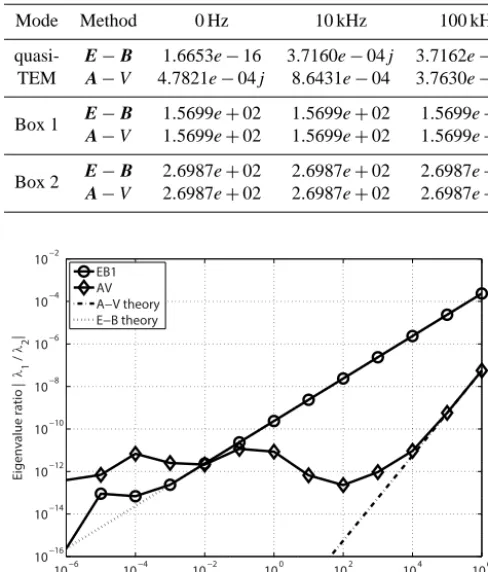
E−BandA−V methods, by means of the lossless shielded microstrip line shown on the inset of Fig. 4. In contrast to the RWG of Sect. 4.1, the present structure supports a quasi-TEM mode, the phase coefficient of which is known to de-pend linearly on frequency in the LF regime. Figure 4 gives results for both numerical methods. While theE−Bdata ex-hibit the expected behavior, the phase coefficients produced by theA−V method stagnate for frequencies below 104Hz. This may come as a surprise, because the latter formulation was designed to be low-frequency stable (Farle et al., 2004). To clarify the situation, we present in Table 1 a compari-son for not only the quasi-TEM wave but also the first two box modes. It can be seen that only the quasi-TEM mode is affected; the results for box modes are correct, even at 0 Hz. This behavior results from the fact that the static limit of|γ| is zero for the quasi-TEM mode but non-zero for all oth-ers. At sufficiently low frequency values,|γqTEM| becomes so much smaller than all other|γ|values that the eigenvalue solver is unable to resolveγqTEMto sufficient accuracy, due to numerical noise. Note that the gap in eigenvalue|λ1/λ2|is
λ1 λ2 = γqTEM
γBox 1
forE−Bmethod,
γqTEM
γBox 1
2
forA−V method,
(55)
because theE−Bformulation solves forγ and theA−V scheme forγ2. Figure 5 presents the eigenvalue ratio as a function of frequency. For both formulations, the eigenvalue solver produces significant round-off error for |λ1/λ2|< 10−12. . .10−9. However, the frequency which this happens at is 104Hz for the A−V method, whereas the proposed
18 R. Baltes et al.: Mixed finite-element formulation for electromagnetic waveguides
Table 1. Comparison of first three modes of microstrip line.
Mode Method 0 Hz 10 kHz 100 kHz
quasi- E−B 1.6653e−16 3.7160e−04j 3.7162e−03j
TEM A−V 4.7821e−04j 8.6431e−04 3.7630e−03j
Box 1 E−B 1.5699e+02 1.5699e+02 1.5699e+02
A−V 1.5699e+02 1.5699e+02 1.5699e+02
Box 2 E−B 2.6987e+02 2.6987e+02 2.6987e+02
A−V 2.6987e+02 2.6987e+02 2.6987e+02
10−6 10−4 10−2 100 102 104 106
10−16
10−14
10−12
10−10
10−8
10−6
10−4
10−2
Frequency in Hz
Eigenvalue ratio |
λ1
/
λ2
|
EB1 AV A−V theory E−B theory
Figure 5. Eigenvalue ratio versus frequency.
5 Critical discussion and conclusions
We have presented a mixed finite-element formulation for electromagnetic waveguides. Stability in the LF regime is achieved by imposing source-free conditions for the electric and magnetic flux densities, with the help of Lagrange mul-tipliers.
Since the sought eigenvalue is the propagation coefficient itself rather than its square, round-off errors in propagation coefficients of small magnitude are significantly reduced. This is of great practical importance for the mixed-signal analysis of transversally inhomogeneous transmission line structures, such as microstrips or coplanar waveguides: For the example of Sect. 4.2, the LF range is extended by 7 orders of magnitude, compared to γ2approaches. Another feature of the proposed method is that Ohmic losses enter the formu-lation directly rather than in the form of equivalent complex permittivity.
The advantages of the new method do not come for free, though. Table 2 shows that the number of variables is three times as large as in the A−V case. Nevertheless, the non-zeros inAˆ+ ˆC just increase by 50 %, and those inB actuallyˆ decrease. Iteration counts of theeigssolver of MATLAB-R2013a are 50 % higher for theE−Bapproach. As a result, solution times for the lossy RWG are six times as long. For the microstrip, that ratio is twelve because, in the lossless
Table 2. Computational data.
Example Lossy RWG Microstrip
Method E−B A−V E−B A−V
Unknowns 11074 3969 13377 4416
Non-zerosAˆ+ ˆC 73707 60167 107496 70602
Non-zerosBˆ 19844 34375 29328 39386
Runtime in sec 1.52 0.27 2.96 0.24
Iterations 85 59 82 55
case, the system matrices of theA−V method become real-valued, whereas those of theE−Bscheme remain complex.
Acknowledgements. This work was supported in part by grant DY
112/1-1 of the Deutsche Forschungsgemeinschaft (DFG).
Edited by: U. van Rienen
Reviewed by: two anonymous referees
References
Bardi, I. and Biro, O.: An efficient finite-element formulation with-out spurious modes for anisotropic waveguides, IEEE T. Microw. Theory, 39, 1133–1139, 1991.
Bertazzi, F., Peverini, O. A., Goano, M., Ghione, G., Orta, R., and Tascone, R.: A fast reduced-order model for the full-wave FEM analysis of lossy inhomogeneous anisotropic waveguides, IEEE T. Microw. Theory, 50, 2108–2114, 2002.
Boffi, D., Brezzi, F., and Fortin, M.: Mixed Finite Element Methods and Applications, Spinger, Berlin, 2013.
Farle, O., Hill, V., and Dyczij-Edlinger, R.: Finite-Element Wave-guide Solvers Revisited, IEEE T. Magn., 40, 1468–1471, 2004. Hiptmair, R., Krämer, F., and Ostrowski, J.: A Robust Maxwell
Formulation for All Frequencies, IEEE T. Magn., 44, 682–685, 2008.
Lee, J.-F.: Finite Element Analysis of Lossy Dielectric Waveguides, IEEE T. Microw. Theory, 42, 1025–1031, 1994.
Lee, J.-F., Sun, D. K., and Cendes, Z. J.: Full-Wave Analysis of Dielectric Waveguides Using Tangential Vector Finite Elements, IEEE T. Microw. Theory, 39, 1262–1271, 1991.
Lee, S.-C., Lee, J.-F., and Lee, R.: Hierarchical vector finite ele-ments for analyzing waveguiding structures, IEEE T. Microw. Theory, 51, 1897–1905, 2003.
Polstyanko, S. V. and Lee, J.-F.: H1(curl) Tangential Vector
Fi-nite Element Method for Modeling Anisotropic Optical Fibers, J. Lightwave Technol., 13, 2290–2295, 1995.
Polstyanko, S. V., Dyczij-Edlinger, R., and Lee, J.-F.: Fast Fre-quency Sweep Technique for the Efficient Analysis of Dielectric Waveguides, IEEE T. Microw. Theory, 45, 1118–1126, 1997. Pozar, D. M.: Microwave Engineering, 3rd Edition, John Wiley &
Sons, New York, 2005.
Schultschik, A., Farle, O., and Dyczij-Edlinger, R.: A Model Order Reduction Method for the Finite-Element Simulation of Inhomo-geneous Waveguides, IEEE T. Magn., 44, 1394–1397, 2008. Valor, L. and Zapata, J.: Efficient Finite Element Analysis of
Char-R. Baltes et al.: Mixed finite-element formulation for electromagnetic waveguides 19
acterized by Arbitrary Permittivity and Permeability Tensors, IEEE T. Microw. Theory, 43, 2452–2459, 1995.
Vardapetyan, L. and Demkowicz, L.: Full-wave analysis of dielec-tric waveguides at a given frequency, Math. Comput., 72, 105– 129, 2003.