1Microelectronics Department, Brandenburg University of Technology, 03046 Cottbus, Germany 2IHP, Im Technologiepark 25, 15236 Frankfurt (Oder), Germany
Correspondence to:Dirk Killat ([email protected]) and Stefan Bramburger ([email protected])
Received: 9 January 2017 – Revised: 23 May 2017 – Accepted: 9 July 2017 – Published: 21 September 2017
Abstract.This paper presents a modified interpolation algo-rithm for signals with variable data rate from asynchronous ADCs. The Adaptive weights Conjugate gradient Toeplitz matrix (ACT) algorithm is extended to operate with a contin-uous data stream. An additional preprocessing of data with constant and linear sections and a weighted overlap of step-by-step into spectral domain transformed signals improve the reconstruction of the asycnhronous ADC signal. The interpo-lation method can be used if asynchronous ADC data is fed into synchronous digital signal processing.
1 Introduction
An approach to improve the energy efficiency of ADCs is their asynchronous operation: The ADC is operated with a variable clock depending on the characteristics of the input signal. The average power consumption of the ADC and the power required for RF data transmission is reduced with a reduction of the average sample rate. Asynchronous ADCs are potentially applicable in stand-alone sensor nodes, bio-medicine (Yuan and Lam, 2013) or energy management.
The drawback of an asynchronous operation is the vari-able data rate which needs to be synchronized to the clock of the subsequent signal processing system by interpola-tion. Several methods exist for interpolation; some operate in time domain (Neubauer, 2003), others in frequency do-main (Feichtinger et al., 1995). The interpolation algorithms differ considerably in complexity and the quality of the re-constructed signal.
The base for the presented interpolation algorithm is the Adaptive weights Conjugate gradient Toeplitz matrix (ACT) algorithm. It operates in the frequency domain and has the drawback of much higher computational effort than interpo-lation in the time domain, but it converges much faster than
other frequency domain based interpolation algorithms (Uni-versity of California, 2016).
The simulation data is based on a tracking ADC (Fig. 1). The output data rate is variable because it depends on the input signal characteristics. The difference between the cur-rent input signal and the output of the I-DAC controls the ADC clock rate. If the difference gets larger the clock rate is increased. The resulting datastream output is used for the interpolation.
This work is organized as follows: Sect. 2 briefly explains the basic principle of the ACT algorithm, Sect. 3 describes the extensions to the ACT algorithm, Sect. 4 presents simu-lation results and Sect. 5 concludes the paper.
2 ACT-algorithm
The ACT algorithm requires high computational effort be-cause it uses several mathematical methods (Feichtinger et al., 1995). The first is the adaptive weights method (Neubauer, 2003) in which the weights of the points are cal-culated according to Eq. (1). This input weighting vectorwj
is used to calculate the spectral transformation of the time of the samples (Eq. 2). The parameterM denotes the number of spectral lines of the input signal and results from the ratio of the largest time distance between two sample points and the shortest time distance between two sample points. The amplitude valuesp(tj)are transformed into spectral domain using the weighting vectorwj(Eq. 3).
wj=
tj+1−tj−1
2 ; J∈ {1,2, . . ., J} (1)
yk= J
X
j=0
Figure 1.Asynchronous tracking ADC as signal source for interpolation algorithm.
bk= J
X
j=0
p tj·wj·e−i2π ktj; |k| ≤M (3)
The next step in the ACT algorithm is the construction of the Toeplitz matrixTw (Eq. 4). The property of the Toepliz
matrix are constant values on each descending diagonal. Ad-ditionally the values above the descending main diagonal are complex conjugate of the values below the diagonal. These properties make the calculations in the subsequent iterative process very efficient (University of California, 2016).
Tw=
y0 y1 . . . y2M−1 y2M y1 y0 . . . y2M−2 y2M−1
. . . .. . . . y2M−1 y2M−2 . . . y0 y1
y2M y2M−1 . . . y1 y0 (4)
The spectrum of weighted time valuesyk, the weighted spec-trum of amplitude valuesbk and the toeplitz matrix are used
to solve Eq. (5) for the interpolated spectrum a. b is set tobk. This equation will be solved iteratively with the help
of the conjugate gradient method (Eq. 6). In combination with the Toeplitz matrix the system converges quickly and after a maximum of 2M+1 iteration loops the result is avail-able. The initial parameters of the system are these:an−1=0,
rn−1=bkandqn−1=bk.
Tw·a=b (5)
an=an−1+
rn−1,qn−1
Twqn−1,qn−1 ·qn−1
rn=rn−1−
rn−1,qn−1
Twqn−1,qn−1
·Twqn−1
qn=rn−
rn,Twqn−1
Twqn−1,qn−1
·qn−1 (6)
Finally the interpolated spectrumak is transformed back to
the time domain with Eq. (7) using an arraytwith equidistant time steps of the interpolated signal.
p(t )= M
X
k=−M
ak·ei2π kt (7)
3 Extension to ACT algorithm
Frequency based interpolation can be used on signals of a fi-nite period because the number of sample points for the DFT is limited. To deal with a continuous data stream the data has to be split into equally spaced sections. Every section can now be interpolated for itself and the interpolated data stream is constructed by connecting the interpolated sections. 3.1 Smooth transition between sections
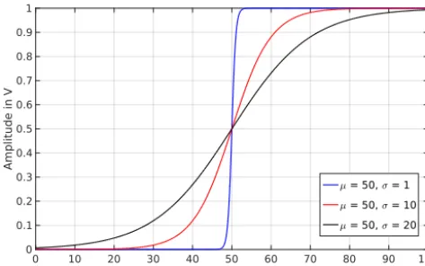
By connecting the interpolated sections undesired steps in amplitude can occur at the transitions of the sections. This problem can be solved by overlapping the boundaries of the sections by a certain amount of samples. Further improve-ment is achieved by using a smoothing function on the over-lapping areas. Here the hyperbolic tangent function as pro-posed in Rädler (2016) is used. Advantages of this transition function is scalability of slope and good convergence to final values. The multiple derivative hyperbolic tangent is continu-ous, which is advantageous in subsequent signal processing. The smoothness of the merging of two sections is deter-mined by σ. The higher the value of σ the smoother the transition is. But with a higherσ the function needs more samples for overlapping. Figure 2 shows the used smoothing functions with a total overlap of 100 samples and different grades of smoothness.
The merger of two sections using the smoothing function is exemplified by Eq. (8). The parameterµ determines the transition point between both sections.
pmerged(t )=p2(t )· 1
2+ 1 2tanh
t−µ
σ
+p1(t )· 1− 1 2+ 1 2tanh
t−µ
σ
Figure 2.Hyperbolic tangent function for smoothing transitions be-tween sections of samples of data stream.
3.2 Amplitude shifting function
Another issue of interpolation is the boundary-value prob-lem: The first value and the last value of a section should have the same level. But this occurs either very rarely or not at all for arbitrary input signals. This results in significant interpolation errors at the section boundaries. The proposed solution is a transformation of the input signal by a linear function as described by Eq. (9) before the application of the interpolation algorithm. The whole section of the signal is shifted by the amplitude value of the first point of the signal to zero. In addition a linear function is added so that the last sample point is zero as well.
ptransform tj
=p tj
−ϑ· tj−t1−p(t1)
withϑ=p(tJ)−p(t1) tJ−t1
(9) In Fig. 3 the linear function (gradient) is drawn in black. The linear function is alined to the first and the last value of the input signal (blue). The transformed signal (red) has its first and last point on zero level. After interpolation in the fre-quency domain the inverse transformation has to be applied to retrieve the original signal.
3.3 Signals with sporadic constant sections
The interpolation algorithm should be suitable for all kind of signal shapes. Critical points are signals with sporadic con-stant sections, e.g. a square wave signal as shown in Fig. 4. At the left side the interpolated signal (blue) does not repre-sent the original signal (red). On the right side the edges are interpolated well but large overshoots exist. The reason for this difference between both interpolations is the cutoff fre-quencyMof the input signal. The higherMthe higher the
frequencies; respectively more spectral linesM(Eq. 11) are used for the interpolation. To change the number of spectral lines Mthat are used for calculation the factor κ has to be varied. Factorκis used to calculateMin Eq. (10).
0 0.1 0.2 0.3 0.4 0.5 0.6 0.7 0.8 0.9 1
Time in s (normalized)
Figure 3.Transformation of input signal of one section to set first and last data point to zero.
M must be set in relation to the minimum bandwidth
of the original signal. ThereforeM is calculated from the
maximum sample step sizeTmaxby introducing the factorκ (Eq. 10). This factor has a range between 0 and 1. The higher κ is, the better the interpolation of the slopes of a square wave signal. The number of spectral lines for inter-polation depends onM (Eq. 11).
M =κ· π Tmax
; 0< κ <1 (10)
M=
M·N·Tmin
π
+1 (11)
The reason for overshoots in the right part of Fig. 4 is the small number of samples from the asynchronous ADC that is used as input for interpolation. An ideal asynchronous ADC produces samples only at transitions of rectangular wave-form. The solution is to synthetically fill the constant sections with additional samples. The sections that have to be filled with additional samples before interpolation are detected by the variation of the distance of two successive sample points (Eq. 12). A change of the distance between two successive time steps by a factor greater thanτ (Eq. 12), resulting in additional samples being introduced.
tj+2−tj+1
> τ· tj+1−tj
(12) The factorτ has to be chosen carefully so that the fill algo-rithm will be activated during constant sections of a square wave signal or arbitrary signal but not at low frequent sine waves input. The activation depends on the sample rate algo-rithm of the asynchronous ADC.
4 Results
Figure 4.Result of interpolation of rectangular waveform with asynch. ADC samples only at transitions; low cutoff (κ=0.3) and high cutoff (κ=0.8) frequency for interpolation.
Figure 5.Comparision of time domain and frequency domain based interpolation (ACT) with original signal (red) and asynchronous ADC output (x).
second derivative is at its maximum and the asynchronous ADC produces the largest errors compared to original signal. Therefore the peak of the sinus is well suited to demonstrate the effectiveness of the interpolation algorithm. The origi-nal sine wave (red) and the output of the asynchronous ADC (1q=0.01) are given as well. In fact the spline interpolated function is exactly in line with sampled ADC data, but the ACT interpolation result (black) fits best with the original signal.
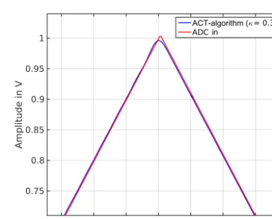
Figure 6 shows the interpolation of a triangle signal. The falling and rising slopes are interpolated well, but the vertex is flattened because of the reduced sample rate of the asyn-chronous ADC before the vertex.
The effectiveness of synthetic insertion of additional sam-ple points in a square wave signal is depicted in Fig. 7. The reduced sample rate of the asynch. ADC at the rising slope of the rectangular signal and the quantization levels produces an
ACT-algorithm ( i
Figure 6.Interpolated triangle waveform from asynch. ADC.
ACT-algorithm (
ACT-algorithm (i
Figure 7.Interpolation of asynch. ADC samples with rect. wave-form.
error that is larger than the interpolation error. The overshoots due to interpolation are reduced to a minimum through the filling of the constant sections. Ringing only exists at the be-ginning and at the end of the section depending on the band-width of the interpolation algorithm.
inter-104 105 106 Frequency in Hz
10-8
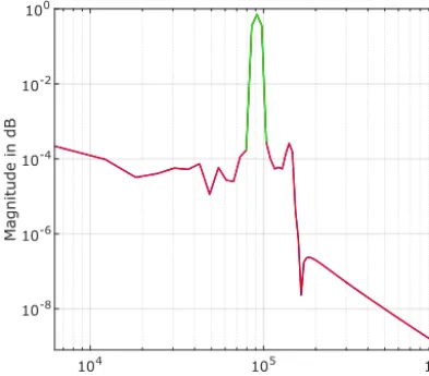
Figure 8.Spectrum of an interpolated sine wave:f=91 kHz, res-olution n=8 bit, sample rate of asynch. ADC variable between 2.8 and 25 MS s−1, interpolation bandwidth G=140 kHz, fre-quency resolution1f=6.1 kHz.
polated signal is shown in Fig. 8. By reducing the interpo-lation cutoff frequency G to 140 kHz, a full scale
resolu-tion of 8 bits and a sample rate varying between a minimum of 2.8 MS s−1 and a maximum of 50 MS s−1, an SNDR of 65 dB can be achieved, which is remarkable far above the SNDR of 43 dB that would have been achieved with cubic spline interpolation. The stepsize of the simulated Tracking ADC is 1 or 2 LSB per clock cycle. The results can be inter-preted as follows: An interpolation in the frequency domain with interpolation cutoff frequency increases the signal res-olution by oversampling. To achieve an optimal SNDR it is important to know the signal waveform that has to be pro-cessed. E.g. for a sinus the value ofκcould be lower than for a rectangular waveform.
Frequency based interpolation is well suited for filtering of noise (Fig. 9). This can demonstrated by feeding a si-nusoidal input with a noise ripple of 10 pW Hz−1 into the asynch. ADC input. As the peak value of signal plus noise is limited to 1 V the interpolated sinusoidal signal (blue) has a smaller amplitude than the ideal one (black).
Table 1 gives an overview of the computation time and mean deviations of the ACT algorithm in comparison to stan-dard adaptive weights interpolation and Fourier series expan-sion using the program Matlab. For a sinusoidal input the ACT algorithm interpolates much faster than the other meth-ods. The speed of interpolation depends on the number of points given and the number of spectral lines used for cal-culation. A square wave signal requires more computation time than a sinusoidal signal. Fourier series expansion does not converge in a reasonable time in the case of a square wave signal. The length of the interpolated signal of the waveforms given in Table 1 is 0.025 ms. This interpolation, performed withMatlab, is not suitable for real-time processing at such
2.35 2.4 2.45 2.5 2.55 2.6 2.65
Time in s #10-5 0.88
0.9 0.92 0.94 0.96 0.98 1
Ampl
itude in V
Ideal sine wave ADC out
Figure 9.Interpolation result (blue) of sinusoidal ADC input with noise.
a high input sampling rate and signal bandwidth. But for low data rate signals e.g. for biomedical applications or environ-mental sensors, real-time processing may become feasible.
5 Conclusions
In this work the practical implementation of frequency do-main interpolation of asynchronous ADC data using the ACT algorithm (Feichtinger et al., 1995) is demonstrated. The continuous data stream is split into sections for individual interpolation in the frequency domain. The original ACT al-gorithm is improved in three steps: firstly DC offset and 1st-order linear contribution are removed from the original function. Secondly the individual interpolated sections are reassembled using a smoothing function. Thirdly the prob-lem of periods with reduced sample rate due to asynchronous ADC sampling is eliminated by synthetic insertion of sam-ples before interpolation.
inter-polation algorithm related to the frequency resolution control the amplitude resolution and ratio of noise suppression.
Both the synthetic insertion of samples in the data stream, the optimal segmentation of data stream before spectral in-terpolation, as well as the optimal adjustment of interpola-tion bandwidth in relainterpola-tion to the minimum ADC sample rate and signal bandwidth, depend on the algorithm of the asyn-chronous ADC. A feedback from signal processing analyz-ing the interpolated signal waveform to the control of inter-polation algorithm parameters have the potential for further improvements of interpolation of asynchronous ADC data.
Data availability. Tracking ADC simulation results used to get in-terpolation results of Figs. 4, 5, 8 and 9 are available in the Supple-ment.
The Supplement related to this article is available online at https://doi.org/10.5194/ars-15-163-2017-supplement.
Competing interests. The authors declare that they have no conflict of interest.
Acknowledgements. The authors thank the German Research Community (DFG) for funding the project under grant num-ber KI 1585/2-1.
Edited by: Jens Anders
Reviewed by: two anonymous referees
Feichtinger, H. G., Gröchenig, K., and Strohmer, T.: Efficient nu-merical methods in non-uniform sampling theory, Numer. Math., 423–440, 1995.
Neubauer, A.: Irreguläre Abtastung: Signaltheorie und Signalverar-beitung, Springer, Berlin, Heidelberg, 2003.
NI – National Instruments: Schnelle Fourier-Transformation (FFT) und Fensterung, http://www.ni.com/white-paper/4844/de/, last access: 30 December 2016.
Rädler, J.: Smooth transition between functions with tanh(), https://www.j-raedler.de/2010/10/ smooth-transition-between-functions-with-tanh/, last access: 30 December 2016.