BioMedCentral
Methodology
BMC Medical Research Methodology 2001,
1 :8
Research article
On the probability of cost-effectiveness using data from randomized
clinical trials
Andrew R Willan
1
Address: 1Department of Clinical Epidemiology and Biostatistics, HSC-2C, McMaster University, 1200 Main Street West, Hamilton, ON, L8N 3Z5, Canada and 2The Centre for Evaluation of Medicines, St. Joseph's Hospital, Hamilton, ON, Canada
E-mail: [email protected]
Abstract
Background: Acceptability curves have been proposed for quantifying the probability that a treatment under investigation in a clinical trial is cost-effective. Various definitions and estimation methods have been proposed. Loosely speaking, all the definitions, Bayesian or otherwise, relate to the probability that the treatment under consideration is cost-effective as a function of the value placed on a unit of effectiveness. These definitions are, in fact, expressions of the certainty with which the current evidence would lead us to believe that the treatment under consideration is cost-effective, and are dependent on the amount of evidence (i.e. sample size).
Methods: An alternative for quantifying the probability that the treatment under consideration is cost-effective, which is independent of sample size, is proposed.
Results: Non-parametric methods are given for point and interval estimation. In addition, these methods provide a non-parametric estimator and confidence interval for the incremental cost-effectiveness ratio. An example is provided.
Conclusions: The proposed parameter for quantifying the probability that a new therapy is cost-effective is superior to the acceptability curve because it is not sample size dependent and because it can be interpreted as the proportion of patients who would benefit if given the new therapy. Non-parametric methods are used to estimate the parameter and its variance, providing the appropriate confidence intervals and test of hypothesis.
Introduction
In reporting cost-effectiveness analyses alongside clini-cal trials, authors [1–4] have used various definitions, es-timation methods and interpretations for acceptability curves. Acceptability curves provide an excellent means of quantifying the stochastic uncertainty of the estimated incremental cost-effectiveness ratio (ICER) in relation to a particular value ascribed to a unit of effectiveness. It is the certainty, expressed as a probability, that the current evidence would lead us to believe that some new therapy
is cost-effective, insofar as the ICER is less than the value ascribed to a unit of effectiveness. In addition, accepta-bility curves provide an estimator for the ICER and its confidence limits. However, acceptability curves are of-ten interpreted and expressed as the probability that the new therapy is cost-effective. It is argued below that this is subject to misinterpretation, and an alternative defini-tion for a parameter representing the probability that the new therapy is cost-effective is introduced. Data from a clinical trial can be used to make statistical inference Published: 6 September 2001
BMC Medical Research Methodology 2001, 1:8
Received: 23 May 2001 Accepted: 6 September 2001
This article is available from: http://www.biomedcentral.com/1471-2288/1/8
about this parameter. Furthermore, the inference pro-vides a non-parametric estimator for the ICER and its confidence interval.
In a two-arm randomized control trial let eji and cji be the respective measures of effectiveness and cost for patient i on therapy j, where j = T (treatment), S (standard); i = 1, 2, . . .nj ; and nj is the number of patients randomized to therapy j. Typically, eji is the patient's survival time (perhaps quality-adjusted) from randomization to death or to the end of the period of interest. Let
. Define c similarly.
Let E( e) = ∆e and E( c) = ∆c, where E is the expecta-tion funcexpecta-tion. Thus, the incremental cost-effectiveness
ratio (ICER) is ∆c/∆e, and is estimated by c / e. In addition, the incremental net benefit [5–9] (INB) is ∆eλ
-∆c, and is estimated by eλ - c, where λ is the value given to a unit of effectiveness. Typically the INB is ex-pressed as a function of λ, allowing readers to provide the value they consider most relevant.
van Hout et al. [1] define the acceptability curve as "the probability that the [ICER] is under a certain acceptable limit", say λ. The acceptability curve, then, is a function of λ. If one assumes that the authors are referring to the true ICER ratio, the definition is Bayesian. In the same paper they define the acceptability curve in algebraic
terms as , where f is the
joint probability density function for the random vector
( e, c)'. Here the definition is not Bayesian, since it is the probability that, in repeated sampling, the random
variable eλ - c (i.e., the observed net benefit) is greater than 0. In an illustration, the authors substitute the sample estimates for the model parameters in f to
yield an empirical density function, call it , and refer to the acceptability curve as the probability that the ICER is acceptable. Briggs and Fenn [2] refer to the acceptability curve as "the probability an intervention is cost-effective in relation to different values of" λ. For estimation they
propose using the integration of , as above, or deter-mining the proportion of bootstrap re-samples in which
eλ - c is greater than 0.
Briggs[3] provides a purely Bayesian approach by defin-ing the acceptability curve as the probability that ∆eλ - ∆c is greater than 0. In an illustration the author interprets the acceptability curve as "probability of cost-effective". Assuming f is the density function for a bivariate normal random vector, and using an uninformative prior, the
ac-ceptability curve is given by A(λ)= g(x)dx, where g is
the probability density function for a normal random
variable with mean eλ - c and variance
, where and
are estimates of the variance of eji and cji,
respective-ly, and is an estimate of the correlation between eji and cji . This is exactly the same curve as determined by the
integration of , given above, and, due to the symmetry, is equal to 1 minus the p-value of the test of the hypothe-sis ∆eλ - ∆c < 0. In reporting the results of a cost-effec-tiveness analysis, Raikou et al. [4] interpret the acceptability curve as the "probability that intervention is cost effective".
By rewriting Pr(∆eλ - ∆c > 0) as Pr(∆c/∆e < λ), assuming ∆e > 0, the acceptability curve can be interpreted as the posterior distribution for the ICER. Defining A(λγ) = γ, the estimate for the ICER and its (1-α/2)100% Baysian limits are given by λ0.5, λα/2 and λ1-α/2, respectively.
The interpretation that the acceptability curve is the probability that the intervention is cost-effective is not entirely accurate and could easily be misunderstood by policy makers. Consider the situation in which the ob-served INB for treatment is very small, but due to a very large sample size the acceptability curve at the value of λ of interest is 0.99. Attaching the label "the probability that the intervention is cost-effective" to this quantity could mislead policy makers into thinking that treatment is highly beneficial compared to standard. What, in fact, is high is our confidence that the INB, however small, is not zero. A more accurate interpretation of the accepta-bility curve is that it is a measure of the certainty with which the current evidence would lead us to believe that treatment is cost-effective, i.e., ∆eλ - ∆c > 0. For a Baye-sian, this is Pr(∆eλ - ∆c) > 0, and for a frequentist, it is, assuming symmetry, 1 minus the p-value for the test of the hypothesis ∆eλ - ∆c < 0. This is not just the traditional confusion between statistical and clinical significance. In significance testing as the sample size increases, the
var-et
∆
^
.
e T
Ti i n
S Si i
n
n
e
n
e
T S
=
−
= =
∑
∑
1
1
1 1
-
^
c-
^
c-
^
c-
^
c-
^
c-
^
c-
^
cas
A
f e c dc de
e
( )
λ
( , )
,
λ
=
−∞ −∞
∞
∫
∫
^
^
-
^
-
c^
c-
^
c-
^
cf f
^
,
f f
^
,
-
^
c-
^
cg
∞∫
0
-
^
c-
^
ce
1
2 2 22
n
jj S T
j j j j j
=
∑
+ −
,
^ ^ ^ ^ ^
,
σ λ ω
σ ω ρ λ
^
e
)
^
2 jd
7
^
2jd
'
^
jiance of the estimator decreases, but the magnitude of the parameter being estimated stays the same. However, as sample size increase the magnitude of the acceptabili-ty curve for a given λ increases.
In the next section we provide a more accurate definition for the probability that treatment is cost-effective. The definition contains no element of certainty, and is the probability of the "next" patient realizing a larger net benefit if he or she is given treatment rather than stand-ard. Using data from a clinical trial, non-parametric methods can be used to estimate this probability, and uncertainty
Methods
The probability that treatment is cost-effective
Let bji(λ) = ejiλ - cji. The quantity bji(λ) is the net benefit, expressed in money, realized by patient i on therapy j. An alternative to the acceptability curve for quantifying the probability that treatment is cost-effective is defined as: θ(λ) ≡ the probability, for a given λ, that a patient will re-ceive a larger net benefit with treatment rather than standard. Its definition is not Bayesian because it is a probability statement about random variables, not pop-ulation parameters. Nonetheless, it relates directly to the notion of the probability of treatment being cost-effec-tive. A policy maker can genuinely interpret θ(λ) as the probability of the "next" patient realizing a larger net benefit if he or she is given treatment rather than stand-ard. Such a direct interpretation is not provided by the acceptability curve. The acceptability curve is the proba-bility that the average net benefit of a group of patients of the same size as in the clinical trial will be greater is they receive treatment rather than standard.
To estimate θ(λ) we borrow methodology from receiver operating characteristic curves [10]. An estimate of θ(λ) is given by:
If there are no ties, (λ) is the proportion of all the pos-sible comparisons of a patient on treatment with a pa-tient on standard in which the former was observed to have a larger net benefit. The estimate of the variance of
(λ), denoted by , is given by:
The 100(1 - α)% confidence interval, defined as
(λ)±sθ(λ)z1-α/2, can be used to express the uncertainty
regarding (θ), where Z1-α/2 is the 100(1 - α/2)th per-centile of the standard normal distribution. We have
made the assumption that in large samples (λ) will be normally distributed.The value λ0.5, defined at θ (λ0.5) = 0.5, provides a non-parametric estimator of the ICER, since it is that value of λ for which treatment and stand-ard are equally cost-effective in the sense that Pr [bTk(λ0.5) > bSi(λ0.5)] = 0.5. The quantities λL and λU,
defined as (λL)+ sθ(λL)Z1-α/2 = 0.5 and (λU )-sθ(λU)Z1-α/2 = 0.5, respectively, are the corresponding lower and upper non-parametric confidence intervals for the ICER.
The hypothesis H0: θ (λ) = 0.5 versus H1: θ (λ) > 0.5 can
be tested at the level α by rejecting H0 if .
Rejecting H0 leads to the conclusion that the data pro-vide epro-vidence that treatment is cost-effective.
Suppose there is an interest in comparing θ (λ) between patient subgroups, say between males and females. To
achieve this, let M(λ) and F(λ) be the estimator of θ (λ) for males and females, respectively, with
correspond-ing estimated variances, and . Then the hypothesis that θ (λ) is the same for males and females can be rejected, at the α-level, 2-sided, if
There is an important distinction to be made between
A(λ) and (λ). As sample size increases, A(λ) approach-es 1 if ∆eλ - ∆c > 0, reflecting the certainty that treatment is cost-effective. If ∆eλ - ∆c≤ 0, A(λ) approaches 0, re-flecting the certainty that treatment is not cost-effective.
The quantity (λ), being independent of sample size, ap-proaches θ(λ) regardless of ∆eλ - ∆c. The certainty with which θ(λ) is estimated is reflected in sθ(λ) which is a de-creasing function of the sample size.
(
)
θ λ^( ) ψ ( ),λ ( ) ,λ ψ( , ) : : : . = = > = < = =
∑
∑
1 1 0 1 1 1 2n n b b where x y
y x y x y x
S T k
n i n Si Tk T S ^
s,
^
(
s,
^
(
y s
2(
),
(
)
s
n nS S nT k bSi bTk
n
i
nS T
θλ ψ λ λ θ λ
2 1 1 2 1 1 1 ( ) ( ) ( ), ( ) ( ) ^ = − − = =
∑
∑
(
)
+ − − = =∑
∑
1 1 1 1 1 2nT nT nS i bSi bTk
n
k nT S
( ) ( ), ( ) ( ) .
^
ψ λ λ θ λ
s,
^
(
s,
^
(
s,
^
(
s,
^
(
s,
^
(
s,
^
(
s,
^
(
s, s
M2(
) a d s
2 F(
).
s,
^
(
Example
In a trial of symptomatic hormone resistant prostate cancer [11,12], 161 patients were randomized between prednisone alone (S) and prednisone plus mitoxantrone (T). Although there was no statistically significant differ-ence in survival, there was better palliation with T. Cost data, including hospital admissions, outpatient visits, in-vestigations, therapies and palliative care, were collected retrospectively on the 114 patients from the three largest centres. Survival was quality-adjusted using the EORTC quality of life questionnaire QLQ-C30. All patients were followed until death. The sample means and the sample variance-covariance information can be found in Table 1. Cost is given in Canadian dollars (CAD$) and effective-ness in quality-adjusted life-weeks (QALW).
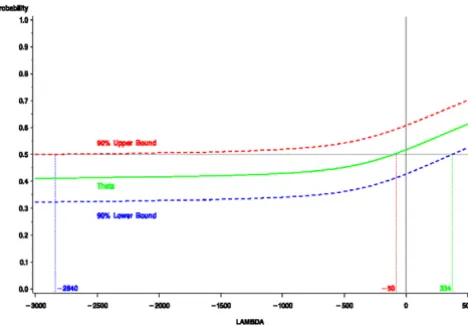
A plot of (λ), complete with 90% confidence intervals can be found in Figure 1. In this example all three plots have positive slope over the range of λ shown, although this would not be true for all examples. For example, by definition θ (0) = Pr(cTk - cSj < 0) and θ (λ) approaches Pr(eTk - eSj > 0) as λ becomes arbitrarily large, for any k and j. Therefore, any example in which Pr(cTk - cSj< 0) > Pr(eTk - eSj > 0) will have negative slope for some interval
of positive λ. In the prostate example, since (λ) crosses the 0.5 horizontal at λ = 50, for any value greater than
-50, the estimate of (λ) is greater than 0.5. The value -50 is a non-parametric estimate of the ICER, since for that value of λ, treatment and standard are equally cost-effective, in that the probability that a patient on treat-ment has the same net benefit as a patient on standard is 0.5. This compares to the parametric estimate of -134.
Since the lower bound crosses the 0.5 horizontal at 334, for any value greater than 334 the hypothesis θ(λ) < 0.5 can be rejected at the 5% level of significance. Thus, a non-parametric upper bound of the ICER is 334. This compares to 378 using Fieller's theorem [13,14]. For this
example a health policy maker can interpret the results as follows: for any positive λ, the estimated probability that treatment is cost-effective is greater than 50%; and for any λ greater than 334 per QALW, the probability that treatment is cost-effective is statistically significant-ly greater than 50%.
Discussion
As an alternative to the acceptability curve, the quantity θ(λ) is proposed as a definition for the probability that treatment is cost-effective. One advantage is that it is not sample size dependent, i.e. it is a population parameter. Another is that it has an appropriate interpretation, namely, it is the proportion of patients that realize a larg-er net benefit if given treatment rathlarg-er than standard. The acceptability curve does not provide this, although the language often used regarding it, implies that it does. The use of θ(λ) should be helpful to policy makers, since it does not confuse the magnitude of the benefit with the certainty of its estimate.
Analysis regarding the quantity θ(λ) is not proposed as an alternative to traditional cost-effectiveness analysis Table 1: Sample sizes and parameter estimates for prostate example
nj
average
effectiveness average cost
Standard 53 28.1 29039 16.4 7,872,681 2,876
Treatment 61 40.9 27322 24.1 6,466,351 2,771
)
^
2j
/n
j7
^
2j
/n
j'
^
j
)
^
j
7
^
j
/n
js,
^
(
s,
^
(
s,
^
(
Figure 1
Publish with BioMed Central and every scientist can read your work free of charge
"BioMedcentral will be the most significant development for disseminating the results of biomedical research in our lifetime."
Paul Nurse, Director-General, Imperial Cancer Research Fund
Publish with BMCand your research papers will be:
available free of charge to the entire biomedical community
peer reviewed and published immediately upon acceptance
cited in PubMed and archived on PubMed Central
yours - you keep the copyright
[email protected] Submit your manuscript here:
http://www.biomedcentral.com/manuscript/
BioMedcentral.com for allocating health care resources. When allocating a
fixed amount of resources to one of two new treatments, the proportion of patients receiving an increase in net benefit would be maximized by choosing the treatment with the larger θ(λ) to ∆c ratio. However, this would not maximize net benefit, since the ratio may be larger only because the between-patient variability in cost and effec-tiveness is smaller, resulting in a larger θ(λ).
Non-parametric methods can be used to estimate θ(λ) and its variance. This provides the appropriate confi-dence intervals and test of hypothesis. In addition, non-parametric estimates of the ICER and its confidence in-tervals can be determined. This is of particular impor-tance in the presence of highly skewed cost data.
Competing interests None declared.
Acknowledgements
The author wishes to acknowledge the reviewers whose comments led to a much improved manuscript and to thank Gary Foster for help with the figure.
References
1. van Hout BA, Al MJ, Gordon GS, Rutten EFH: Cost, effects and C/ E-ratios alongside a clinical trial.Health Economics 1994, 3 :309-319
2. Brigg A, Fenn P: Confidence intervals or surfaces? Uncertainty on the cost-effectiveness plane.Health Economics 1998, 7 :723-740
3. Briggs AH: A Bayesian approach to stochastic cost-effective-ness analysis.Health Economics 1999, 8:257-261
4. Raikou M, Gray , Briggs , Stevens A, Cull C, McGuire A, Fenn P, Strat-ton I, Holman R, Turner R: Cost effectiveness analysis of im-proved blood pressure control in hypertensive patients with type 2 diabetes: UKPDS 40.British Medical Journal 1998, 317 :720-726
5. Phelps CE, Mushlin AI: On the (near) equivalence of cost-effec-tiveness and cost-benefit analysis.International Journal of Technol-ogy Assessment in Health Care 1991, 7:12-21
6. Ament A, Baltussen R: The interpretation of results of econom-ic evaluation: expleconom-icating the value of health.Health Economics
1997, 6:625-635
7. Stinnett AA, Mallahy J: Net health benefits: a new framework for the analysis of uncertainty in cost-effectiveness analsyis.
Medical Decision Making 1998, 18 Suppl.:S68-S80
8. Tambour M, Zethraeus , Johannesson M: A note on confidence in-tervals in cost-effectiveness analysis.International Journal of Tech-nology Assessment 1998, 14:467-471
9. Willan AR, Lin DY: Incremental net benefit in randomized clin-ical trials.Statistics in Medicine 2001, 20:1563-1574
10. DeLong ER, DeLong DM, Clake-Pearson DL: Comparing the area under two or more correlated receiver operating character-istic curves: a nonparametric approach. Biometrics 1988, 44:837-845
11. Tannock IF, Osoba D, Stockler MR, Ernst DS, Neville AJ, Moore MJ, Armitage GR, Wilson JJ, Venner PM, Coppin CM, Murphy KC: Chemotherapy with mitoxantrone plus prednisone or pred-nisone alone for symptomatic hormone-resistant prostate cancer: a Canadian trial with palliative endpoints.Journal of Clinical Oncology 1996, 14:1756-1764
12. Bloomfield DJ, Krahn MD, Neogi T, Panzarella T, Warde P, Willan AR, Ernst S, Moore MJ, Neville A, Tannock IF: Economic evalua-tion of chemotherapy with mitoxantrone plus prednisone for symptomatic hormone-resistant prostate cancer: based on a Canadian trial with palliative endpoints.Journal of Clinical Oncology 1998, 16:2272-2279
13. Willan AR, O'Brien BJ: Confidence intervals for cost-effective-ness ratios: An application of Fieller's theorem.Health Econom-ics 1996, 5:297-305