Annales
Geophysicae
The Adriatic Sea modelling system: a nested approach
M. Zavatarelli and N. Pinardi
Universit`a degli Studi di Bologna, Laboratorio di Simulazioni Numeriche del Clima e degli Ecosistemi Marini, Piazza J. F. Kennedy 12, Palazzo Rasponi, I-40800 Ravenna, Italy
Received: 23 August 2001 – Revised: 23 September 2002 – Accepted: 24 September 2002
Abstract. A modelling system for the Adriatic Sea has been
built within the framework of the Mediterranean Forecast-ing System Pilot Project. The modellForecast-ing system consists of a hierarchy of three numerical models (whole Mediter-ranean Sea, whole Adriatic Sea, Northern Adriatic Basin) coupled among each other by simple one-way, off-line nest-ing techniques, to downscale the larger scale flow field to highly resolved coastal scale fields. Numerical simulations have been carried out under climatological surface forc-ing. Simulations were aimed to assess the effectiveness of the nesting techniques and the skill of the system to repro-duce known features of the Adriatic Sea circulation phe-nomenology (main circulation features, dense water forma-tion, flow at the Otranto Strait and coastal circulation char-acteristics over the northern Adriatic shelf), in view of the pre-operational use of the modelling system. This paper de-scribes the modelling system setup, and discusses the simula-tion results for the whole Adriatic Sea and its northern basin, comparing the simulations with the observed climatological circulation characteristics. Results obtained with the north-ern Adriatic model are also compared with the correspond-ing simulations obtained with the coarser resolution Adriatic model.
Key words. Oceanography: general (continental shelf
pro-cesses; numerical modelling) – Oceanography: physical (general circulation)
1 Introduction
The Adriatic Sea (Fig. 1) is one of the major regional sub-basins of the Mediterranean Sea. It is a NW–SE elongated basin, almost entirely surrounded by mountain ridges and communicating with the Mediterranean basin (Ionian Sea) through the Otranto Strait.
Correspondence to: M. Zavatarelli ([email protected])
Its morphology and the characteristics of the forcing func-tions acting on the basin determine several notable differ-ences with respect to the whole Mediterranean basin. While the Mediterranean Sea is almost everywhere characterized by a reduced extension of the continental shelf, the northern part of the Adriatic basin lies entirely on the shelf and is charac-terized by very shallow depths (35 m on the average). In the central part depths are gently increasing to 100 m, and the distinctive morphological features are two small bottom de-pressions (the so-called “Pomo” or “Jabuka” Pits) having a maximum depth of 250 m. The southern part of the basin contrasts markedly with the northern one, as depths rapidly increase to maximum values of about 1200 m. The connec-tion with the Ionian Sea in the Otranto Strait is characterized by a sill having a depth of 875 m.
The surface heat exchange between the sea and the atmo-sphere determines a net heat loss, estimated by Artegiani et al. (1997a) and Maggiore et al. (1998) on an annual basis at –22 W/m2. Monthly values ranges between –250 (winter) and 200 (summer) W/m2. The Adriatic Sea has, therefore, a negative heat budget, a characteristic consistent with the whole Mediterranean Sea.
On the contrary, the fresh water budget differs strongly from the overall Mediterranean Sea budget. In fact, the Adri-atic Sea shows a significant net fresh water gain, while the whole Mediterranean basin is characterized by a net fresh water loss. Raicich (1996) has estimated the net annual fresh water gain of the Adriatic Sea to be greater than 1 m, mostly determined by the strong river runoff contribution, since evaporation and precipitation almost cancel each other on an annual basis. The climatology of the river runoff into the Adriatic Sea, compiled by Raicich (1994), is shown in Table 1. It indicates that most of the runoff is concentrated in the northern Adriatic Sea, but there are significant contri-butions also in the southern basin due to the rivers located along the Albanian coast, north of the Otranto Strait. The major river discharging in the basin is the Po, with an annu-ally averaged runoff of 1585 m3/s (see Table 1).
Po
Neretva
AIM O. B. NASM O. B.
Vjose Seman ErzenIshm Mat Drin Buene Cervaro Ofanto Isonzo Stella Tagliamento Livenza Piave Sile Istrian Peninsula Otranto Channel Brenta Adige Reno Lamone Savio Foglia Tronto Pescara Sangro Trigno Biferno Fortore A B Pomo Pits Shkumbi Cres Korcula Hvar Brac
[image:2.595.47.280.63.335.2]Losinij Kornati Archipelago
Fig. 1. The Adriatic Sea coastal and bottom morphology. The figure also shows the approximate location of the Adriatic Rivers’ mouth discharging into the basin, the location of the AIM and NASM open boundaries (AIM O.B. and NASM O.B., respectively), the location of the sections shown in Fig. 12 (A) and Fig. 13 (B) and the location of the islands retained by the AIM model geometry.
strong topographic control of the wind field. Cavaleri et al. (1996) described the two major wind regimes affecting the Adriatic basin. During winter, the dominating wind is the so-called “Bora” or “Bura”, a NE wind affecting particularly the northern Adriatic in winter with intense episodic events. The other main wind blowing over the basin mainly in spring and autumn is a SE wind (the so-called “Scirocco” or “Sirocco”), channelled along the major axis of the basin.
Despite the strong fresh water gain, the Adriatic Sea is a site of dense water formation. The formation occurs at two distinct locations: the shallow northern Adriatic (Artegiani et al., 1989) and the deeper southern Adriatic (Ovchinnikov et al., 1987; Manca et al., 2001). According to the definition given by Killworth (1983) (but see also Malanotte Rizzoli, 1991), the dense water formation in the northern Adriatic Sea is characterized by intense surface cooling and subse-quent sinking along the continental shelf, while the process occurring in the southern Adriatic is characterized by open-sea-like vertical convection.
The seasonal climatological general circulation has been defined by Artegiani et al. (1997a, b), on the basis of histor-ical hydrologhistor-ical observations, and by Poulain (2001) on the basis of trajectories of satellite tracked drifters released in the Adriatic Sea over the decade 1990–1999. Their description of the seasonal surface circulation are not directly
compa-Table 1. Annually averaged runoff into the Adriatic Basin (From Raicich, 1994)
Fresh water Source Averaged annual Runoff (m3/s)
Vjos¨e 182 Seman 200 Shkumbi 61 Erzen 20 Ishm 14 Mat 64 Drin 338 Buen¨e 44 Neretva 378 Diffused runoff
from Neretva to Istria 1077
Diffused runoff
for Istrian coast 187
Isonzo 204
Stella 36
Diffused runoff between
Isonzo and Tagliamento 26
Tagliamento 97
Livenza 88
Diffused runoff between
Tagliamento and Piave 45
Piave 55
Sile 53
Diffused runoff between
Piave and Brenta 52
Brenta 93
Diffused runoff between
Brenta and Adige 49
Adige 234
Diffused runoff between
Adige and Po 26
Po 1585
Reno 49
Lamone 36
Diffused runoff between
Po and Tronto 138
Foglia 7
Tronto 18
Pescara 54
Diffused runoff between
Pescara and Fortore 100
Sangro 11 Trigno 11 Biferno 14 Fortore 12 Cervaro 3 Ofanto 16 TOTAL 5676
[image:2.595.341.512.105.660.2]of the complete surface velocity field. However, the circula-tion pattern emerging from these two independent analyses show some general points of agreement, notably the overall cyclonic character of the general circulation, mainly consti-tuted by three cyclonic gyres located in the southern, central and northern sub-basins, named, respectively, by Artegiani et al. (1997b) Southern (SAd), Middle (MAd) and Northern (NAd) Adriatic gyres. The three gyres are interconnected among each other (with seasonally varying characteristics) by two coastal currents, one flowing southward along the whole western coast from the Po River delta to the Otranto Strait (named Western Adriatic Coastal current or WACC), the other flowing northward from the Otranto Strait along the eastern coast and reaching the central Adriatic sub-basin (named Eastern Southern Adriatic Current or ESAC).
Here we describe the implementation and discuss the nu-merical simulation results obtained with a modelling system of the Adriatic Sea. The system has been constructed within the framework of the EU sponsored ”Mediterranean Fore-casting System Pilot Project” (Pinardi et. al., 2003) and con-sists of the following three numerical models:
1. Whole Mediterranean Sea general circulation model (hereafter named Ocean General Circulation Model, OGCM), at approximately 12.5 km resolution;
2. Whole Adriatic Sea Model (hereafter named Adriatic Intermediate Model, AIM), at approximately 5 km res-olution;
3. Northern Adriatic Sea Model (hereafter named North-ern Adriatic Shelf Model, NASM), at approximately 1.5 km resolution.
The three models are coupled by simple one-way, off-line nesting techniques that are described in the following.
By “nesting” we mean a numerical technique based on fi-nite differences aimed to simulate (with high resolution) a limited area domain embedded into a larger (and coarsely re-solved) model domain (Pullen, 2000), so that the simulated “nested” model circulation is influenced (through proper specification of open boundary conditions) by the larger scale circulation simulated by the coarser resolution “nesting” model. Nesting techniques have been largely used in numer-ical weather prediction and their use in numernumer-ical oceanog-raphy (see, for instance, Oey et al., 1992 and Oey, 1998) is expanding in view of the increased use of numerical ocean models to simulate and forecast limited coastal areas (Pullen and Allen, 2000; 2001). The transfer of information from the “nesting” to the “nested” model involves data interpolation on the “nested” model open boundary. Inaccuracies in the in-terpolation might generate errors leading to violation of mass conservation or to generation of distortions of the model so-lution at the open boundary (Pullen, 2000). In the present study, the time varying specification of temperature, salinity, surface elevation and velocity fields, arising from the coarse resolution model on the open boundary of the finer resolu-tion one was designed in a way to satisfy the volume con-servation constraint and to allow disturbances, arising from
possible dynamical inconsistencies between the two models solutions, to move out of the domain, in order not to affect the “nested” model simulation (see Sect. 2.6 for details on the volume conservation constraint and the nesting technique).
Part of this work builds on the previous modelling expe-rience in the Adriatic Sea carried out by Zavatarelli et al. (2002), who developed climatological numerical simulations of the Adriatic Sea general circulation already utilizing one-way nesting techniques with OGCM data specified on the model open boundary. Such model implementation consti-tutes the basis of the AIM nesting and has been also trans-ferred to the NASM. However, an important change (de-tailed below) in the advective numerical scheme for tracers has been implemented into both the AIM and the NASM.
This climatological study is needed to assess the robust-ness of the nesting technique and methods, before starting near real-time short-term forecasts. Indeed, we want to be sure that errors in the open boundary conditions can be con-trolled at seasonal time scales. Following a consolidated experience in numerical modelling, the climatological sim-ulations will serve as a basis to initialize interannual forcing simulations, in order to minimize the numerical adjustment to the rapidly evolving forcing.
Section 2 describes the characteristics of the models used, and details of the OGCM, AIM and NASM implementation and the forcing functions. In Sect. 3 the seasonal variability of the circulation resulting from the AIM and NASM simu-lations are described and compared. Finally, in Sect. 4 we offer conclusions.
2 Models design
2.1 The Ocean General Circulation Model (OGCM)
Table 2. The AIM and NASM implementation characteristics
1x, 1y Horizontal resolution (approx) 5.0 km (AIM) 1.5 km (NASM)
σ Sigma layers 21 (AIM)
11 (NASM)
1text External mode time step 9 s (AIM)
15 s (NASM)
1tint Internal mode time step 900 s (AIM)
495 s (NASM)
C Non-dimensional constant used in calculating 0.10 (AIM) the horizontal viscosity for momentum 0.01 (NASM)
µM Background vertical diffusivity 10−5m−2s−1
Z0 Bottom roughness length 0.010 m (AIM)
0.001 m (NASM)
λ Solar radiation attenuation coefficient 0.042 m−1
Tr Non-dimensional transmission coefficient for 0.31 solar radiation penetration
2.2 The Adriatic Intermediate Model (AIM) and the Northern Adriatic Shelf Model (NASM)
The ocean model used for both the AIM and the NASM is the Princeton Ocean Model, POM (Blumberg and Mellor, 1987). It is a three-dimensional finite difference, free surface numer-ical model, utilizing the Boussinesq and the hydrostatic ap-proximation and a split mode time step. The model contains a second order turbulence closure submodel, providing the vertical mixing coefficients (Mellor and Yamada, 1982). The stability functions used in the turbulence closure are those described in Galperin et al. (1988). No horizontal diffu-sion was applied to the temperature and salinity fields, while for momentum the parameterization of Smagorinsky (1993), implemented into POM according to Mellor and Blumberg (1986) has been used. Density is calculated by an adapta-tion of the UNESCO equaadapta-tion of state devised by Mellor (1991). A description of the model code can be found in Mel-lor (1998). A listing of the model free parameters adopted in the AIM and NASM implementation is given in Table 2.
With respect to the standard version of POM, an impor-tant change in the model structure has been implemented into both AIM and NASM. The default POM centered dif-ference scheme for the advection of tracers has been substi-tuted with the Smolarkiewicz (1984) and Smolarkiewicz and Clark (1986) flux corrected upstream scheme (characterized by small implicit diffusion), as coded into POM by Sannino et al. (2002). The scheme is iterative. The first iteration con-sists of a standard upstream scheme, while the successive it-erations reapply the upstream scheme using an anti-diffusive velocity. In the present study the number of total iterations was set to three. The use of this scheme was dictated by the need for carefully computing tracers in regions characterized
by sharp horizontal and vertical density gradients, such as those occurring in the Adriatic Sea areas affected by strong freshwater input. Previous experiments carried out utilizing the centered difference advection scheme (not shown here), did not give entirely satisfactory results in terms of simulated temperature and salinity fields.
2.3 The AIM and NASM grid and bathymetry
Both the AIM and the NASM use grids with rectangular hor-izontal resolution. The AIM grid has a resolution of approxi-mately 5 km (about 1/20◦). The model domain encompasses the whole Adriatic basin and extends south of the Otranto channel into the northern Ionian Sea, where the only open boundary is located (see Fig. 1). The Croatian Islands re-tained by the AIM geometry are explicitly indicated in Fig. 1. The NASM grid has a resolution of approximately 1.5 km (about 1/37◦). The model is domain rotated by 67◦with re-spect to the AIM grid and extends over the northern Adri-atic Sea. The only open boundary (see Fig. 1) cuts the basin across an ideal line spanning from the southern tip of the Istrian peninsula to the Italian coast, approximately at 43.6◦lat. N.
In the vertical, POM uses a bottom following, sigma-coordinate system σ = (z−η)/(H +η), whereH (x, y)
is the bottom topography and η(x, y, t )is the free surface elevation. In the present study AIM has 21 vertical sigma levels, while 11 vertical sigma levels define the NASM ver-tical resolution. In both models the sigma levels are more compressed (logarithmic distribution) near the surface and the bottom. The sigma layers distribution in the two models is listed in Table 3.
Table 3. Sigma layers distribution in AIM and NASM
σ AIM NASM
1 0.000 0.000
2 −0.008 −0.060 3 −0.017 −0.150 4 −0.033 −0.260 5 −0.067 −0.370 6 −0.133 −0.480 7 −0.200 −0.590 8 −0.267 −0.700 9 −0.333 −0.810 10 −0.400 −0.910 11 −0.467 −1.000
12 −0.533 −
13 −0.600 −
14 −0.667 −
15 −0.733 −
16 −0.800 −
17 −0.867 −
18 −0.933 −
19 −0.967 −
20 −0.983 −
21 −1.000 −
DBDB1, by bilinear interpolation of the depth data into the model grid. Before applying the interpolation, a certain amount of corrections (based on data taken from nautical maps) of the original data relative to the eastern Adriatic coast (Croatian Islands) was necessary, in order to improve the coastline definition and the bottom depth in the channels separating the islands. The minimum depth was set to 10 m for AIM and 3 m for NASM.
2.4 AIM and NASM initial conditions
Temperature and salinity initial conditions for the AIM sim-ulations were obtained from the Artegiani et al. (1997a, b) data set updated with stations having bottom depths shal-lower than 15 m. However, since this data set has no informa-tion south of the Otranto channel, in order to cover the Ionian sector of the model domain, we merged this data set with the temperature and salinity gridded (0.25◦) monthly data avail-able from the MED6 (Brankart and Pinardi, 2001) data set. The resulting data set was used to produce seasonal fields mapped on the AIM grid using objective analysis techniques as in Artegiani et al. (1997b) and Zavatarelli et al. (2002). Seasons were defined according to Artegiani et al. (1997a, b) as follows: winter, January to April; spring, May to June; summer, July to October; autumn, November to December. The winter fields were used as AIM initial condition.
The seasonal climatologies obtained are (obviously) very similar to those produced by Artegiani et al. (1997b) and Za-vatarelli et al. (2002), and the reader is referred to such papers for a description of the fields.
The NASM initial temperature and salinity were obtained from the last year of integration of the AIM simulations. The
AIM results were averaged over 10 days and the averages corresponding to the first 10 January days of the perpetual year were interpolated in the NASM grid, in order to start the model in January.
2.5 Surface and bottom boundary conditions
AIM has been forced with monthly varying fields of surface heat, water and momentum (wind stress) fluxes. For the com-putation of the heat flux and wind stress monthly fields, the 6–h, 1.125◦, 1982–1993 ECMWF surface re-analysis data (Gibson et al., 1997) and the COADS (da Silva et al., 1995) monthly cloud cover data were used. The sea surface tem-perature (SST) data needed for the surface flux computation were obtained from the Reynolds and Smith (1994) data set. See Korres and Lascaratos (2003) and Castellari et al. (1998) for a detailed description of the data and the bulk formulae used.
The wind stress (τ) is computed using the Hellerman and Rosenstein (1983) formula. As in Zavatarelli et al. (2002), the components of the wind stress (obtained through scalar averaging) were multiplied by a 1.5 factor following the in-dications of Cavaleri and Bertotti (1997). Monthly averages computed on the 1.125 grid were interpolated in the AIM and NASM grids.
The winter (Fig. 2a) and summer (Fig. 2b) averages of the wind stress over the AIM domain are shown in Fig. 2. The winter fields show the signature of the Bora wind from north-east affecting the whole basin. A general decrease in the wind stress characterizes the spring (not shown) and sum-mer seasons, while the autumn field (not shown) indicates the occurrence of the Scirocco (SE) wind regime.
The computation of the total heat fluxes(Q)at the air sea interface is given by:
Q=Qs−Qb−Qh−Qe. (1)
The solar radiation (Qs) has been computed according to the
Reed (1975) formula and the Reed (1977) parameterization. Clear sky radiation has been computed according to Rosati and Miyakoda (1988). The sea surface albedo was com-puted according to Payne (1972). The longwave radiation flux (Qb) was computed according to Bignami et al. (1995).
The sensible (Qh) and latent (Qe) heat fluxes were computed
according to classical formulas, with the turbulent exchange coefficients computed according to Kondo (1975).
The estimated annual heat budget for the AIM model do-main is –10 W/m2. The seasonally averaged (winter and summer) surface heat flux fields for the AIM domain are shown in Fig. 3. They illustrate the strong heat losses af-fecting the whole basin in winter (Fig. 3a) and the heat gain in summer (Fig. 3b).
Fig. 2. Seasonal climatological wind stress distribution interpolated in the AIM grid. (A): winter, (B): summer. Units are dyne/cm2. Not all grid points have been plotted. Seasons definition as in Artegiani et al. (1997a, b).
Fig. 3. Seasonal climatological surface heat flux interpolated in the AIM grid. (A): winter, (B): summer. Contour interval is 10 W/m2. Seasons definition as in Artegiani et al. (1997a, b).
boundary condition for temperature, which took the follow-ing form:
KH
∂T
∂z
!
z=η
=(ρ0Cp)−1
h
(1−T r)Qs−Qb−Qh−Qe
+ ∂Q
∂T
!
(Tz∗=0−Tz=η)
i
, (2)
where T r is the Jerlov (1976) transmission coefficient for a “clear” water type (listed in Table 2) and the last term in the above equation is the heat flux correction term, where
[image:6.595.65.537.371.595.2]Fig. 4. Seasonal climatological (E-P) interpolated in the AIM grid. (A): winter, (B): summer. Contour interval is 5 mm. Seasons definition as in Artegiani et al. (1997a, b).
1988), Tz=η is the model predicted sea surface
tempera-ture andTz∗=0 is the seasonally varying climatological sea surface temperature obtained from the objective mapping of the Artegiani et al. (1997b) and the MED6 data in the AIM grid. The remainder of the short-wave radiation heat flux (QsT r) is propagated downward by adding the term
∂Rs/∂z to the model temperature conservation equation,
where Rs =QsT re(λz) andλ is the Jerlov (1976) “clear”
water type attenuation coefficient (listed in Table 2). The resulting annual heat budget obtained by the use of this heat flux correction was –11 W/m2.
The surface salinity flux:
Ws =(E−P −R)Sz=η, (3)
is composed by the balance of Evaporation (E), Precipita-tion (P) and river runoff (R6=0 at the “estuary” grid points only), while Sz=η is the model predicted surface salinity
field. In our simulations we do not consider a real water flux condition for bothE−P andR, since climatological fields force the model.
Monthly varying evaporation was computed from theQe
fields interpolated on the model grids. Monthly precipita-tion data were obtained by interpolaprecipita-tion of the Legates and Wilmott (1990) global, 0.5◦, monthly precipitation data set.
The seasonal (winter and summer) AIM fresh water bud-get due to (E −P) only is shown in Fig. 4 and indicates that precipitation dominates over evaporation in the southern Adriatic (particularly in winter), while evaporative losses are prevailing in the middle and northern basins. The monthly river runoff data were obtained from the Raicich (1994; 1996) monthly climatology. Table 1 gives the annually av-eraged fresh water discharge for each of the Adriatic Rivers
(the approximate location of the rivers mouth is shown in Fig. 1) considered in the present study. Table 1 also re-ports the Raicich (1994) estimate for the non-point runoff partitioned for the pertinent segments of the Adriatic coast-line. Also, this fresh water source has been included in the fresh water forcing and has been considered as a distributed source function. On the contrary, the major Adriatic rivers listed in Table 1 were considered as point sources. Only the Po River runoff was distributed along more grid points, in order to represent the freshwater discharge of the various mouths of the delta. This mouth partitioning of the Po to-tal runoff was defined according to the estimates reported in Provini et al. (1992).
Particular care was taken to ensure that the maximum rivers discharge (Rmax) was never exceeding the “estuary”
grid cell volume, i.e.:
Rmax≤
1x1y1σ1H 1tint
,
where 1σ1H is the thickness of the surface “estuary”
grid cell.
The AIM annual mean water budget obtained from the (E−P −R) gives a gain of 1.20 m/year.
Also the salinity flux required a flux correction term, in order to impose a forcing that produces sea surface salini-ties consistent with the seasonal climatology and to avoid the excessive freshening of the basin resulting by the use of the climatological forcing. Therefore, the surface boundary con-dition for salinity took the form (Zavatarelli et al., 2002):
KH
∂S
∂z
The last term in the above equation is the salinity flux correc-tion, whereSz∗=0is the seasonally varying climatological sur-face salinity obtained with the same technique and the same data sets described forTz∗=0of Eq. (3). The relaxation timeγ
has been chosen to be equal to 1 day.
The salinity flux forcing applied to NASM is identical to the AIM forcing. For the heat flux forcing we did not use the ECMWF derived fluxes; instead, we used the monthly aver-ages diagnosed by the AIM simulations, i.e. the ECMWF de-rived heat flux monthly data corrected utilizing Eq. (3). The corrected monthly averages (yielding an annual heat budget over the NASM domain of –12 W/m2) were interpolated in the NASM grid, and a further heat flux correction was ap-plied utilizing in Eq. (3), a∂Q/∂T value of 20 W/m2◦C.
All the monthly forcing fields (Q, Ws, τ) applied to AIM
and NASM were linearly interpolated between adjacent months, assuming that the monthly mean average is applied to day 15 of the month. However, Killworth (1996) pointed out that this procedure does not conserve the monthly aver-age value. To overcome this, Killworth (1996) proposed a simple procedure based on the computation of the so-called “pseudo values” whose linear interpolation preserves the cor-rect average value. His technique was adopted in the present study. SeasonalTz∗=0andS∗z=0fields were instead kept sea-sonally constant and changed suddenly at the end of each season.
At the bottom, adiabatic boundary conditions are applied for temperature and salinity. For velocity, a quadratic bottom drag coefficient is computed utilizing a logarithmic drag law coefficient and the bottom roughness length listed in Table 2. 2.6 Lateral open boundary conditions
The three models constituting the Adriatic Sea Modelling System are hierarchically connected among each other by a simple off-line, one-way nesting technique.
The OGCM-AIM and the AIM-NASM nesting was de-signed in a way to ensure that the volume transport across the open boundary of the “nested” model matches the vol-ume transport across the corresponding section of the “nest-ing” model, i.e.
x1 Z
x2
ηnested Z
−Hnested
Vnesteddz dx=
x1 Z
x2
ηnesting Z
−Hnesting
Vorigdz dx , (5)
where x1, x2 are the extreme of the open boundary
sec-tion, ηnested, Hnested are the surface elevation and the
bathymetry of the “nested” model at the boundary, respec-tively; ηnesting, Hnesting are the surface elevation and the
bathymetry of the “nesting” model at the boundary, respec-tively;Vorig =Vorig(x, y, z, t )is the “nesting” model
veloc-ity normal to the boundary andVnestedis the normal velocity
field at the “nested” model open boundary. In the case of the AIM-OGCM nesting, the rigid lid characteristics of OGCM and the location of the AIM open boundary, cutting across two coastlines, ensures that the right-hand side of Eq. (5) is
identically zero. Therefore, in this special case, Eq. (5) re-duces to: x1 Z x2 ηnested Z
−Hnested
Vnesteddz dx=0.
In the case of the NASM-AIM nesting, the AIM transport across the NASM boundary was defined by computing the divergence of the total transport in the AIM region corre-sponding to the NASM model domain.
Let us define Vint as theVorig interpolated on the nested
open boundary.Vnestedwill then containVintand a correction
to preserve the volume transport across the open boundary between AIM and NASM. Let us also define
Mint=
x1 Z
x2
ηnested Z
−Hnested
Vintdz dx, Morig=
x1 Z
x2
ηnesting Z
−Hnesting
Vorigdz dx,
1M=Mint−Morig and S=
x1 Z
x2
ηnested Z
−Hnested dz dx.
Therefore, the corrected velocity component normal to the boundary (Vnested) is given by:
Vnested(x, y, z, t )=Vint− 1M
S . (6)
This procedure ensures that the interpolation does not modify the net transport across the “nested” model open boundary.
The open boundary conditions used for the AIM-OGCM and the NASM-AIM nesting are:
1) For the total velocity,
VO.B.=Vnested; UO.B. =Uint, (7a, b)
whereVO.B. andUO.B. are the normal and tangential
veloc-ity components on the open boundary, respectively, Uint is
the “nesting” model tangential velocity componentη inter-polated on the “nested” model.
2) For the barotropic velocity component, defined as:
S V = 1
H+η
η
Z
−H
V dz
we distinguish between the AIM-OGCM and the NASM-AIM nesting.
At the AIM open boundary we impose (Zavatarelli et al., 2002),
S
VO.B.= SVnested
Hnesting Hnested+ηnested
; USO.B.= SUint, (8a, b)
whereVSO.B.,USO.B. are the normal and tangential barotropic
velocity components on the open boundary, respectively, and S
Uintis the OGCM model tangential velocity component
Fig. 5. Adriatic Intermediate Model (AIM). Seasonal velocity trajectories at 2 m depth computed as if the flow were steady for 5 days. (A): winter, (B): summer. Not all the grid points have been plotted. Seasons definition as in Artegiani et al. (1997a, b).
boundary condition for the barotropic velocity, accounting for differences in the surface elevation of the two models. The open boundary condition for barotropic velocity is a modified Flather (1976) formulation (see also Marchesiello et al., 2001) applied to the outflowing velocities:
S VO.B.=
r g
Hnested
ηnested−ηnesting
− SVnested
Hnesting+ηnesting Hnested+ηnested
, (9)
wheregis gravity.
On the inflow we imposed: S
VO.B.= SVnested. (10)
Tangential velocities were imposed as in Eq. (8b).
Temperature and salinity on the open boundary outflow are locally upwinded:
∂TO.B.
∂t +VO.B. ∂TO.B.
∂y =0; ∂SO.B.
∂t +VO.B. ∂SO.B.
∂y =0, (11a, b)
while on the inflow they are prescribed from AIM data inter-polated on the NASM open boundary (TnestingandSnesting): TO.B.=Tnesting; SO.B.=Snesting. (12a, b)
The open boundary data were linearly interpolated be-tween 10–day averages with the Killworth (1996) correction included.
2.7 The numerical experiments
Both AIM and NASM were integrated (under perpetual year forcing) for a total integration time of three years. AIM fields from the last year of integration were used to provide initial and open boundary conditions to the NASM. In the follow-ing, section simulation results are shown in terms of seasonal averages, where seasons are defined according to Artegiani et al. (1997a, b).
3 Results and discussion
3.1 Adriatic Intermediate Model (AIM)
Fig. 6. Adriatic Intermediate Model (AIM). Seasonal surface temperature fields. (A): winter, (B): summer. Contour interval is 0.5◦. Seasons definition as in Artegiani et al. (1997a, b).
in the previous modelling effort of Zavatarelli et al. (2002), probably due to the higher resolution of the grid here.
In the middle Adriatic, the MAd cyclonic gyre reinforces (in agreement with observations) from winter to summer. The ESAC is present in both seasons, but with different char-acteristics: in winter it is narrow, close to the coast, and part of the flow goes between the eastern mainland and the Dal-matian Islands, while in summer it is broader and constitutes the eastern side of the MAd cyclonic gyre.
The WACC is present at all seasons, extending from the northern Adriatic to the Otranto Strait, but during winter (Fig. 5a) it weakens in the middle Adriatic, part of the flow being deflected into the (weak) MAd cyclonic gyre. The lagrangian observations of Poulain (2001) and the previous modelling of Zavatarelli et al. (2002) are indicating, for the summer season, the WACC detachment from the coast with the formation of meanders. The present simulation repro-duces such features, but the tendency to form meanders ap-pears more limited in space with respect to the previous sim-ulations. Moreover, it has to be stressed that the circulation field shown in Fig. 5b is a seasonal average and the averaging procedure smooths out strongly the smaller scale space and time variability. We return to the issue of the smaller scale variability in Sect. 3.2, where the AIM and NASM simula-tions will be compared and discussed.
In the northern Adriatic the model gives at all seasons a circulation characterized by the NAd cyclonic gyre that, however, during summer, is located south of its winter posi-tion.
The seasonal surface temperature and salinity fields corre-sponding to the velocity fields of Fig. 5 are shown in Figs. 6
and 7, respectively. The simulated surface temperature in-dicates, for the winter season (Fig. 8a), a good agreement with the observed climatology. The model reproduces the cold surface temperature affecting the whole northern Adri-atic basin and the western coastal region where cooler tem-peratures are matching the extension of the WACC, giving rise, as discussed by Artegiani et al. (1997b) and Zavatarelli et al. (2002), to density compensation processes. In the southern Adriatic, during winter (Fig. 6a), the inflow of wa-ter from the Ionian Sea is clearly represented as a tongue of relatively warm water along the eastern coast. In sum-mer (Fig. 6b), the surface temperature fields appear less structured than the winter one. Artegiani et al. (1997b) as-cribed the summer small-scale surface temperature distribu-tion to mesoscale processes. The model partially reproduces this small-scale variability, as the spatial resolution (5 km) is probably not sufficient to entirely capture the mesoscale dy-namics. In the southern Adriatic, along the eastern coast, the model indicated the occurrence of coastal upwellings (Fig. 6b). Observational evidence for that region is scanty, but remote sensing and drifter observations seem to confirm the occurrence of such coastal upwellings (Vogt, 1999, as quoted by Poulain and Cushman-Roisin, 2001).
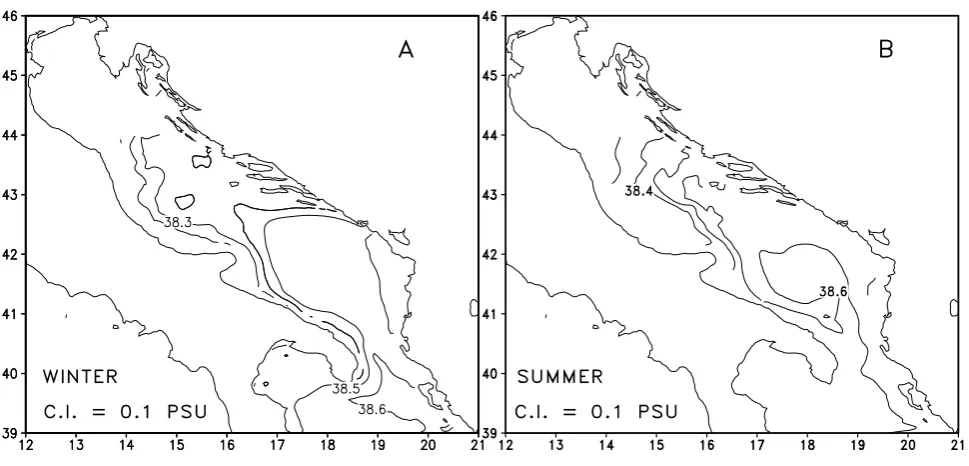
Fig. 7. Adriatic Intermediate Model (AIM). Seasonal surface salinity fields. (A): winter, (B): summer. Contour interval is 0.1 psu. Seasons definition as in Artegiani et al. (1997a, b).
Fig. 8. Adriatic Intermediate Model (AIM). Seasonal velocity trajectories at 75 m depth computed as if the flow were steady for 10 days. (A): winter, (B): summer. Not all the grid points have been plotted. Seasons definition as in Artegiani et al. (1997a, b).
the OGCM that seems to produce systematically higher sur-face temperatures with respect to the AIM, that makes use of the solar radiation penetration.
The salinity seasonal surface fields (Fig. 7) also indicate that the model is correctly representing the surface features observable in the seasonal climatologies. In both winter (Fig. 7a) and summer (Fig. 7b) the rivers’ freshwater dis-charge along the western coast of the northern Adriatic and
[image:11.595.57.539.349.579.2]gradi-Fig. 9. Adriatic Intermediate Model (AIM). Seasonal temperature fields at 75 m depth. (A): winter, (B): summer. Contour interval is 0.5◦. Seasons definition as in Artegiani et al. (1997a, b).
Fig. 10. Adriatic Intermediate Model (AIM). Seasonal salinity fields at 75 m depth. (A): winter, (B): summer. Contour interval is 0.1 psu. Seasons definition as in Artegiani et al. (1997a, b).
ent weakens in the northern Adriatic. This is a well-known feature of the Adriatic Sea phenomenology (Artegiani et al., 1997b). The summer freshening of the whole northern Adri-atic occurs despite the fact that during that season river dis-charge is at minimum, but the generalized wind weakening all over the basin (Fig. 2b) allows for an enhanced offshore spreading of the Po River fresh water discharge that affects the whole sub-basin and not only the western coastal regions.
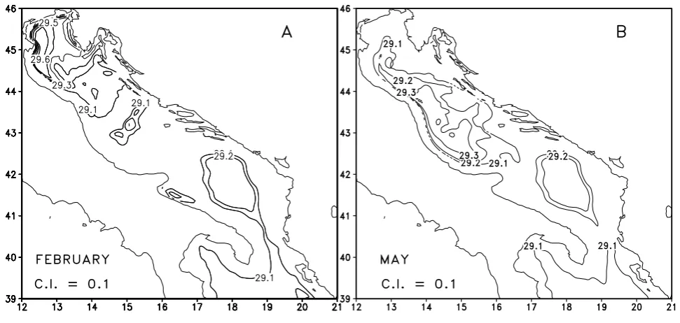
[image:12.595.56.541.350.583.2]per-Fig. 11. Adriatic Intermediate Model (AIM). Bottomσθdistribution. (A): February, (B): May. Contour interval is 0.1 kg/m3. For clarity,σθ
values lower than 29.1 kg/m3have been masked out.
Fig. 12. Adriatic Intermediate Model (AIM). σθ distribution in
February along the zonal section A of Fig. 1. Contour interval is 0.05 kg/m3.
sists, while the outflow appears to be largely recirculating into the SAd gyre. In the central Adriatic, the winter MAd gyre (Fig. 8a) appears very weak and disconnected from the southern Adriatic circulation, while in summer the two gyres (MAd and SAd) are connected by both the northward cur-rent on the eastern side and the southward curcur-rent on the western side of the basin. This pattern is in relative agree-ment with the dynamic height computations of Artegiani et al. (1997b) that indicate a stronger interconnection between the two gyres in summer-autumn rather than in winter. Inter-estingly, during winter the cyclonic circulation in the central
Adriatic is connected with a southward flowing vein of water originating from the north that almost disappears in summer. The analysis of the corresponding temperature and salinity fields indicates (see below) that this current is caused by the southward spreading of the dense water mass formed in win-ter over the northern Adriatic shelf.
The 75 m depth temperature and salinity fields for winter and summer are shown in Figs. 9 and 10, respectively. It can be noted that the winter vein of water coming from the north and interacting with the MAd gyre is characterized by tem-perature values lower than 12.0◦(Fig. 9a) and by salinity val-ues lower than 38.2 psu (Fig. 10a). These are valval-ues in good agreement with the definition of the northern Adriatic dense water mass given by Artegiani et al. (1997a). Therefore, it appears that the AIM is correctly representing the dense wa-ter formation in the northern Adriatic. We shall return lawa-ter to this feature by illustrating the distribution of bottomσθ. The
other notable feature appearing in the temperature and salin-ity distribution is the higher temperature and salinsalin-ity signa-ture of the inflow from the Otranto Strait and its entrainment into the southern Adriatic cyclonic circulation.
As stated above, the model seems to represent correctly the winter dense water formation over the northern Adriatic shelf. A confirmation of this comes from the examination of the bottomσθ distribution in February and May, as shown in
Fig. 11. In February (Fig. 12a), bottom water withσθ
[image:13.595.54.540.66.297.2] [image:13.595.50.286.360.537.2]south-Fig. 13. Adriatic Intermediate Model (AIM). Seasonally averaged meridional velocity sections in the Strait of Otranto (zonal section B of Fig. 1). (A): winter, (B): summer. Contour interval is 1 cm/s. Positive values denote northward flow. Seasons definition as in Artegiani et al. (1997a, b).
Table 4. Estimates of the southward transport (Sv) in the Otranto Channel from Gacic et al. (1999) and from the AIM simulation
Southward transport in Winter Summer the Otranto Strait (Sv)
Gacic et al. (1999) 1.40 0.71
AIM 1.36 1.27
ward displacement. Dense water having a lower σθ value
(29.2 kg/m3) is also located in the Pomo depressions. In May (Fig. 11b), no dense water can be observed over the northern Adriatic shelf and the dense water mass is now located in the middle Adriatic, where the Pomo depressions are now filled with water havingσθ values higher than 29.3 kg/m3. The
plot relative to the month of May is also indicating displace-ment along the bottom of the dense water mass toward the deep southern Adriatic. We can, therefore, conclude that the AIM is successfully representing the dense water formation process in the northern Adriatic, as well as its spreading into the middle Adriatic and the associated bottom water renewal in the Pomo Depressions, as described by Franco and Bre-gant (1980).
In the southern Adriatic the model is also reproducing the convective process leading to dense water formation. The Februaryσθ distribution along the zonal section A of Fig. 1
J F M A M J J A S O N D 4
6 8 10 12 14 16 18 20 22
(a)
deg C
AIM NASM
J F M A M J J A S O N D 35.5
35.75 36 36.25 36.5 36.75 37 37.25 37.5
(b)
psu
Fig. 14. Annual cycle of the basin averaged NASM temperature and salinity compared with the average computed over the AIM model domain sector corresponding to the NASM domain. Solid line: AIM, dashed line: NASM. (a): Temperature; (b): Salinity. Units are◦C for temperature and psu for salinity.
[image:14.595.310.547.397.584.2] [image:14.595.81.256.436.499.2]Fig. 15. Northern Adriatic Shelf Model (NASM) 2 m depth seasonal (winter and summer) circulation com-pared with the corresponding AIM sim-ulation. (A): AIM winter, (B): NASM winter, (C): AIM summer, (D): NASM summer. Units are m/s. Not all grid points are plotted. Seasons definition as in Artegiani et al. (1997a).
between 29.0 and 29.1 kg/m3. The breaking of the vertical stratification in the upper layers occurs in February, persists (weakly) in March, and in April the water column appears again to be density stratified. However, theσθ values
simu-lated by the model appear lower than the values reported by Ovchinnikov et al. (1987) for a dense water formation event in the southern Adriatic.
We end our analysis of the AIM results by showing, in Fig. 13, seasonally averaged sections of the meridional ve-locity in the Strait of Otranto (along zonal section B of
Fig. 16. Northern Adriatic Shelf Model (NASM) 2 m depth September circulation compared with the corresponding AIM simulation. (A): AIM, (B): NASM. Units are m/s. Not all grid points are plotted.
along with the corresponding estimates arising from the AIM simulation. It can be noted that the winter value is in good agreement with the Gacic et al. (1999) estimate, while the summer value appears larger than the corresponding estimate based on the observations.
3.2 Northern Adriatic Shelf Model (NASM)
We describe now the model simulations of the Northern Adriatic circulation obtained with NASM, in terms of basin averaged temperature and salinity annual cycle and of sur-face property distribution, compared with the corresponding AIM simulations. A comparison between the basin averaged NASM temperature and salinity and the corresponding AIM sector of the model domain is shown in Fig. 14. It can be seen that the temperature annual cycles simulated by the two models are in tight agreement (Fig. 14a). The salinity annual cycles (Fig. 14b), on the contrary, shows only a qualitative agreement, since the general trends are comparable, but the NASM basin averaged salinity appears systematically lower than the AIM averages. A possible explanation of this differ-ence is given below in terms of the differdiffer-ences in the circula-tion patterns simulated by the two models.
sim-Fig. 17. Northern Adriatic Shelf Model (NASM) surface temperature distribu-tion compared with the corresponding AIM simulation. (A): AIM winter, (B): NASM winter, (C): AIM summer, (D): NASM summer. Contour interval is 0.5◦C. Seasons definition as in Arte-giani et al. (1997a).
ulation, appears, also in this season, narrower than in the AIM. The occurrence of a southward current along the east-ern northeast-ern Adriatic coast (named Istrian Coastal Counter-current, ICCC) in summer has been recently described by Supic et al. (2000) by means of in situ current measurements and dynamic height computation. The circulation pattern that they describe for the summer occurrence of the ICCC resem-bles closely the NASM simulation results and, to a lesser ex-tent, AIM circulation features. It has to be stressed, however, that the seasonal averages shown in Fig. 15 are smoothing out rather strongly the circulation features produced by the two models. In fact, the monthly averages of the surface circu-lation field relative to September (Fig. 16) show that in both AIM and NASM, the ICCC emerges as part of a completely closed anticyclonic gyre. The gyre is smaller and less spa-tially extended in the AIM simulation (Fig. 16a) than that in the corresponding NASM field (Fig. 16b). It might be then that NASM, with a better horizontal resolution, is
produc-ing an element of the northern Adriatic summer circulation that AIM cannot capture. This is a point that obviously will deserve a close analysis in the planned future simulation ex-periments.
The AIM September circulation field (Fig. 16a) also ac-counts for the summer variability of the WACC path, a fea-ture that does not appear clearly in Fig. 5b due to the smooth-ing arissmooth-ing from the seasonal average. It can be noted that in September the WACC partially detaches from the coast, strongly meanders and forms (in agreement with observa-tion) southward of the Po River delta, both cyclonic and an-ticyclonic eddies.
[image:17.595.52.329.65.490.2]Fig. 18. Northern Adriatic Shelf Model (NASM) surface salinity distri-bution compared with the correspond-ing AIM simulation. (A): AIM win-ter, (B): NASM winwin-ter, (C): AIM sum-mer, (D): NASM summer. Contour interval is 0.5 psu for salinity values
<35.0 psu and 0.2 psu for salinity val-ues>35.0 psu. Seasons definition as in Artegiani et al. (1997a).
having the minimum temperatures in good agreement with the observations of Artegiani et al. (1997b). In summer the NASM surface (Fig. 17d) temperature is again in very good agreement with the corresponding AIM field and with the climatological observations.
Comparison of the NASM and AIM salinity fields con-firms the close similarities between the two models in win-ter (Fig. 18a and b). NASM is, however, resolving betwin-ter the fresh water contribution of the rivers discharging along the northern coast, since the individual river plumes can be noted both in summer and winter. From winter to summer the generalized freshening of the basin is reproduced by NASM (Fig. 18d) in a different fashion than from AIM (Fig. 18c), both in terms salinity values (NASM surface salinities are fresher) and in terms of horizontal distribution. Part of this difference can be explained in terms of the differences in the circulation patterns described above, since the NASM occur-rence of the ICCC prevents the inflow along the eastern coast of saltier water, that in AIM is advected northward. The
NASM development of the ICCC prevents this contribution and determines the lower surface salinities.
4 Conclusions
due to differences in the treatment of the short-wave radia-tion component of the heat flux in the two models. On the contrary, the AIM to NASM nesting allowed for a “clean” downscaling of the AIM circulation features on the NASM open boundary.
The AIM simulated circulation features are consistent with the known characteristics of the Adriatic Sea circulation, with the only difference being the reduced seasonal vari-ability of the WACC. However, the model has correctly re-produced the overall cyclonic circulation, the seasonal cy-cle of the scalar properties, and the dense water formation in the northern and southern Adriatic and the Otranto strait exchanges. Simulations with NASM showed, for the winter season, a strong degree of similarity with AIM. We can say that the finer NASM resolution and the effectiveness of the AIM coupling allowed for a simulation of the WACC north-ern Adriatic segment of superior quality with respect to AIM. This also applies to the simulation of the fresh water con-tribution from the Adriatic rivers. However, we have also described a strong difference between AIM and NASM in terms of surface circulation. NASM developed during sum-mer a feature comparable with the “Istrian Coastal Counter-current” that is only weakly appearing in the AIM simula-tions. The occurrence of this feature generates consistent differences between the AIM and NASM surface tempera-ture and salinity fields. This is interpreted in terms of a better skill of NASM (due to its finer resolution) to capture features of the northern Adriatic coastal circulation.
Acknowledgements. This research has been undertaken in the framework of the EU funded Mediterranean Forecasting System Pi-lot Project, MFSPP (contract MAS3-CT97-0171). We thank the two reviewers for their helpful and constructive criticisms.
The Editor in Chief thanks B. Cushman-Roisin and another ref-eree for their help in evaluating this paper.
References
Artegiani, A., Azzolini, R., and Salusti, E.: On the dense water in the Adriatic Sea, Oceanol. Acta, 12, 151–160, 1989.
Artegiani, A., Bregant, D., Paschini, E., Pinardi, N., Raicich, F., and Russo, A.: The Adriatic Sea general circulation. Part I: Air Sea interactions and water mass structure, J. Phys. Oceanogr., 27, 1492–1514, 1997a.
Artegiani, A., Bregant, D., Paschini, E., Pinardi, N., Raicich, F., and Russo, A.: The Adriatic Sea general circulation. Part II: Baro-clinic circulation structure., J. Phys. Oceanogr., 27, 1515–1532, 1997b.
Bignami, F., Marullo, S., Santoleri, R., and Schiano, M. E.: Long-wave radiation budget in the Mediterranean Sea., J. Geophys. Res., 100, 2501–2514, 1995.
Blumberg, A. F. and Mellor, G. L.: A description of a three-dimensional coastal ocean circulation model. In: Three-dimensional coastal ocean models, (Ed) Heaps, N. S., AGU, 1– 16, 1987.
Brankart, J. M. and Pinardi, N.: Abrupt cooling of the Mediter-ranean Levantine Intermediate Water at the beginning of the 1980’s: Observational evidence and model simulation, J. Phys. Oceanogr., 31, 2307–2320, 2001.
Castellari, S., Pinardi, N., and Leaman, K.: A model study of air-sea interactions in the Mediterranean Sea, J. Mar. Sys., 18, 89–114, 1998.
Cavaleri, L., Lavagnini, A., and Martorelli, S.: The wind climatol-ogy of the Adriatic Sea deduced from coastal stations, Nuovo Cimento, 19, 37–50, 1996.
Cavaleri, L. and Bertotti, L.: In search of the correct wind and wave fields in a minor basin, Mon. Weather Rev., 125, 1964–1975, 1997.
Da Silva, A. M., Young, C. C., and Levitus, S.: Atlas of surface marine data. NOAA Atlas NESDIS, 7, pp. 78, 1995.
Demirov, E. and Pinardi, N.: Simulation of the Mediterranean Sea circulation from 1979 to 1993: Part I. The interannual variability, J. Mar. Sys., 33/34, 23–50, 2002.
Flather, R. A.: A tidal model of the northwest European continental shelf, M´em. Soc. R. Sci. Li`ege, 6(X), 141–164, 1976.
Franco, P.: Oceanography of the northern Adriatic Sea: II. Hydro-logic features: cruises January–February and April–May 1966, Archo. Oceanogr. Limnol., Suppl., 17, 1–97, 1972.
Franco, P. and Bregant, D.: Ingressione invernale di acque dense nord Adriatiche nella fossa di Pomo, Atti IV Congr. Assoc. Ital. Oceanogr. Limnol., 1–10, 1980.
Gacic, M., Civitarese, G., and Ursella, L.: Spatial and seasonal vari-ability of water and biogeochemical fluxes in the Adriatic Sea. In: The Eastern Mediterranean as la laboratory basin for the assess-ment of contrasting ecosystems, (Eds) Malanotte-Rizzoli, P. and Eremeev, V. N., Kluwer Acad. Publ., 335–357, 1999.
Galperin, B., Kantha, L. H., Hassid, S., and Rosati, A.: A quasi-equilibrium turbulent energy model for geophysical flows., J. At-mos. Sci., 45, 55–62, 1988.
Gibson, J. K., Kallberg, P. K., Uppala, S., Hernandez, A., No-mura, A., and Serrano, E.: ERA description. ECMWF Re-analysis Project Report Series, 1, pp. 72, 1997.
Hellerman, S. and Rosenstein, M.: Normal monthly wind stress over the world ocean with error estimates, J. Phys. Oceanogr., 13, 1093–1104, 1983.
Jerlov, N. G.: Marine Optics, Elsevier Science, pp. 231, 1976. Killworth, P. D.: Deep convection in the world ocean, Rev.
Geo-phys. Space Phys., 21, 1–26, 1983.
Killworth, P. D.: Time interpolation of forcing fields in ocean mod-els, J. Phys. Oceanogr., 26, 136–143, 1996.
Kondo, J.: Air-sea bulk transfer coefficients in diabatic conditions, Boundary Layer Meteorol., 9, 91–112, 1975.
Korres, G. and Lascaratos, A.: A one way nested eddy resolving model of the Aegean and Levantine basins: Implementation and climatological runs, Ann. Geophysicae, this issue, 2003. Kovacevic, V., Gacic, M., and Poulain, P. M.: Eulerian current
mea-surements in the Strait of Otranto and in the southern Adriatic, J. Mar. Sys., 20, 255–278, 1999.
Legates, D. R. and Wilmott, C. J.: Mean seasonal and spatial vari-ability in a gauge corrected global precipitation, Int. J. Climatol., 10, 121–127, 1990.
Maggiore, A., Zavatarelli, M., Angelucci, M. G., and Pinardi, N.: Surface heat and water fluxes in the Adriatic Sea: Seasonal and interannual variability, Phys. Chem. Earth, 23, 561–567, 1998. Malanotte Rizzoli, P.: The northern Adriatic Sea as a prototype of
convection and water mass formation on the continental shelf. In: Deep convection and deep water formation in the Oceans, (Eds) Chu, P. C. and Gascard, J. P., Elsevier Oceanography Series, 57, 229–239, 1991.
the Ionian Sea in the period 1997–1999, J. Mar. Sys., 33/34, 133– 154, 2001.
Marchesiello, P., Mc Williams, J. C., and Shchepetkin, A.: Open boundary conditions for long-term integration of regional oceanic models, Ocean Modelling, 3, 1–20, 2001.
Mellor, G. L.: An equation of state for numerical models of oceans and estuaries, J. Atmos. Oceanic Technol., 8, 609–611. 1991. Mellor, G. L.: User’s guide for a three-dimensional primitive
equa-tion, numerical ocean model, AOS Program Report, Princeton University, Princeton NJ, 34, 1998.
Mellor, G. L. and Blumberg, G.: Modeling vertical and horizontal diffusivities with a sigma coordinate system, Mon. Weather Rev., 113, 1279–1383, 1986.
Mellor, G. L. and Yamada, T.: Development of a turbulence closure submodel for geophysical fluid problems, Rev. Geophys. Space Phys., 20, 851–875, 1982.
Oberh¨uber, J. M.: The budgets of heat, buoyancy and turbulent ki-netic energy at the surface of the global ocean. An atlas based on the COADS data set, Max Planck Inst. f¨ur Meteorologie Report, 15, pp. 20, 1988.
Oey, L. Y.: Eddy energetics in the Faroe-Shetland channel: a model resolution study, Cont. Shelf Res., 17, 1929–1944, 1998. Oey, L. Y. and Chen, P.: A nested-grid ocean model: with
applica-tion to the formaapplica-tion of meanders and eddies in the Norwegian Coastal Current, J. Geophys. Res., 97, 20 063–20 086, 1992. Ovchinnikov, I. M., Zats, V. I., Krivosheya, V. G., Nemirosky, M. S.
and Udodov, A. I.: Winter Convection in the Adriatic and forma-tion of deep eastern Mediterranean waters, Ann. Geophysicae, 5B, 89–92, 1987.
Payne, R. E.: Albedo of the sea surface, J. Atmos. Sci., 29, 959– 970, 1972.
Pinardi, N., Allen, J. I., Demirov, E., De Mey, P., Korres, G., Las-caratos, A., Le Traon, P. Y., Maillard, C., Manzella, G., and Tzi-avos, C.: The Mediterranean ocean Forecasting System: First phase of implementation (1998–2001), Ann. Geophysicae, this issue, 2003.
Poulain, P. M.: Adriatic Sea surface circulation as derived from drifter data between 1990 and 1999, J. Mar. Sys., 29, 3–32, 2001. Poulain, P. M. and Cushman-Roisin, B.: Circulation. In: Physical Oceanography of the Adriatic Sea. Past, present and future, (Eds) Cushman-Roisin, B., Gacic, M., Poulain, P. M., and Artegiani, A., Kluwer Academic Publ., 67–109, 2001.
Provini, A., Crosa, G., and Marchetti, R.: Nutrient export from the Po and Adige river basin over the last 20 years, Sci. Total Env., suppl., 291–313, 1992.
Pullen, J. D.: Modeling studies of the coastal circulation off
north-ern California, Ph. D. Dissertation in Oceanography, Oregon State Univ., 145, 2000.
Pullen, J. D. and Allen, J. S.: Modeling studies of the coastal circu-lation off northern California: Shelf response to a major Eel river flood event, Cont. Shelf Res., 20, 2213–2238, 2000.
Pullen, J. D. and Allen, J. S.: Modeling studies of the coastal circu-lation off northern California: Statistics and patterns of winter-time flows, J. Geophys. Res., 106, 26 959–26 984, 2001. Raicich, F.: Note on flow rates of the Adriatic rivers. Istituto
Talas-sografico Sperimentale Trieste, Technical Report, RF02/94, pp. 8, 1994.
Raicich, F.: On the fresh water balance of the Adriatic Sea, J. Mar. Sys., 9, 305–319, 1996.
Reed, R. K.: An evaluation of formulas for estimating clear sky insolation over the ocean, NOAA-ERL 352-PMEL Techn. Rep., 26, pp. 25, 1975.
Reed, R. K.: On estimating insolation over the ocean, J. Phys. Oceanogr., 7, 482–485, 1977.
Reynolds, R. W. and Smith, T. M.: Improved global sea surface temperature analyses using optimum interpolation, J. Climate, 7, 929–948, 1994.
Rosati, A. and Miyakoda, K.: A general circulation model for upper ocean simulation, J. Phys. Oceanogr., 18, 1601–1626, 1988. Sannino, G. M., Bargagli, A., and Artale, V.: Numerical Modeling
of the mean exchange through the Strait of Gibraltar, J. Geophys. Res., 107(CB) Ant. No. 3094, 2002.
Smagorinsky, J.: Some historical remarks on the use of nonlinear viscosities. In: Large eddy simulations of complex engineering and geophysical flows, (Eds) Galperin, B. and Orszag, S., Cam-bridge Univ. Press, 1993.
Smolarkiewicz, P. K.: A fully multidimensional positive definite ad-vection transport algorithm with small implicit diffusion, J. Com-put. Phys., 54, 325–362, 1984.
Smolarkiewicz, P. K. and Clark, T. L.: The multidimensional posi-tive definite advection transport algorithm: further development and applications, J. Comput. Phys., 67, 396–438, 1986. Supic, N., Orlic, M., and Degobbis, D.: Istrian coastal
countercur-rent and its year to year variability, Est. Coast. Shelf Sci., 51, 385–397, 2000.
Vogt, J. A.: Adriatic Sea surface temperature: Satellite and drifter observations between May and October 1995. M. S. Thesis, Naval Postgraduate School Monterey, pp. 85, 2002.