Annales Geophysicae (2003) 21: 2201–2218 cEuropean Geosciences Union 2003
Annales
Geophysicae
A theoretical model for double diffusive phenomena in cloudy
convection
P.-A. Bois1and A. Kubicki1,2
1Laboratoire de M´ecanique de Lille, UMR CNRS 8107, U.F.R de Math´ematiques, Bˆat. M3, U.S.T.L., F-59655 Villeneuve
d’Ascq, France
1,2now at: The Service d’A´eronomie, UMR CNRS 7620, Tour 25, 4 Place Jussieu , F-75252 Paris Cedex, France
Received: 24 October 2001 – Revised: 10 April 2003 – Accepted: 17 April 2003
Abstract. Using classical rheological principles, a model is proposed to depict the molecular diffusion in a moist-saturated dissipative atmosphere: due to the saturation con-dition existing between water vapor and liquid water in the medium, the equations are those of a double diffusive phe-nomenon with Dufour effect. The double diffusivity is im-portant because of the huge diffusivity difference between the liquid phase and the gaseous phase. Reduced equa-tions are constructed and are then applied to describe the lin-ear free convection of a thin cloudy layer bounded by two free surfaces. The problem is solved with respect to two destabilizing parameters, a Rayleigh numberRaand a moist
Rayleigh numberRh. Two instabilities may occur: (i)
os-cillatory modes, which exist for sufficiently large values of the Rayleigh number: these modes generalize the static in-stability of the medium; (ii) stationary modes, which mainly occur when the moist Rayleigh number is negative. These modes are due to the molecular diffusion, and exist even when the medium is statically stable: the corresponding mo-tions describe, in the moist-saturated air, configuramo-tions such as “fleecy clouds”. Growth rates are determined at the in-stability threshold for the two modes of inin-stability occurring in the process. The case of vanishing moisture concentra-tion is considered: the oscillatory unstable case appears as a singular perturbation (due to the moisture) of the station-ary unstable state of the Rayleigh-B´enard convection in pure fluid, and, more generally, as the dynamical perturbation of the static instability. The convective behaviour of a cloud in the air at rest is then examined: the instability of the cloud is mainly due to moisture, while the instability of the surround-ing air is mainly due to heatsurround-ing.
Key words. Atmospheric composition and structure (cloud physics and chemistry) – Meteorology and atmospheric dy-namics (convective processes, mesoscale meteorology)
Correspondence to: P.-A. Bois ([email protected])
1 Introduction
The role of the moisture on the dynamics of atmospheric air has been studied several years ago, from various points of view. For instance, Dudis (1972), Einaudi and Lalas (1973), Durran and Klemp (1982a, b; 1983), considered its influence on the Brunt-V¨ais¨al¨a frequency and inviscid flows (such as mountain lee waves). Einaudi and Lalas and later, Durran and Klemp, focused their attention on media with a non-constant distribution of moisture with respect to the altitude. Deardorff (1976, 1980), and Betts (1982) constructed re-duced schemes using the so-called “liquid-water moist po-tential temperature”: such schemes were used by Bougeault (1981a, b), in order to study the moist atmospheric turbu-lence. From another point of view, Kuo (1961, 1965), Ogura (1963) studied convective instability in dissipative media. More recently, Bretherton and Smolarkiewicz (1987, 1988, 1989) considered the motion, the appearance and the disap-pearance of clouds under moist convection effects. Some consequences of the diffusion taking into account the mi-crostructure of the medium have also been exhibited by Kambe and Takaki (1975), and Merceret (1977). In these works, the double diffusive characteristics of the medium are either absent (when dissipation is neglected in the medium), or not really taken into account.
binary Fick’s law is chosen for the diffusion of the total wa-ter in the total mixture{air + total water}(e.g. in Bretherton’s papers); (ii) a binary Fick’s law is chosen for the diffusion of water vapor in the gaseous phase, i.e.{water vapor + dry air}, the diffusion of the liquid water being neglected: this law (see Hijikata and Mori, 1973) is also adopted in works deal-ing with industrial thermodynamics, and a variant may be found in Deardorff’s papers and Bougeault’s papers. Hence, the first question set in the present paper is that of the choice of a law of molecular diffusion: by applying the basic princi-ples of thermodynamics and of rheology, we construct a dif-fusion law stating precisely the validity of Bougeault’s for-mulae. A simplified form of this law is also discussed in the case of weak moisture.
Another singularity arises in the analysis of the phe-nomenon of moist convection. Since the water concentration, sayqv, is small, the Schmidt numberS∗, characterizing the
molecular diffusion, plays an effective role in the equations through the combination 1/S = qv/S∗ only; this number
is very small whenS∗ is of order unity (in practice, in this mixture,S∗ ≈ 0.721). However, the factor 1/S multiplies a laplacian, so that even for small 1/S, the molecular diffu-sion acts through some boundary layers, and, in a stability problem, such boundary layers may originate specific insta-bilities.
The following paper is organized as follows: in Sect. 2, the equations of motion are set up using a classical mixture theory; the basic equations are written using a model of con-tinuous medium, with the diffusive dissipation being given using the principles of thermodynamics. The major simpli-fying assumption is that the condensed water is treated as an aerosol (its pressure is neglected in the whole mixture, so that we are led to describe it as a polytropic gas whose adiabatic constant is zero); the additional assumption of neg-ligible diffusion of the liquid water is not needed. A second basic assumption is that of a saturated medium. These as-sumptions are classical in non-precipitating cloud theories. Because the molecular diffusion in saturated mixtures is not very well known, the molecular diffusion law is especially examined. It is shown that the phenomenon follows a gener-alized Fick’s law with Dufour effect. In fact, the problem of ternary convection may be finally reduced to a convection in a binary mixture, and this reduced problem is that of a dif-fusion with Dufour effect. However, some properties of the ternary nature of the mixture remain present in the model, as will be seen later.
In the Sect. 3, the linearized gravity wave equation gov-erning the motions is derived. The study is made using the asymptotic frame of the Boussinesq approximation already used in previous papers (Bois, 1991, 1994). The use of this approximation first implies the existence of a particular so-lution describing a static state of the medium, depicted with the help of unique variable (the altitude referred to the “dry” atmospheric scale). Second, the characteristic vertical scale of the perturbation motion is small before the atmospheric scale, and the characteristic time of the motion is also scaled with the help of static data (namelyt0=c0/g, wherec0
de-notes the speed of sound in the medium at the rest); this for-mulation follows the classical analysis of Spiegel and Vero-nis (1960). An advantage of using the asymptotic formu-lation of the Boussinesq approximation is to allow one to write the equations with the help of two scales (the fast scale, which is the scale of the convection, and the scale of the strat-ification of the medium, or slow scale); their ratio is the small Boussinesq parameter, sayε. After linearizing the equations around the static state, we obtain a wave equation general-izing to the considered medium the classical gravity wave equation used, for instance, in the Rayleigh-B´enard convec-tion. The analogy with the equations of thermohaline con-vection is also noted.
In Sect. 4, we consider shallow convection in the medium at rest. Since the considered problems are dissipative, two diffusion factors remain present in the reduced problem. In order to solve the singular perturbation occurring in the phe-nomenon, we first assume that the Schmidt number S∗ is small, of the same order asqv. We introduce the reduced
Schmidt number S, which is, itself, of order unity. Af-ter solving the corresponding instability problem (so-called auxiliary problem) it is simpler to obtain the solution of the real problem by examining the behaviour of the solution of the auxiliary problem whenSgoes to infinity. By applying this procedure, a moist Rayleigh-B´enard problem is solved, and its solution is described with respect to two destabilizing parameters, namely the Rayleigh number Ra, and a moist
Rayleigh number Rh, itself proportional to the total water
gradient. Finally, the following properties are derived: first, because of the permanent exchange of mass between the two liquid phases, a stationary instability mainly occurs for a neg-ative moist Rayleigh number, even whenRais, itself,
nega-tive. The corresponding cloud configurations appear in a first approximation, as motions of the dry air and the aerosol only. These motions describe fleecy cloud configurations. Such motions are partially located in the statically stable region of the (Ra, Rh) plane, in the same manner as the salt
fin-gers found in thermohaline convection (see Baines and Gill, 1969). Second, an oscillatory instability appears in an angu-lar region of the (Ra,Rh) plane, itself located between the
P.-A. Bois and A. Kubicki: Double diffusive phenomena in cloudy convection 2203 determination allows one to select the preferential
instabili-ties occurring in the medium. To end with, we match the in-stability conditions in the cloud with the corresponding con-ditions in unsaturated air (clear air), so that we may conclude about the instability of a cloud surrounded by clear air.
2 Rheological model
2.1 Thermodynamics of moist saturated air
The medium is modelled as a ternary mixture: dry air, wa-ter vapor and condensed wawa-ter. The constituents are identi-fied by the subscriptsg(dry air),v(water vapor),L(liquid water). The densities are denotedρg,ρv,ρL. The density
of the medium beingρ = ρg +ρv+ρL, the
concentra-tions are denoted by qα = ρα/ρ, and satisfy the relation
qg +qv +qL = 1. We will also use the total water
con-centrationqw = qv+qL (more generally, the subscriptw
will denote “total water”). The velocity of each constituent is denoted uα, and the barycentric velocity of the fluid is
u = qgug+qvuv+qLuL. The diffusion velocities vα are
then defined by va=uα−u, and satisfy the relation
ρgvg+ρvvv+ρLvl=0. (1)
The specific variables defining the system satisfy the ther-mostatic Gibbs-Duhem equation
de=T ds−pd(1/ρ)+gLdqL+gvdqv+ggdqg, (2)
wheree denotes the internal energy per mass unit, and the gα’s denote the free enthalpies per mass unit of the
con-stituents. For a reversible infinitesimal transformation of the medium, because of the saturation hypothesis, the free enthalpies gL and gv are equal. Hence, setting dqw =
dqL+dqvand usingdqg+dqw ≡0, Eq. (2) reads
de=T ds−pd(1/ρ)−(gg−gv)dqw. (3)
After Eq. (3) we have e = e(s, ρ, qw), T =
(∂e/∂s)(s, ρ, qw)andp= −(∂e/∂υ)(s, ρ, qw), whereυ=
1/ρ. Eliminatings between these relations, we have in the saturated mixture
e=e(T , ρ, qw), p=p(T , ρ, qw). (4)
In the sequel we assume that the mixture is an ideal mixture of polytropic gases. Moreover, following a classical approx-imation for the aerosols, we neglect the pressure of the liquid phase so that this phase is also a polytropic gas (with a zero polytropic constant).
2.2 The Clausius-Clapeyron equation
The saturation equation is the Clausius-Clapeyron equation. We introduce the latent heat of vaporization of the liquid, namelyLv = hv−hL, (hα is the specific enthalpy of the
phase α). A form of this equation, valid when the liquid
phase is an aerosol (see, for instance, Zemansky, 1968), may be written as
dpv=LvρvdT /T . (5)
It is of interest to examine some consequences of the Clausius-Clapeyron formula, when the partial pressure of the liquid phase is neglected. The dry air, the water vapor and the whole mixture follow the equations of state, respectively, pg=RgρgT , pv=RvρvT ,
p=RmρT , Rm=Rgqg+Rvqv, (6)
whereRg andRv are two constants. The third relation (6)
expresses Dalton’s law. As said above, the partial pressure pL is neglected in Dalton’s law. Let us now differentiate
Dalton’s law. After some calculation and using the Clausius-Clapeyron equation, we obtain the relation
dqw =dqL+dqv=
−qg qv
dqv−
Rm
Rg
dp p +
Rm
Rg
Lv
RvT2
dT . (7)
The relation (7) expresses the total water variations with re-spect to the variations of vapor, pressure and temperature. Now, denotingcp v andcp L the heat capacities of the wa-ter vapor and the liquid wawa-ter, respectively, the latent heat of vaporization can be written as
Lv=Lv0+ cp v−cp L
(T −20) , (8)
Lv0 and20being two constants. Lv0 is the latent heat at
the temperature 20. Introducing Eq. (8) in the
Clausius-Clapeyron equation (written with the variablesqv,ρandT),
we obtain the relations qv=q0
ρ020β
ρTβ exp
{30+β−1}
1−20
T
,
3= L0
Rv20
, β=1−cp v−cp L
Rv
, (9)
where q0, ρ0,20 are some constants. By eliminatingρ in
(9) with the help of the third of (6), we deduce, after some calculation, the relations
qv/qg=Qs(p, T )=
Rgps0G(T )
Rv[p−ps0G(T )]
,
ps0=q0Rvρ020,
G(T )=(20/T )β−1exp[{30+β−1}(1−20/T )]. (10)
Sinceqv/qgdenotes the concentration of water vapor in the
gaseous phase, the pressureps0G(T )is the saturation
pres-sure of the water vapor for the corresponding vapor con-centration, with the constantps0being the saturation
pres-sure of the water vapor at the temperature20. The function
Qs(p, T )defined in Eqs. (10) is the saturation concentration
(10) may be taken as “equations of state” and used in order to eliminate secondary variables in the equations of motion. Ex-tractingqv/qgas functions ofp, ρ, andT from Eqs. (10) and
the third of (6), an explicit expression of the equation of state p=p(qv, ρ, T )could be obtained by inserting these
expres-sions in Dalton’s law. However, although these expresexpres-sions theoretically could allow one to eliminate some unknowns in the equations of motion, it is simpler to keep the original variables in these equations.
2.3 The diffusion equations
We now consider a moving system. The barycentric mo-tion of the system is described using the material derivative d/dt = ∂/∂t +u·∇. First, consider the balance of mass
for the dry air: this equation, (so-called molecular diffusion equation) reads
ρdqg
dt +∇·(ρgvg)=0. (11)
The balance of mass for the whole mixture in the barycentric motion reads
∂ρ
∂t +∇·(ρu)=0. (12)
The diffusion velocities are themselves related to the gradi-ents of concentrations by Fick’s law. For the mixture consid-ered here, this Fick’s law (see Appendix A) reads
ρgvg =C
∇qv−
qv
qg ∇qg
, (13)
where C is a positive constant coefficient. Because qv is
small, an approximation of Eq. (13) isρgvg =C∇qv; such
equation has been used in Kubicki and Bois (2000). How-ever, it will be seen later that, in convection problems, as we further investigate, this approximation is too rough if we look for a realistic solution. Hence, even for smallqv, we
will keep the whole relation (13) in what follows. The rela-tion (13) inserted in Eq. (11) provides the new equarela-tion ρdqg
dt +C∇·
∇qv−
qv
qg ∇qg
=0. (14)
Now consider the first law of thermodynamics: for a moving mixture of dissipative fluids, this law, written in terms of en-thalpy in place of the internal energy, after some calculation, provides the equation
cp
dT dt −
1 ρ
dp dt +hL
dqL
dt +hv dqv
dt +hg dqg
dt =
8+k ρ1T −
1
ρ{∇·(ρqLhLvL+ρqvhvvv+ρqghgvg)}.(15) The coefficientcp denotes the heat capacity of the mixture
with constant pressure and concentrations. On the right-hand side, the dissipation is the sum of the viscous dissipation8, the thermal dissipationk1T /ρ (kis the thermal conductiv-ity), and the diffusive dissipation in the third term: thehα’s
are the partial enthalpies of the constituents.
According with classical hypothesis of small diffusion velocities (Bowen, 1976), the thermodynamical potentials e, h, gare related to the partial potentialseα, hα, gα by the
approximate relations e = Pq
αeα, h = Pqαhα, g =
Pq
αgα. Note that(∂h/∂qα)p,T =hα.
Finally, using Eq. (5) and Eq. (14), we replace dqg by
−(dqv+dqL), andhv−hLbyLv: the Eq. (15) reads, after
some rearrangement, cp
dT dt −
1 ρ
dp dt +Lv
dqv
dt = k
ρ1T −qqvg·∇(hg−hv)+
Lv
C ρ∇·
∇qv−
qv
qg ∇qg
+8. (16)
The motion of the medium is described by using the classical variables u, p, ρ, T ,and two concentrations, sayqvandqg.
It is convenient to write the diffusion equations with the same variables: hence, replacingdqgby−(dqv+dqL)in Eq. (14)
and using Eq. (7) to eliminatedqL, Eq. (14) also reads
−qq qv
dqv
dt +
Rm
Rg
Lv
RvT2
dT dt −
Rm
Rg
1 p
dp dt =
C
ρ∇·
∇qv−
qv
qg ∇qq
. (17)
The two Eqs. (16) and (17) are two symmetrical forms of the diffusion equations: assuming thatdp/dtis known in these equations (it is an approximate consequence of the Boussi-nesq equations, see Sect. 3) the real unknowns, in Eqs. (16) and (17), are dT /dt and dqv/dt. These equations can be
solved in two independent forms dealing with linear com-binations of these quantities. The molecular diffusion and the heat conduction appear in laplacians figuring in the right-hand sides of these equations and cannot separately be con-sidered; this property characterizes a double diffusive phe-nomenon.
Finally, the equations of motion for a saturated mixture are: the third Eq. (6), and Eqs. (9), (12), (16), (17), to which we must add the balance of momentum
ρdu
dt +∇p=ρg+µ0
1u+1 3∇(∇·u)
, (18)
where µ0 denotes the dynamic viscosity. Finally, we have
a complete set of 8 scalar equations for the 8 unknowns u, p, ρ, T , qv, qg.
3 The Boussinesq equations
3.1 Validity conditions and nondimensional equations The Boussinesq approximation refers to the motion to a static state of the medium, in which the variables depend only on one variable, namely the altitude scaled by the so-called at-mospheric heightH = p0/(ρ0g), wherep0andρ0denote
P.-A. Bois and A. Kubicki: Double diffusive phenomena in cloudy convection 2205 The general validity conditions of the Boussinesq
approx-imation (Bois, 1991) first imply that the characteristic scale Lof the motion is small before H : L/H = ε 1, and second, that the characteristic velocity scaleU of the mo-tion is related to εby the equalityU√ρ0/p0 = ε: that is
equivalent to choosing a characteristic time of the motion t0=H
√
ρ0/p0. We don’t discuss the validity of these
con-ditions, which are assumed to be true. We note, however, that, when rewritten for the significant nondimensional pa-rameters of the problem (defined further, see relations (25), F =U/√gLis the Froude number of the flow), these con-ditions imply the relations
ε1, F2=ε. (19)
The variables are now scaled by characteristic values: U, L, ρ0, 20, cp g. The scaling pressure isp0 = ρ0cp g20,
and we haveRg =(γ−1)cp g/γ,γ being the adiabatic
con-stant of the dry air. Rewritten with nondimensional variables the former equations read
ρdu dt +
1 ε2∇p+
1 ερk=
1 Re
1u+1
3∇(∇·u)
, (20)
−qg qv
dqv
dt +
qq+
Rv Rg qv 3v T2 dT dt − 1 p dp dt = 1 ReS∗
1
ρ∇·(∇qv− qv
qg
∇qg), (21)
Cp dT dt − 1 ρ dp dt +
γ −1 γ Rv Rg 3v dqv dt = 1 PrRe
1 ρ1T +
χv−1
ReS∗
1
ρ∇qv·∇T+
γ −1 γ
Rv
Rg
3v
ReS∗
1 ρ∇·
∇qv−
qv
qg ∇qg
+ ε
2
Re
8, (22)
qv=q0
1 ρTβexp
{30+β−1}
1− 1 T
, (23)
p=γ −1 γ
qg+
Rv
Rg
qv
ρT . (24)
The Eq. (12) remains unchanged. We have set in the Eqs. (20)–(24)
Re=
LUρ0
µ0
, Pr =
µ0cp0
k,
S∗= µ0
C , F =
U √
gL
ε= U
p cp020
, χv=
cp v
cp g,
χL=
cp L
cp g, 3v= Lv
Rv20
, (25)
30andβbeing defined in Eqs. (9) and (10). The two
diffu-sion parameters are the Prandtl numberPr and the Schmidt
numberS∗, which match the thermal dissipation (Prandtl) and the molecular dissipation (Schmidt) with the viscous dis-sipation (Reynolds numberRe). We have used the relation
(8) and the relations
cp=qgcp g+qvcp v+qLcp L,
Cp=qg+χvqv+χLqL,
3v=30+(1−β)(T −1). (26)
The first two equations of (26) are valid for polytropic gases, the third equation results from Eq. (8). Since we are con-cerned only with shallow convection, it is possible to find equilibrium solutions to the system Eqs. (20)–(24). Hence, we consider an equilibrium state (u = 0), having a pre-scribed temperature distribution and a prepre-scribed water va-por concentration, say T = T0(ζ ), qv = Qv0(ζ ), then
Eqs. (20)–(24) are satisfied (up to and including orderε)by pressure, density and dry air concentrationsp=P0(ζ ), ρ0=
R0(ζ ), qg = Qg0(ζ ): denoting with primes the derivatives
d/dζ, these quantities satisfy the static equations
P00(ζ )+R0(ζ )=0, ζ =εz,
P0(ζ )=
γ −1
γ (Qg0(ζ )+(Rv/Rg)Qv0(ζ )R0(ζ )T0(ζ ),(27)
Q0w0(ζ )= −Qg0(ζ )
Q0v0(ζ ) Qv0(ζ )
+ γ
(γ −1)T0(ζ ) +
(Qg0(ζ )+(Rv/Rg)Qv0(ζ ))
3
0+β−1
T0(ζ )
+1−β T0
0(ζ )
T0(ζ )
.(28) The variable z is the physical vertical variable (say z0) scaled byL, while ζ (= εz)is the same variable z0 scaled byH. Note that Eq. (28) is nothing but the static form of the Eq. (7).
3.2 Boussinesq asymptotic expansion
Following the Boussinesq procedure (Bois 1991), we now expand the variables with respect toεin the following form: p=P0(ζ )+ε2ρ,˜ ρ=R0(ζ )+ερ,˜
T =T0(ζ )+εT ,˜ qv=Qv0(ζ )+εq˜v,
qg =Qg0(ζ )+εq˜g, u= ˜u. (29)
We expand Eqs.(12) and (20)–(24) with respect toε. Dis-carding the static terms, we obtain the following perturbation equations
∇·u˜=O(ε), (30)
R0(ζ )
du˜
dt +∇p˜+ ˜ρk= 1 Re
−Qg0(ζ ) Qv0(ζ )
dq˜v
dt +
Qg0(ζ )+
Rv
Rg
Qv0(ζ )
λ0(ζ )
T0(ζ )
dT˜ dt
− ˜w
Q
g0(ζ )
Qv0(ζ )
Q00v(ζ )−
Qg0(ζ )+
Rv
Rg
Qv0(ζ )
λ0(ζ )
T00(ζ ) T0(ζ )
−P 0 0(ζ )
P0(ζ )
=
1 ReS∗
1 R0(ζ )
1q˜v−
Qv0(ζ )
Qg0(ζ )
1q˜g
+O(ε), (32)
Cp0(ζ )
dT˜ dt +
γ −1 γ
Rv
Rg
λ0(ζ )
dq˜v
dt +
w γ −1
γ
Rv
Rg
λ0(ζ )Q0v0(ζ )+Cp0(ζ )T00(ζ )−
P00(ζ ) P0(ζ )
= 1
PrRe
1 R0(ζ )
1T˜ +γ −1 γ
Rv
Rg
λ0(ζ )
ReS∗
1 R0(ζ )
1q˜v−
Qv0(ζ )
Qg0(ζ )
1q˜g
+O(ε), (33)
˜ qv
Qv0(ζ ) + ρ˜
R0(ζ ) −
3
0+β−1
T0(ζ ) −β
T˜
T0(ζ )
=O(ε),(34)
Rgq˜g+Rvq˜v
RgQg0(ζ )+RvQv0(ζ )
+ ρ˜ R0(ζ )
+ ˜ T
T0(ζ )
=O(ε). (35)
We have set in Eqs. (32)–(35) λ0(ζ )=
30+(1−β)(T0(ζ )−1)
T0(ζ )
,
Cp0(ζ )=Qg0(ζ )+χvQv0(ζ )+χLQL0(ζ ). (36)
Simplified forms of Eqs. (30)–(35) may be looked at in two ways: (i) by assuming that the water concentration is weak (see below) and, (ii) by approximating the values of the coef-ficients by their values at a given level (shallow convection, see Sect. 4).
3.3 The reduced problem
In order to look for simplifying assumptions about the sys-tem (30)–(35), we first note that the magnitude of both wa-ter vapor concentration and liquid wawa-ter concentration are usually small, of the same order: their order of magnitude (namely the parameterq0 introduced in Eqs. (9) and (23))
is, in practice, about 10−3. Hence, we expand the system with respect toq0: keeping only the leading terms of the
ex-pansion, many coefficients in Eqs. (30)–(35) take simpler ap-proximate forms. However, this simplification induces some singularities. The most important of these is that the double diffusive character of the system disappears when we neglect terms of orderq0(the laplacians 1q˜v and1q˜g figuring in
Eqs. (32) and (33) become negligible) . In order to avoid this
singularity, we now assume thatS∗is also small, of the same orderq0as the water concentrations. Thus, we set
S∗=q0S, (37)
where S is a modified Schmidt number, which is itself as-sumed of order unity. Since the Schmidt number appears only in the combination (1/S∗)1q˜v, the assumption S =
O(1)allows one to keep the laplacian in the simplified equa-tions, and, further, when we letS go to infinity in the solu-tions of realistic problems, we can directly examine the in-fluence of the singular perturbation induced by the double diffusivity whenS∗=O(1).
For smallq0, taking into account the assumption (37), the
Eqs. (32) and (33) read dT˜
dt + ˜w
T00(ζ )+1
= 1
PrRe
1 R0(ζ )
1T˜+
γ −1 γ
Rv
Rg
λ0(ζ )T0(ζ )
ReS∗R0)(ζ )
1q˜v−Qv0(ζ )1q˜g+O(ε), (38)
− 1
Qv(ζ )0
dq˜v
dt + λ0(ζ )
T0(ζ )
dT˜ dt −
˜ w
1
Qv0(ζ )
Q0v0(ζ )−
λ0(ζ )
T00(ζ ) T0(ζ )
−P 0 0(ζ )
P0(ζ )
=
1 ReS∗R0(ζ )
1q˜v−Qv0(ζ )1q˜g+O(ε). (39)
In Eqs. (38) and (39) we have approximated the variables by constant values when their expansions for smallq0don’t lead
to singularities: for instance, for smallq0,Cp0andCg0are
approximated by 1. The system [(30), (31), (34), (35), (38), (39)] may be yet simplified by extracting the unknownq˜g(or,
equivalently, the unknownq˜v) from the algebraic Eq. (35), as
a linear combination of the other variables. The remaining system is the reduced system associated with the problem. Note that, since we have allowed in the system the coeffi-cients depending on the variableζ, the equations are valid for deep convection, as well as for shallow convection.
4 Moist Rayleigh-B´enard shallow convection 4.1 Linearized equation
The preceding equations are now applied to the study of shal-low free convection in a thin layer (a cloud). The levelz=0 is the mean altitude of the convecting cloud. The thickness of the layer is chosen as scaling lengthLin the equations. Because of the weak thickness of the layer, and since we are interested only in terms of order 0 with respect toε, all slowly varying coefficients of the Eqs. (31)–(36) and (39)–(40) are approximated by their values atz=0, namely
−P00(0)=R0(0)=T0(0)=1,
P.-A. Bois and A. Kubicki: Double diffusive phenomena in cloudy convection 2207 Qv0(0)=q0, Qg0(0)=1−q0Rv/Rg,
30v(ζ )=30, Cp0(0)=1. (40)
Taking into account the assumption of smallq0, we set ˜
qv=q0q˜˜v, q˜L=q0q˜˜L,
˜
qg=q0q˜˜g, Q
0
v0=q0Q
0
0. (41)
The state of rest (namelyu˜ =0,ρ˜= ˜p= ˜T = ˜˜qv=0)is an exact solution of the reduced system (30)-(31)-(34)-(35)-(38)-(39). The linearized equations associated with the sys-tem, approximated by their first term with respect toq0, then
read
∇·u˜ =0 (42)
∂u˜
∂t +∇p˜+ ˜ρk= 1 Re
1u,˜ (43)
˜
ρ+(1−30)T˜ + ˜˜qv=0, (44)
˜
ρ+ ˜T = −q0
h ˜˜
qg+(Rv/Rg)q˜˜v
i
. (45)
∂q˜˜v
∂t +0w˜ =
30µ−1
ReS
h
1q˜˜v−q01q˜˜g
i + 30
PrRe
1T ,˜ (46)
∂T˜ ∂t +N
2w˜ = 1
PrRe
1T˜ + µ ReS
h
1q˜˜v−q01q˜˜g
i
. (47) We have used, in the preceding equations, the notations 0=Q00− γ
γ −1 +30, N
2=T0 0+1,
µ= γ −1 γ
Rv
Rv30. (48)
Becauseq˜˜g figures in Eqs. (43)–(47) only through the com-binationq0q˜˜g, the limit of Eqs. (43)–(47) for vanishingq0is
singular (8 equations for seven unknowns only). Because all boundary conditions are zero in a free convection problem, this singularity may be avoided by assuming that the vari-ablesu,˜ p,˜ ρ,˜ T ,˜ q˜˜v are themselves of orderq0, whileq˜˜g is
of order 1. Hence, we set ˜
ρ=q0ρ∗, q˜˜v=q0qv∗,
˜˜
qg =qg∗, T˜ =q0T∗,
˜
p=q0p∗, u˜=q0u˜∗. (49)
The first approximation of Eq. (45) now takes the nondegen-erate form
ρ∗+T∗= −qg∗. (50)
Hence, after Eq. (44) we also have
qg∗=qv∗−30T∗. (51)
Finally, extractingqv∗from Eq. (51), the system (42)–(47) reduces to the following
∇·u∗=0,
∂u∗ ∂t +∇p
∗+
ρ∗k= 1 Re
1u∗,
ρ∗+T∗+qg∗=0, (52)
∂qg∗
∂t +
0−30N2
w∗= − 30 ReS
1T∗,
∂T∗ ∂t +N
2w∗= 1 Re
3
0µ
S +
1 Pr
1T∗. (53)
The system (52)–(53) clearly exhibits the particularities of the problem: first, the problem is a double diffusive problem for a fictitious binary mixture whose equation of state is the third equation listed in Eq. (52). Second, due to the form of the right-hand side of the first equation listed in Eq. (53), the diffusion equations in this medium involve the Dufour effect (the time derivative∂qg∗/∂t doesn’t depend on1qg∗but on 1T∗only !). The significance of the first diffusion Eq. (53) may be understood by the help of the static Eq. (28): effec-tively, taking into account the shallow convection assump-tion and the smallness ofq0, the leading approximation of
this equation reads
Q0w0= −Q00+30+30T00+
γ γ −1 = −
0−30N2
,(54)
so that0−30N2is nothing but the total water gradient in
the medium at rest. Since Q0w0 is of order q0, a rigorous
study would impose to cancel0−30N2(at the order 0 with
respect toq0) in the system (52)–(53). In fact, it is equivalent
to solve this system for arbitrary values of0−30N2and,
furthermore, to consider small values of this parameter; this procedure is adopted in the sequel.
4.2 Solution of the linear Rayleigh-B´enard problem with two free surfaces
The Rayleigh-B´enard problem with free surfaces is the sim-plest case of boundary conditions associated with the system (52)–(53). In spite of its academic character, it allows one to simply exhibit analytical solutions (in fact, with the help of the only dispersion equation). The linear stability of the sys-tem may be studied by a normal modes analysis, by looking for solutions in the form u∗=U(x, y, z)eηt, withη=ξ+iω. Since we don’t envisage boundary conditions depending on the horizontal variables, all modes are assumed in the form: (u∗, v∗, w∗, p∗, ρ∗, T∗, qg∗)
W, to an equation of sixth order with constant coefficients. This equation itself takes a simpler form, by introducing the characteristic parameters
Ra= −PrR2eN 2,
Rh=PrRe2
0−30N2
= −PrReQ0w0, τ =S/Pr.(56)
Rais the Rayleigh number,Rhis the moist Rayleigh number,
τ is the ratio of the diffusivities of the medium. Moreover, we adopt the notations
σ =ηRe, K2=k2+h2,
D2=d2/dz2−K2, D2n=(D2)n. (57) Rewritten with these notations, the equation satisfied by Wreads
σ Pr(30µ+τ )D6W−σ2Pr(30µ+τ+τ Pr)D4W
+hσ3τ Pr2+K2{(30µ+τ )Rh−30Ra}
i D2W
= −σ τ PrK2(Ra−Rh)W. (58)
The boundary conditions are free surfaces conditions at z=0 andz=1. If we require continuity of the temperature and the concentration at the boundaries, the other boundary conditions are standard (see Drazin and Reid, 1981), so that we assume
W =D2W =0, T =0,
Q=0, in z=0 and z=1. (59)
The boundary conditions (59) are satisfied by particular so-lutions of (58) of the formW = W sinnπ z, n ≥ 1, where W=const. The dispersion equation takes the algebraic form σ Pr(30µ+τ )Q6+σ2Pr(30µ+τ +τ Pr)Q4
+hσ3τ Pr2+K2{(30µ+τ )Rh−30Ra}
i Q2
−σ τ PrK2(Ra−Rh)=0, (60)
where we have set
Q2=K2+n2π2, Q2n=(Q2)n. (61) Equation (60) is a third-degree equation with respect toσ, similar (but, however, simpler) to the equation from Baines and Gill (1969) for thermohaline convection. The thresholds are reached forRe(σ ) =0, so that these thresholds are as-sociated with stationary solutions or purely oscillatory solu-tions of Eq. (60): the procedure is standard (see Drazin and Reid, 1981) and leads to the following conclusions: (i) sta-tionary solutions: Eq. (58) possesses stasta-tionary solutions if the condition
(10µ+τ )Rh−30Ra=0, (62)
is satisfied independently ofn; this property characterizes a singular bifurcation, because all harmonics of a solution ap-pear at the same threshold as the fundamental mode. Hence, the growth rates of the unstable solutions must effectively be computed in order to select the mode which effectively ap-pears in an unstable process (see Sect. 4.3); (ii) oscillatory solutions: two conditions must be satisfied: first, denoting the pulsation of the solution(σ =i), exists only if the inequality
τ{30(µ−1)+τ+τ Pr}Ra−τ2PrRh
(30µ+τ )(30µ+τ +τ Pr)
≥ 27π 4
4 , (63)
is satisfied. Second, in the half plane defined by the condi-tion (63),2is, itself, positive, only if
(30µ+τ )Rh−30Ra≥0, (64)
is satisfied. In the (Ra, Rh) plane, both inequalities are
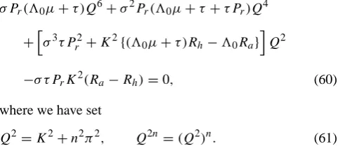
[image:8.595.47.288.502.610.2]simultaneously satisfied inside the angular sectorU AY of Fig. 1. Ais the polycritical point of the problem. The for-mulae (62) and (63) allow one to determine the coordinates (Ra a, Rha)ofA, namely
Ra a= 27π 4
4
(30µ+τ )2
τ[30(µ−1)+τ]
,
Rha =27π 4
4
30(30µ+τ )
τ[30(µ−1)+τ]
. (65)
Since the left-hand side of Eq. (54) is of orderq0, we see
that the only realistic values of the numberRh/(PrRe2)are
small of the same order. Hence, the solutions exhibited here are available only in the region of the(Ra, Rh)plane, such
as Rh/(PrR2e) = O(q0) 1. Note that this condition is
not very restricting, because, in general, the Reynolds num-ber is large. The above analysis also shows that the least value ofRh in an oscillatory unstable state is that reached
at the polycritical pointA. Hence, in order to satisfy the conditionRh/(PrR2e)1, it is of interest to study the
pos-sible positions of Awhen the intensity q0 of the moisture
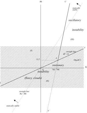
(even remaining small) varies. We have plotted, in Fig. 2, the way followed byAin the(Ra, Rh)plane whenτ varies
from 0 to+ ∞. Eliminatingτ between the two formulae (65), the equation of this curve may be easily derived, namely Rha = {(µ+1)Ra a−[(µ−1)2Ra a2+27π4µRa a]1/2}/(2µ).
For infiniteτ, Ais located at the pointC =27π4/4(≈657) of theRa-axis: this point is just the threshold of the stationary
instability in a pure fluid. For smaller values, and, in particu-lar, for vanishingτ, the trajectory is asymptote to the straight line of equationRa a=µRha+27π4µ/[4(µ−1)]. Hence, for vanishingq0(large values ofτ),Ais located near theRa
-axis, and for large values ofq0(small values ofτ),Ais far
from theRa-axis. However, the inequalityRh/(PrRe2))1
P.-A. Bois and A. Kubicki: Double diffusive phenomena in cloudy convection 2209
Ra Y
stationary instability
( fleecy clouds)
O ( q0Re2 )
(II)
A
statically stable
statically stable
oscillatory
instability
O 785 790 13,7
straight line
Ra = Rh
(III)
V
(I)
Rh U
X
straight line
[image:9.595.147.449.64.456.2]Ω2 = 0
Fig. 1. Linear instability diagram of moist-saturated air in the (Ra, Rh) plane. In order to exhibit the different regions more explicitly, the
scales are not respected in this figure. The realistic instability is located in the shaded regionRh =O(q0R2e), so that the polycritical point
may be either inside or outside the instability domain. The straight lineRa=Rhdelineates the statically stable region. The numerical values
chosen for determine the polycritical pointAare (units M.K.S.A.):L0= 2600 103J/kg,20=288◦K,cp v =1004 J/(kg.◦K),Rv=464
J/(kg.◦K),Rg=287 J/(kg.◦K),S=S∗/q0=721,Pr =0,76,q0=10−3.
practical problems, because the pointAis located in a real-istic region of the(Ra, Rh)plane, oscillatory instability may
also exist.
4.3 Stable and unstable regions and growth rates at the in-stability thresholds
The preceding analysis, although allowing one to determine the instability thresholds, doesn’t place in evidence the sta-ble and the unstasta-ble regions of the(Ra, Rh)plane. In order
to localize these stable and unstable regions, because of the indetermination led by the equality (62), it is convenient to examine the real part ofσin the neighbourhood of the thresh-olds:
(i) Stationary threshold XA: as a preliminary remark, we note that a procedure followed by Baines and Gill
(1969) may be applied here: setting σ =Q2θ , R0a=K2Ra/Q6, Rh0 =K
2R
h/Q6,(66)
Eq. (60) takes the canonical form τ Pr2θ3+Pr(30µ+τ+τ Pr)θ2
+[(30µ+τ )Pr−τ Pr(R0a−R
0
h]θ
+(30µ+τ )R0h−30R0a=0. (67)
C
150
100
50
0
600 657 739 1000 1200 1400 1600 1800 2000
Figure 2
[image:10.595.50.285.63.203.2]Ra D Rh
Fig. 2. Locus of the pointAin the (Ra, Rh) plane whenτvaries
from 0 to +∞. The numerical values are the same as in Fig. 1. The way followed byAwhenτvaries (continuous curve) is almost rectilinear. This curve goes very slowly to its asymptote (dotted straight line).
is satisfied, this equation possesses one real positive root only. Hence, the half plane defined by Eq. (68) is an un-stable region with unun-stable direct modes: one mode ex-actly for a given value of(R0a, Rh0), i.e. for fixedRa, Rh,
andK. In order to determine the growth rates and the wavelengths of those unstable modes (and the most un-stable modes themselves), we linearize Eq. (67) near the threshold defined by Eq. (68): hence, we set
Rh0 =R0h0+1R0h, R0a=Ra00, θ=0+1θ , (69) whereRh00andRa00satisfy the relation
(30µ+τ )Rh00−30Ra00, (70)
and where1Rh0 and1θ are assumed small. After lin-earizing Eq. (67), and taking into account the relation (69), we obtain the following relation between1Rh0 and 1θ
1θ= 30(30µ+τ )1R 0
h
Pr
τ[30(µ−1)+τ]R0h0−30(30µ+τ )
.(71)
After the second equation listed in (65), becauseRh0<
Rha along the half-straight lineXA, the denominator of Eq. (71) is negative alongXA. Hence, for negative 1Rh0, 1θ is real and positive: the stable region is lo-cated overXA, and the unstable region is located under XA(Fig. 1). Moreover, Eq. (71) allows one to find the most unstable mode in the following manner: first, we deduce from Eq. (71) by reinserting the variablesσ and Rhwith the help of Eq. (66)
1σ =Qn2
30(30µ+τ )(K2/Qn6)1Rh
Pr
τ[30(µ−1)+τ](K2/Qn6)Rh0−30(30µ+τ )
. (72)
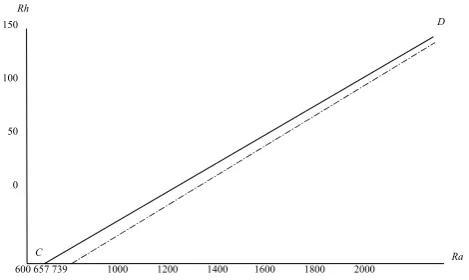
By studying the variations of 1σ with respect to n, withKbeing fixed, we deduce from Eq. (72) (see Ap-pendix B) that the greatest value of1σis obtained when n = 1; hence, the most unstable mode is always the fundamental mode. Furthermore, restricting the study to the casen = 1, we deduce, after some calculation, the wave numberKmaxfor which the maximum of1σ,
say1σmax, is reached: Kmaxis the only root of the
al-gebraic equation (Kmax2+π2)3
Kmax2
1− π 2
Kmax2
!
= −τ[30(µ−1)+τ]Rh0 30(30µ+τ )
(73)
(the calculations are given in the Appendix B). The cor-responding1σmaxis given by the formula (72). Kmax
is a function of Rh0 (or, equivalently Ra0); hence, it
varies along the whole straight lineXA, up toA. For instance, for the numerical values used in Fig. 1, the curvesKmax =F (Ra0)and|1σmax/1Rh| =G(Ra0)
are drawn on Fig. 3, where Fig. 3a shows thatKmaxis
al-ways greater than the valueπ/ √
2(≈2.221)of the wave number of a regular B´enard convection.Kmaxdecreases
whenRa0increases, until the value is reached at the
crit-ical value ofRa0. Figure 3b shows that the growth rate
of the fundamental mode is much larger than the first harmonic (n = 2), and that, forn ≥ 3, these growth rates become negligible. Of course the formula (72) be-comes invalid in the neighbourhood of the critical point: near this point we must use a second order expansion, which leads to an expression of1σmaxproportional to
(1Rh)1/2(see later).
(ii) Oscillatory thresholdAU. Since the instability near the thresholdAU is a regular problem, the instability al-ways occurs for the fundamental moden =1, and the corresponding wave numberKc=π/
√
2: this situation is analogous to that of the classical Rayleigh-B´enard convection. However, the preceding analysis is useful in order to determine the growth rates of the oscillating unstable modes; we set
Ra0 =R0a0+1Ra0, R0h=Rh00, (74) where (Ra00,Rh00) are the coordinates of a point ofAU, and1Ra0 denotes a small variation ofRa0 from an arbi-trary valueRa00. We set, moreover,
θ=iφ0+1θ, (75)
whereφ0is real, and we assume that1θis small. Since
iφ0is an exact imaginary root of Eq. (67),R0a0andR 0
h0
satisfy the relations
τ{30(µ−1)+τ +τ Pr}R0a0−τ 2P
P.-A. Bois and A. Kubicki: Double diffusive phenomena in cloudy convection 2211 =(30µ+τ )(30µ+τ+τ Pr), (76)
φ02=
1 τ Pr
30µ+τ−τ (R0a0−R 0
h0)
= (30µ
+τ )Rh00−30Ra00
Pr(30µ+τ +τ Pr)
. (77)
Now, linearizing Eq. (67) for the unknown1θ and us-ing Eq. (76) and the first of (77), we obtain after some calculation
1θ=1ψ+i1φ, (78)
1ψ= τ[30(µ−1)+τ+τ Pr]1R 0
a
2
(30µ+τ+τ Pr)2+τ2Pr2φ02
,
1φ=
τ2Pr2φ02+30(30µ+τ +τ Pr1Ra0
2φ0Pr
(30µ+τ+τ Pr)2+τ2Pr2φ02
. (79)
After Eq. (79), for positive 1Ra0, 1ψ is always posi-tive along the thresholdAU. In fact,1ψis nothing but some scaling of the real growth rateRe(1σ ); hence, us-ing Eq. (66) to reintroduce the variablesσ, Ra, Rh, K,
and noticing that, for the oscillatory instability,K2 = Kc2=π2/2, we obtain
Re(1σ )=(3/2)π21ψ=
τ[30(µ−1)+τ+τ Pr]
9π2
(30µ+τ +τ Pr)2+τ2Pr2φ021Ra
. (80)
We have drawn on Fig. 4, for the same numerical val-ues as in the preceding figures, the curve|1σ/1Ra| =
F (Ra0)along the half straight lineU A. Note thatφ02
can be extracted, in terms ofRa0, from the relations
(77). In the same manner as in Fig. 3, the neighbour-hood of the critical point is singular, but, after Eq. (79), only the phase becomes singular at this point.
(iii) Neighbourhood of the critical point. Near the critical point, the linear expansion of the dispersion equation is invalid, for the stationary case, as well as for the oscil-latory case. SinceRe(1σ )is small in this neighbour-hood, we now set
Ra0 =Ra a0 +1Ra0, R0h=Rha0 +1Rh0,
θ=1ψ+i1φ, (81)
where1R0a, 1R0h, 1ψ, 1φare assumed small. Since the critical point is a stationary threshold and an oscil-latory threshold simultaneously, the following relations (30µ+τ )Rha0 −30Ra a0 =0,
10
8
6
4
2
Ra0
Kmax
0 790 12665
n = 1
n = 2
n = 3
Kmax = 2,22 =π/v2
Kmax = 4,44 = 2π/v2
π
2π
3π
(a)
Ra0
103×∆σ
max/∆Rh
n = 1
n = 2
33,3
n = 3
8,3
3,7
0 790 12665
invalid linear expansion
(b)
Figure 3
Fig. 3. Wave numberKmax(a) and growth rates (b) of the three
first stationary unstable modes. The numerical values are the same as in Fig. 1 (the scales are not respected on the figure forRa0). The
x-axis is taken along the stationary threshold, the variable being the Rayleigh numberRa0. The figure is invalid in the vicinity of
the asymptotes and, in particular,Ra a(shaded region), because the linearized formula (71) becomes invalid. It is also invalid when
Ra > Ra a, because this region is already unstable. WhenRa0→ −∞,|1σ/1Rh| →0 very slowly (as|Ra0|−1/2).
(30µ+τ )−τ (R0a a−Rh0
a)=0,
τ{30(µ−1)+τ+τ Pr}R0a a−τ2PrR0ha
=(30µ+τ )(30µ+τ+τ Pr), (82)
are satisfied. We first rewrite Eq. (67) by separating its real part and its imaginary part, taking into account the relations (82). Hence, we obtain the two following real equations
τ Pr21ψ3−3τ Pr21ψ 1φ2+
Pr(10µ+τ +τ Pr)(1ψ2−1φ2)
−τ Pr(1R0a−1R
0
h)1ψ+
(10µ+τ )1Rh0 −301Ra0 =0, (83)
1φ n
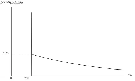
[image:11.595.311.542.61.358.2]5,73
Ra0 103×Re
(∆σ)/∆Ra
0 790
[image:12.595.51.288.64.206.2]Figure 4
Fig. 4. Growth rate of the oscillatory most unstable mode. Thex -axis is taken along the oscillatory threshold, the variable being the moist Rayleigh numberRh0. The numerical values are the same as
in Fig. 1. WhenRa0→ ∞,Re(1σ )/1Rh→0 asRa0−1.
2(30µ+τ+τ Pr)1ψ+τ (1Rh0 −1R
0
a)
o
=0. (84) According to Eq. (84), we separately consider the cases 1φ=0 and1φ6=0. We obtain the following conclusions:
(a) if1φ 6= 0 : 1φ2may be extracted from Eq. (84) and inserted in Eq. (83). This equation is then an equa-tion of the third degree for the unknown1ψ. Since we look for solutions of Eq. (83) only for small1Rh0 and 1Ra0, approximated values of the roots can be looked for. We obtain one positive root if the condition τ Pr1R0h− [30(µ−1)+τ+τ Pr]1Ra0 is negative; this
condition corresponds to a point(R0a, Rh0)located be-yond the oscillatory thresholdV U of the(Ra0, Rh0)plane (see Fig. 1). In this half plane, the condition1φ2≥0 is satisfied if the inequality(10µ+τ )1Rh0−301Ra0 ≥0
is satisfied. Finally, the corresponding modes exist if the figurative point(Ra0, Rh0)is located in the oscillatory re-gion previously determined on Fig. 1. The values of 1ψ, 1φare
1ψ=τ[30(µ−1)+τ+τ Pr]1R 0
a−τ2Pr1Rh0
2(30µ+τ +τ Pr)2
+o(1Rh0, 1Ra0), (85)
τ Pr1φ2=
(30µ+τ )1R0h−301R0a
30µ+τ +τ Pr
+o(1R0h, 1R0a). (86)
(b) if1φ = 0 : 1ψ is directly given by Eq. (83), which possesses a solution only if the inequality (30µ +
τ )1Rh0 −101R0a≤0 is satisfied; this corresponds to a
figurative point inside the stationary unstable region of Fig. 1. In this case the solution reads
τ Pr1ψ2=
301Ra0 −(30µ+τ )1Rh0
30µ+τ+τ Pr
+o(1Rh0, 1Ra). (87)
After Eqs. (85) and (87), the order of magnitude of the growth rates is O(301Ra −(30µ + τ )1Rh)1/2 in the
stationary region, and 0(τ[30(µ−1)+τ +τ Pr]1Ra −
τ2Pr1Rh)in the oscillatory region. The three expansions
(85), (86) and (87) may be asymptotically matched without difficulty, either with Eq. (71) (for the stationary instabil-ity), or with Eq. (79) (for the oscillatory instability). The behaviour of the oscillations is given, in the latter case, by Eq. (86). Finally, in the(Ra, Rh) plane, the stable region
is the region inside the angular domainXAU (Fig. 1). The thresholdXAleads to direct instabilities (stationary onset). The thresholdAU leads to unstable oscillating modes (os-cillatory onset). The growth rates of these modes are those calculated above.
4.4 The fleecy configurations of clouds
It is of interest, in order to understand the role of the diffu-sion in the medium, to compare the instability regions in the (Ra, Rh)plane, to the static instability regions. In fact, it
is well-known (see Durran and Klemp, 1982a or Bois 1994) that the moist Brunt-V¨ais¨al¨a frequency of the medium, say Nm, is given by the formula
Nm2 =N2[1+O(q0)]−Qw0 0≈ −Ra[1+O(q0)]+Rh,(88)
so that the neutral line of static stability, in the (Ra, Rh)
plane, is (at orderq0) the straight lineRh =Ra(the dotted
line of Fig. 1). Hence, the stationary instability is partially lo-cated in the statically stable region (the angular sectorXOT of Fig. 1). In this region, the instability regime which sets in is entirely analogous to the well-known “salt fingers regime”, existing in the thermohaline convective instability (see Nield, 1967 or Huppert and Turner, 1981). Indeed, as said formerly, this regime is a very slow motion of dry air and liquid water only; effectively, the variablesq˜gandq˜Ldefined in Eq. (29)
are of orderq0, while the variableq˜v, (after Eq. 49) is of
or-derq02. Hence, rather than “moisture fingers”, the solution
depicts, in fact, the fleecy appearance of clouds in an air at the rest.
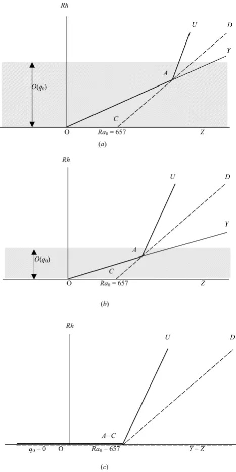
4.5 The caseS∗=O(1)
As we have seen above, the caseS∗=O(1)may be deduced from the preceding analysis by examining the behaviour of its solution whenS → ∞; in fact, this case corresponds to τ → ∞in the former formulae. Whenτ → ∞, the pointA of the(Ra, Rh)instability moves along the curveCDof this
plane, towardsC(see Fig. 2 and Fig. 5b). This point becomes exactly the point C when τ = +∞. Since the instability thresholds are delineated by straight lines joiningAandO itself, the corresponding positions of these thresholds may be very easily followed. More precisely, for infiniteτ the inequalities (63) and (64) become
Ra≥
Pr
1+Pr
Rh+
27π4
P.-A. Bois and A. Kubicki: Double diffusive phenomena in cloudy convection 2213 while the equality (62) now reads
Rh=0. (90)
After Eq. (90), at order 0 with respect toq0, the
station-ary instability threshold becomes theRa-axis itself: the
sta-ble region is the half planeRh > 0, the unstable region is
the half planeRh < 0. From Eq. (89), the oscillatory
un-stable region is the angleU CY of the(Ra, Rh)plane (see
Fig. 5c), whereC is the pointRa =Ra0 = 27π4/4 of the
Ra-axis. In fact, for vanishing moisture, i.e. q0 → 0, the
Ra-axis forRa > Ra0is not a singular bifurcation line. At
order 0 with respect toq0(Fig. 5c) the thickness of the
real-istic region of the flow is zero, so that this region reduces to theRa-axis itself; stationary instability is, in this case,
irrel-evant. On the contrary, oscillatory instability is realistic: the stable part of theRa-axis isRa < Ra0, the unstable part is
Ra > Ra0. Moreover, since the unstable region corresponds
to the boundary2 =0 of the “oscillatory” instability, this instability is, in fact, stationary. We recognize the instability scheme of the classical Rayleigh-B´enard convection, where the instability is due to the only Rayleigh number. This be-haviour is regular, since, for vanishingq0, the fluid becomes
a pure fluid. At order 1 with respect toq0(Fig. 5b), the
re-alistic region of the flow is a very narrow strip around the Ra-axis, and the critical pointAis distinct ofC. The case
τ → ∞also allows one to understand the singularity occur-ring if we directly assume{q01, S∗=O(1)}in Eqs. (20)
to (24): in this latter case Eq. (53) is replaced by ∂qg∗
∂t +
0−30N2
w∗=0, ∂qg∗
∂t +N
2w∗= 1 PrRe
1T∗ (91)
and the problem is now governed by the system [(52), (91)], which reduces to the equation
σ PrD6W−σ2Pr(1+Pr)D4W+
h
σ3Pr2+K2Rh
i
D2W = −σ PrK2(Ra−Rh)W. (92)
Let us look for stationary solutions of Eq. (92): such solu-tions (except the state of rest) exist only if Rh = 0, i.e if
0−30N2 = 0. The first equation (91) degenerates in this
case, so that the system (52)–(91) is now a system of 6 scalar equations for seven unknowns. However, we can note that, in this case, the changes of variables defined by (49) are su-perfluous. The original variablesu,˜ p,˜ ρ,˜ T˜ are solutions of the system (42), (43), and the two equations
˜
ρ+ ˜T =0, N2w˜ = 1 PrRe
1T .˜ (93)
The first equation listed in Eq. (93) is the leading approxima-tion of Eq. (45), and the second is the staapproxima-tionary version of the second equation in Eq. (91). Equations (42), (43), (93) constitute a complete, regular set foru,˜ p,˜ ρ,˜ T˜, which are solutions of an exact stationary Rayleigh-B´enard problem.
D
Y U
O Ra0 = 657 Z
Rh
C O(q0)
A
(a)
D
O Ra0 = 657 Z
O(q0)
A
Y U
Rh
(b)
D U
q0 = 0 O Ra0 = 657 Y = Z
A=C Rh
(c)
Figure 5
C
Fig. 5. Successive positions of the oscillatory instability threshold for decreasingq0. Whenq0 → 0 (and, hence, τ → +∞), the
thickness of the realistic region decreases so that, for vanishingq0,
the oscillatory instability region progressively goes to the stationary instability region of the classical Rayleigh-B´enard convection (in order to exhibit the different regions more explicitly, the scales are not respected on the figure).
Finally, in this case, a stationary solution of the full problem exists only ifRa ≥ 27π4/4, instead of the fullRa-axis, as
shown above. Contrary to the stationary solutions, the oscil-latory solutions are not singular in this case. Moreover, if we let the heat conductivity go to zero (i.e. forPr → ∞),
tak-ing into account the definitions (56), the oscillatory thresh-old defined by Eq. (89) becomes −N2 = −(0−30N2).
[image:13.595.311.545.64.531.2]the oscillating modes go to zero (for instance, after Eq. 57), so that these modes become stationary, and the condition 2 > 0 has no sense. The oscillatory instability threshold is, in this case, the whole straight lineU V of Fig. 1, i.e. ex-actly the static threshold. Hence, the oscillatory instability is the regular dynamical degeneracy of the static instability of the medium.
5 Convection in unsaturated air
Because a cloud is always confined between layers of clear air, it is of interest to match the results of the preceding anal-ysis with those of the corresponding analanal-ysis in unsaturated air: it is simple to repeat the analysis in this case. In such a medium, Eq. (3) remains valid, taking into account that, now,qv=qw. The diffusion Eq. (11) also remains valid, but
Eq. (16) is replaced by cp
dT dt −
1 ρ
dp dt =
k
ρ1T −qgvg·∇(hg−hv)+8. (94) The scaled form of the diffusion equations now read
dqv
dt = 1 ReS∗
1
ρ1qv, (95)
Cp
dT dt −
1 ρ
dp dt =
1 PrRe
1 ρ1T
+χv−1 ReS∗
1
ρ∇qv·∇T + ε2 Re
8. (96)
Since there is not a change of phase in the medium, the static Eq. (28) is replaced by the equation
Rv−Rg
Rg
Q0v0(ζ )= − γ (γ −1)T0(ζ )
−
Qg0(ζ )+
Rv
Rg
Qv0(ζ )
R00(ζ ) R0(ζ )
+T 0 0(ζ )
T0(ζ )
. (97) The Boussinesq analysis of the problem does not require one to use the parameterSinstead ofS∗. The reduced linearized Eqs. (42) and (43) remain valid, while Eqs. (45), (46), (47) are replaced by
˜
ρ+ ˜T = −q0
Rv−Rg
Rg q˜˜v, (98)
∂q˜˜v dt +Q
0 0w˜ =
1 ReS∗
1q˜˜v, (99)
∂T˜ ∂t +N
2w˜ = 1
PrRe
1T .˜ (100)
Equations (99) and (100) explicitly show the disappearance of double diffusivity when S∗ = Pr, the operator applied
toT˜ andq˜˜
v being, in this case, the same in both Eqs. (99)
and (100). The singularity of Eq. (98) is the same as that of Eq. (45), and may be similarly treated. Finally, defining the parameters
Ra= −PrRe2N2, R
00
h = −PrRe2Q
0 0,
τ∗=S∗/Pr, (101)
and looking for solutions in the form (55), we obtain forW the equation
D8W−σ (1+Pr+τ∗Pr)D6W
+σ2Pr(1+Pr+τ∗Pr)D4W+
n
−σ3Pr2τ∗
−K2(Rv−Rg)τ∗PrRh00/Rg+Ra
o D2W
=σ K2τ∗Pr
Ra+(Rv−Rg)Rh00/Rg
W. (102)
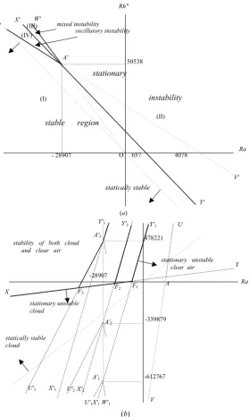
Equation (102) with boundary conditions (Eq. 59) may be discussed as follows: (i) stationary solutions: such solutions exist if the condition
Ra≥ −τ∗(Rv−Rg)Rh00/Rg+27π4/4, (103)
is satisfied. In the(Ra, Rh00)plane, the inequality (103)
de-fines a half plane bounded by the straight line X0Y0 (see Fig. 6a), with the unstable region mainly corresponding to positive values ofRaand positive values ofRh00; (ii)
oscil-latory solutions: denoting the pulsation (σ = i) two conditions must be satisfied: first,2being given, solutions exist only if the inequality
τ∗Pr
τ∗(1+Pr)Ra+(1+τ∗Pr)(Rv−Rg)Rh00/Rg
(1+τ∗)(1+P
r)(1+τ∗Pr)
≥ 27π 4
4 , (104)
is satisfied. Second, in the half plane defined by Eq. (104), 2is, itself, positive only if the inequality
RgRa+
τ∗(1+τ∗Pr)
1+Pr
(Rv−Rg)Rh00≤0, (105)
is satisfied. In the (Ra, Rh00) plane, both conditions (104)
and (105) are simultaneously satisfied inside the angular sec-torU0A0W0of Fig. 6. The pointA0, which also lies on the straight lineX0Y0, is the polycritical point. Figure 6 shows the behaviour of the system when the parametersS∗andPr
are almost equal (here: S∗ =0.72, Pr = 0.76). In Fig. 6a
the variables areRaandRh00The coordinates ofA0are very
large (A0is far from the origin), and the angleU0A0W0is very sharp. Moreover, 2 is small inside the domain U0A0W0. In Fig. 6b the variables are Ra and Rh (itself defined in
Eq. (56):Rhis a relevant variable if we consider a problem
[image:14.595.49.286.615.710.2]P.-A. Bois and A. Kubicki: Double diffusive phenomena in cloudy convection 2215
F1
F2
U
(b) U'1X'1 W'1
A
U'3 X'3
A'1
A'2
A'3
F3
Ra
-612767 -28907
X
Y stationary unstable clear air
stationary unstable cloud
stability of both cloud and clear air
V
-339879
Y'2
statically stable cloud
U'2 X'2
Y'3
Figure 6
478221
Y'1
O 657 4078 Ra 50538
mixed instability
Y' U'
A'
stable region
(III)
X'
(I) (IV)
stationary
instability
oscillatory instability
statically stable
V' Rh"
- 28907
(II)
(a)
[image:15.595.161.441.63.530.2]W'
Fig. 6. Instability diagram in clear air: (a)in the(Ra, Rh00)plane;(b)in the(Ra, Rh)plane. The numerical values are the same as in
Fig. 1. In Fig. 4a the stability parameterR00his defined with respect to the total moisture of the medium. Because the Schmidt number is very near the Prandlt number, the double diffusion is weak (almost absent) in this figure, the oscillatory instability being confined in a very sharp angular sectorU0A0W0. In Fig. 6b, the parameterRh= −Rh00+30Ra+PrRe2[30−γ /(γ−1)]is used instead ofRh00, in order to be able
to match together stable and unstable regions of both saturated and unsaturated cases, as it occurs in the coupled instability of two layers of fluid. In the latter case, three values ofReare considered: (i)Re=1 (stable region inside the angleXF1Y01); (ii)Re=150 (stable region
inside the angleXF2Y02); (iii)Re =300 (stable region inside the sectorXF3A03Y03): in that case, the instability of the clear air may be
oscillatory (thresholdF3A03).
surrounded by two layers of unsaturated air, the two stability diagrams of the clear air layers and of the cloud itself may be superimposed (Fig. 6b); the stability is confined in the region XF Y0 orXF A0Y0 of this figure, according to the values of the Reynolds number. The figure also shows that the instabil-ity of the cloud is mainly due to moisture, while the heating first destabilizes the surrounding air.
6 Concluding remarks
Fick’s law of diffusion is given (Eq. 13). Furthermore, with the magnitudeq0 of the water concentration assumed to be
small, the cases where this law may be simplified or not sim-plified are also studied. With the parameterq0 being taken
as a small parameter, we have made an asymptotic expan-sion of the equations with respect to that parameter. It is interesting to note that the method we used in order to derive Fick’s law (13) also indicates how one would arrive at other laws of diffusion (in particular viscoplastic diffusion: such a law is not necessarily irrelevant if we consider that, very often, the motion of clouds seem like rigid, solid motions).
From a physical point of view, the main conclusions are the following:
(i) There exist stationary, unstable states, analogous to the salt fingers of the thermohaline convection: in the present case, these states describe fleecy clouds (rolls or cells), and mainly involve motions of the dry phase and the liquid phase of the mixture. These stationary states are due to the combined influences of molecular diffusion in the system and change of phase.
(ii) Oscillatory instability may occur, mainly because of the heating (Rayleigh number). The classical destabilizing influence of the Rayleigh number in a pure fluid is the limit of the oscillatory instability for vanishing mois-ture. Moreover, it is this instability which generalizes in a dissipative medium the eventual statically (nondis-sipative) instability of the medium.
(iii) By matching the results of a saturated instability with those of the corresponding unsaturated instability, we have shown, as a application, that stationary instabil-ity of a cloud can develop in a stable unsaturated atmo-sphere, mainly because of the moisture gradient, while the surrounding air becomes unstable, mainly because of the temperature gradient.
From a mathematical point of view, although the disper-sion equation is of the sixth degree (instead of the eighth de-gree) this problem is more singular than the analogous prob-lem of the thermohaline convection in the oceans. Physically, this singularity expresses that the wavelengths of unstable modes strongly depend on the values of the Rayleigh number and of the moist Rayleigh number in convecting modes.
Some assumptions necessary for the modelling have been made in the paper: the first, which is the assumption of a small Schmidt numberS∗, is used in order to find Eq. (58). This assumption is only an artifice related to the mathemati-cal procedure. The Schmidt numberSis a Schmidt number defined with respect to the total water density (instead of the total density of the mixture).
A second mathematical assumption is that of the “Boussi-nesq free surfaces” bounding the medium. This assumption facilitates the determination of the instability thresholds, but also allows one to qualitatively estimate the behaviours of the solutions of problems involving other boundary conditions. The last assumption, which is that of a smallq0, is
straight-forward: this assumption is classically used, supplemented
by the assumption of a large30, in such a manner that302
q0remains of order unity (Einaudi and Lalas, 1973); such a
new assumption would not change the basis of our analysis.
Appendix A Derivation of the molecular diffusion Eq. (13)
The diffusion velocities in a fluid mixture are related to the gradients of concentrations by phenomenological relations (in classical mixtures: Fick’s law). The general way to ob-tain such relations consists of calculating the rate of the en-tropy production (the dissipation in the medium): by assum-ing that this dissipation is a quadratic positive form (it is the so-called Onsager hypothesis), we obtain the most usual cor-respondences between the variables. In the present medium, denoting the dissipation by8, we obtain after some calcula-tion
8=τijDij−
q0·∇T
T −ρgvg·∇T(gg−gv)=
8v+8t+8d, (A1)
whereτij denotes the stress tensor,Dij denotes the
deforma-tion rate tensor,∇T denotes a gradient at constant tempera-ture, q denotes the heat flux through the medium, and q’ is related to q by the formula
q0=q−ρgvg(hg−hv). (A2)
The relation (A1), which is not straightforward, is derived in Bois (2002). The three dissipations,8v, 8t, 8d, are the
vis-cous dissipation, the thermal dissipation, and the dissipation by molecular diffusion. The second law of thermodynam-ics stipules that 8must be positive for any thermodynam-ical process applied to the medium. The three dissipations 8v, 8t, 8dare written, in Eq. (A1), using independent
pan-els of variables, so that they must separately be positive: the Onsager hypothesis corresponds to the simplest case where this condition is satisfied. After this assumption, the dissipa-tion appears as a positive quadratic form, so that the variables figuring in the quantities 8v, 8t, 8d are related by linear
correspondences: first, writing8v as quadratic form leads
to the classical Navier-Stokes equations for the whole mix-ture; second, the examination of8t leads to the Fourier law,
but this law does not affect q but q’; hence, q’= −k∇T (k is the thermal conductivity) ; third, writing8das a quadratic
form of its arguments provides the generalized Fick’s law, namely
ρgvg= −D∇T(gg−gv)=
−D ∂ ∂qg
(gg−gv)T ,q v∇qg−D
∂ ∂qv
(gg−gv)T ,q g∇qv,(A3)
where∇T denotes a gradient taken at constant temperature, andDis a scalar coefficient. The last expression (A3) results from the Clausius-Clapeyron relation (9). Furthermore, the Fourier’s law joined to (A3) yields