Air–sea exchanges of CO2 in the world’s coastal seas

(1)

www.biogeosciences.net/10/6509/2013/ doi:10.5194/bg-10-6509-2013

Biogeosciences

Air–sea exchanges of CO

2

in the world’s coastal seas

C.-T. A. Chen1,2,3, T.-H. Huang1, Y.-C. Chen1, Y. Bai4, X. He4, and Y. Kang4

1_{Institute of Marine Geology and Chemistry, National Sun Yat-sen University, Kaohsiung, Taiwan} 2_{Institute of Marine Resources, Zhejiang University, Hangzhou, China}

3_{The International Institute for Carbon-Neutral Energy Research (I}2_{CNER), Kyushu University, Fukuoka, Japan} 4_{Second Institute of Oceanography, State Oceanic Administration, Hangzhou, China}

Correspondence to: C. T. A. Chen (ctchen@mail.nsysu.edu.tw)

Received: 28 January 2013 – Published in Biogeosciences Discuss.: 13 March 2013 Revised: 16 August 2013 – Accepted: 27 August 2013 – Published: 15 October 2013

Abstract. The air–sea exchanges of CO2in the world’s 165 estuaries and 87 continental shelves are evaluated. Generally and in all seasons, upper estuaries with salinities of less than two are strong sources of CO2 (39±56 mol C m−2yr−1, positive flux indicates that the water is losing CO2to the at-mosphere); mid-estuaries with salinities of between 2 and 25 are moderate sources (17.5±34 mol C m−2yr−1) and lower estuaries with salinities of more than 25 are weak sources (8.4±14 mol C m−2yr−1). With respect to latitude, estuaries between 23.5 and 50◦N have the largest flux per unit area (63±101 mmol C m−2d−1); these are followed by lower-latitude estuaries (23.5–0◦_S: ₄₄_±_{29 mmol C m}−2_d−1_; 0–23.5◦_{N: 39}_±_{55 mmol C m}−2_d−1_{), and then regions} north of 50◦_N ₍₃₆_±_{91 mmol C m}−2_d−1_). _Estuaries south of 50◦S have the smallest flux per unit area (9.5±12 mmol C m−2d−1). Mixing with low-pCO2 shelf waters, water temperature, residence time and the com-plexity of the biogeochemistry are major factors that govern the pCO2 in estuaries, but wind speed, seldom discussed, is critical to controlling the air–water exchanges of CO2. The total annual release of CO2from the world’s estuaries is now estimated to be 0.10 Pg C yr−1, which is much lower than published values mainly because of the contribution of a considerable amount of heretofore unpublished or new data from Asia and the Arctic. The Asian data, although indicating highpCO2, are low in sea-to-air fluxes because of low wind speeds. Previously determined flux values rely heavily on data from Europe and North America, where pCO2 is lower but wind speeds are much higher, such that the CO2fluxes are higher than in Asia. Newly emerged CO2 flux data in the Arctic reveal that estuaries there mostly absorb rather than release CO2.

Most continental shelves, and especially those at high lat-itude, are undersaturated in terms of CO2 and absorb CO2 from the atmosphere in all seasons. Shelves between 0 and 23.5◦S are on average a weak source and have a small flux per unit area of CO2to the atmosphere. Water temperature, the spreading of river plumes, upwelling, and biological pro-duction seem to be the main factors in determiningpCO2in the shelves. Wind speed, again, is critical because at high lat-itudes, the winds tend to be strong. Since the surface water pCO2values are low, the air-to-sea fluxes are high in regions above 50◦N and below 50◦S. At low latitudes, the winds tend to be weak, so the sea-to-air CO2flux is small. Overall, the world’s continental shelves absorb 0.4 Pg C yr−1_{from the} atmosphere.

1 Introduction

(2)

Coastal waters link the land, the oceans, the atmosphere, biota and sediments. Although they constitute only a little over 7 % of the surface area of oceans and less than 0.5 % of the volume of the oceans, coastal oceans have a dispropor-tionately large role in primary and new production, reminer-alization and sedimentation of organic matter (Walsh et al., 1981; Walsh, 1988, 1991; Kempe and Pegler, 1991; Macken-zie et al., 1991, 1998a, b; Chen, 1993; Wollast, 1993, 1998; Gattuso et al., 1998; Carrillo and Karl, 1999; Liu et al., 2000; de Haas et al., 2002; Elliott and McLusky, 2002; Muller-Karger et al., 2005; Thomas, 2010). Coastal waters receive large inputs of terrestrial material, such as suspended sedi-ments and nutrients in solution or in particulate matter, in or-ganic or inoror-ganic forms and through river and groundwater discharge, as well as by exchange with the atmosphere, the sediments and the open ocean. They therefore tend to show greater temporal and spatial variability than open oceans, and are more affected by human activities (Cameron and Pritchard, 1963; Alongi, 1998; Chen and Tsunogai, 1998; Rabouille et al., 2001; Chen, 2002, 2003, 2004; Slomp and Van Cappellen, 2004; Beusen et al., 2005; Chavez et al., 2007; Doney et al., 2007; Radach and Patsch, 2007; Peng et al., 2008; Seitzinger et al., 2010; Dürr et al., 2011; Jiang et al., 2013). However, unlike the open oceans, in which mil-lions of observations have been made and the air–sea ex-changes of CO2 have been valued using various developed models (such as by Khatiwala et al., 2013; Schuster et al., 2013; Wanninkhof et al., 2013), coastal waters have been rel-atively poorly examined.

Although estuaries are known to be generally sources of CO2 (Frankignoulle et al., 1998; Cai et al., 1999, 2000; Sarma et al., 2001, 2011; Abril et al., 2002; Borges et al., 2003; Dagg et al., 2005; Gao et al., 2005; Dai et al., 2008; Leinweber et al., 2009), only in the last few years have con-tinental shelves been firmly established to absorb CO2from the atmosphere. (See, for example, Liu et al., 2000; Chen et al., 2003; Chen, 2004; Abril and Borges, 2005; Borges, 2005; Borges et al., 2005; Cai et al., 2006; Chen and Borges, 2009; Laruelle et al., 2010, and references therein.) Indeed, whether coastal seas are sources or sinks of CO2 has re-mained an open question until only recently. The first report of the project on the Land Ocean Interaction in the Coastal Zone (LOICZ) under the International Geosphere Biosphere Programme (IGBP) is entitled, “Coastal seas: a net source or sink of atmosphere carbon dioxide” (Kempe, 1995). The first report of LOICZ did not provide any data concerning the air– sea exchanges of carbon in the continental margins, although it concluded that net carbon oxidation in the coastal zone is around 7×1012mol yr−1(Crossland et al., 2005), implying that the coastal zone is a source of CO2to the atmosphere.

Unfortunately, Fasham et al. (2001), summarizing the work of the Joint Global Ocean Flux Study (JGOFS, another IGBP project), concluded that there is a net sea-to-air CO2 flux from continental margins of 0.5 Pg C yr−1. They drew this conclusion despite the fact that, at the time, the joint

JGOFS/LOICZ Continental Margins Task Team (Chen et al., 1994) had already gathered sufficient data to demonstrate that the margins, rather than being a source of CO2, are in fact a sink of CO2. Indeed, in the same year, Fasham published another paper that claimed that the continental shelves are ac-tually a sink of CO2of the order of 0.6 Pg C yr−1(Yool and Fasham, 2001). In 2003, the JGOFS also concluded that the shelves take up 0.3 Pg C yr−1of atmospheric CO2(Chen et al., 2003). This view, however, was not universally accepted (Cai et al., 2003; Cai and Dai, 2004) until more data, espe-cially data obtained in the winter, became available. Many shelves that had been thought to be sources of CO2are now known to be sinks of CO2when winter data reveal severe un-dersaturation of CO2(Thomas et al., 2004; Cai et al., 2006; Schiettecatte et al., 2007; Jiang et al., 2008b).

Strangely, despite the fact that coastal waters play a ma-jor role in the livelihood of humans, and are strongly af-fected by human activities, our understanding of these wa-ters is mostly semi-quantitative. For example, such ba-sic information as the area of the continental shelf is uncertain. The most recent work of Kang et al. (2013) yielded an area of 26.15×106km2 for waters shallower than 200 m. This value compares with 26.39×106km2 ob-tained by Laruelle et al. (2013), 24.72×106km2presented by Laruelle et al. (2010), 30.16×106km2 obtained by Jahnke (2010), 26×106km2presented by Chen and Borges (2009), 25.83×106km2presented by Cai et al. (2006) and 36×106km2presented by Liu et al. (2000), which may seem to be an outlier. Merely comparing the total flux across vari-ous studies may not be very useful, whereas comparing flux per unit area eliminates the problem of an uncertain global shelf area, which varies by as much as 50 % among stud-ies. Even more strangely, despite the fact that rivers export approximately 1 Pg C yr−1(Meybeck, 1982), or roughly half of the carbon that is absorbed by the open oceans each year, this value needs to be confirmed as it was based only on a few studies, and the well-regarded study of Meybeck was based on a database of only 27 rivers.

(3)

The above may be summarized by noting that nutrients from land, which may be transported by rivers or subma-rine groundwater discharge, or may be atmospheric fallout, markedly affect estuaries and continental shelves (Ittekkot et al., 1991; Cole and Caraco, 2001; Neubauer and Ander-son, 2003; Clark et al., 2004; Thomas et al., 2004; Gazeau et al., 2005; Hales et al., 2008; Jiang et al., 2013; Lauer-wald et al., 2012). Consequently, estuaries and proximal con-tinental shelves typically sustain high biological productivity (Walsh et al., 1981; Wollast, 1993, 1998; Cai, 2003), which may draw down CO2. This phenomenon, however, may be more than counteracted by enhanced heterotrophic activity, supported by organic carbon input from rivers (Smith and Hollibaugh, 1993; Heip et al., 1995; Hedges and Keil, 1995; Hedges et al., 1997; Hansell and Carlson, 1998; Bouillon et al., 2006; Jiang et al., 2010). Additionally, direct inorganic carbon input from river water, submarine groundwater dis-charge and exchanges with tidal marshes and mangroves play an important role in increasing the pCO2 of estuarine and shelf waters (Moran et al., 1991; Miller and Moran, 1997; Neal et al., 1998; Raymond et al., 2000; Raymond and Bauer, 2001; Borges et al., 2003, 2006; Cai et al., 2003; Wang and Cai, 2004; Jahnke et al., 2005; Bouillon et al., 2008; Jiang et al., 2008a, 2010; Chen et al., 2012).

Since the above complex and conflicting factors influ-ence the pCO2 of estuarine and shelf waters, the air–sea exchanges of CO2 in these waters globally cannot yet be estimated by models although regional models have been attempted (Hofmann et al., 2011; Maher and Eyre, 2012; Wakelin et al., 2012). As a result, field data are still required. Determinations of the air–sea flux of CO2in the world’s estu-aries and continental shelves, based on direct measurements, are presented below. Data from the literature and some un-published data from C. T. A. Chen are tabulated. Data for upper, mid- and lower estuaries are compared. Seasonal and latitudinal variations are discussed, and the global flux is pre-sented. Data concerning continental shelves are also consid-ered with reference to season and latitude before the global flux is determined.

2 Sea-to-air CO2fluxes in estuaries

Rivers are the main sources of carbon to the estuaries. River-ine organic carbon is supplied primarily by the erosion of soil organic matter or plant detritus (allochthonous) and by phytoplankton in water (autochthonous). The inorganic car-bon is derived mainly from soil and rock erosion, and by the oxidation of organic matter mostly through microbial pro-cesses (Odum and Hoskin, 1958; Odum and Wilson, 1962; Probst et al., 1994; Neal et al., 1998; Nelson et al., 1999; Pomeroy et al., 2000). These organic and inorganic forms of carbon in dissolved and particulate phases reach the estuar-ies, which are typically wider than river channels. Therefore, particles tend to settle down and decompose, releasing

car-bon back into the water. Salt marshes, mangroves, and sub-marine groundwater discharge also export carbon to estuar-ies, increasing theirpCO2.

Rivers are the main sources of nutrients to estuaries. How-ever, high turbidity and limited light cause nutrients rarely to be fully utilized for biological production in rivers or estuar-ies. Hence, the biological drawdown of CO2does not suffice to reduce the estuarine waterpCO2to below saturation. Con-sequently, almost all estuaries are sources of CO2to the at-mosphere. The influence of freshwater from large rivers fre-quently extends hundreds of kilometers offshore. The enor-mous discharge of freshwater, sediments and the associated particulate and dissolved organic and inorganic carbon, ni-trogen and phosphorus all greatly affect the biological and geochemical processes in the estuary, the plume and the ad-jacent continental shelf (Chen and Wang, 1999; Gong et al., 2000; Chen et al., 2003). Generally, net ecosystem produc-tion in estuaries tends to be net heterotrophic: respiraproduc-tion is larger than production (Battin et al., 2008). Various complex biogeochemical processes in estuaries are affected by the to-pography and river flow. As small deltas and large rivers’ estuaries have short residence time (Dürr et al., 2011), phys-ical mixing is the major factor affecting carbonate parame-ters. On the other hand, with longer residence time the trans-formation between inorganic and organic material becomes more active. This is because now suspended particles have more time to settle and aquatic organisms have more time to grow, and leach dissolved organic carbon, when light be-comes more available in the nutrient-abundant estuaries. On the other hand, dissolved organic carbon decomposes more when the residence time is longer compared with physical force-dominant estuaries. A saline interface normally sepa-rates the plume water from the shelf water, with the width of the interface determined by interactions between river dis-charge and marine-driving forces (Shen, 2001; Shen et al., 2003; Chen et al., 2008a). Complex biophysical and geo-chemical processes govern the direction of CO2exchange be-tween the plume-affected shelf area and the atmosphere (Ko-rtzinger, 2003; Cooley et al., 2007), but in this investigation, river plumes outside of the estuaries are not considered. Tidal forcing on estuarine mixing affects submarine groundwater discharge, sediment burial and disturbance, thepCO2in the surface water as well as the air-to-sea CO2exchange. These, however, have not been evaluated in a quantitative way.

(4)

[image:4.595.58.545.85.715.2]

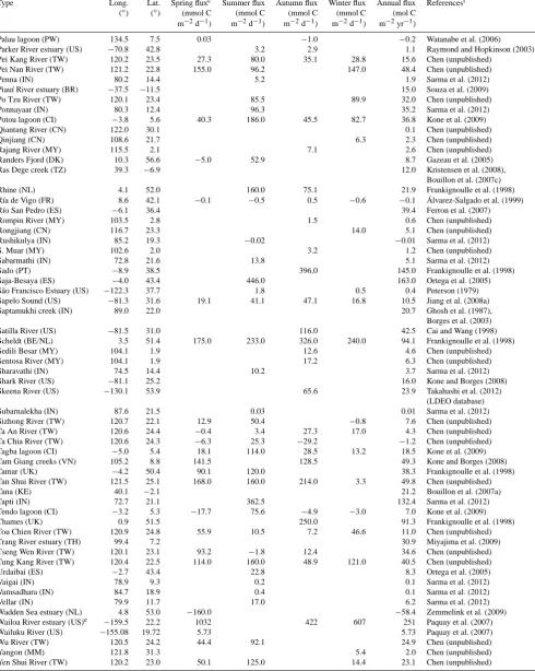
Table 1. Seasonal and annual sea-to-air fluxes of CO2in the world’s estuaries.

Type Long. Lat. Spring fluxc Summer flux Autumn flux Winter flux Annual flux Referencesf (◦) (◦) (mmol C (mmol C (mmol C (mmol C (mol C

m−2_d−1₎ _m−2_d−1₎ _m−2_d−1₎ _m−2_d−1₎ _m−2_yr−1₎

1-1 (fjord) (US)b −152.5 57.7 −1.8 1.8 0.001 Takahashi et al. (2012)

(LDEO database)

11-1 (fjord) (CA) −55.8 52.3 −2.1 −0.8 Takahashi et al. (2012)

(LDEO database) 14-1 (fjord) (IC) −23.2 66.2 −0.7 −7.0 −12.9 −4.8 −2.3 Takahashi et al. (2012)

(LDEO database)

14-2 (fjord) (IC) −23.6 66.1 −7.7 −2.8 Takahashi et al. (2012)

(LDEO database)

14-3 (fjord) (IC) −23.7 65.7 5.4 2.0 Takahashi et al. (2012)

(LDEO database)

14-4 (fjord) (IC) −24.1 65.6 −0.3 −0.1 Takahashi et al. (2012)

(LDEO database) 14-5 (fjord) (IC) −18.6 66.0 −48.2 −7.8 −11.2 −9.0 −7.0 Takahashi et al. (2012)

(LDEO database)

Aby lagoon (CI) −3.3 5.4 −10.1 1.2 −11.3 −4.1 −2.7 Kone et al. (2009)

Altamaha Sound (US) −81.3 31.3 57.8 127.0 79.7 28.5 26.8 Jiang et al. (2008a)

Ambalayaar (IN) 79.3 10.0 −0.02 −0.007 Sarma et al. (2012)

Amur River (RU) 141.1 52.9 0.1 1.5 0.3 Johnson et al. (2009)

(WOD09 database)

Ason (ES) −3.5 43.3 −3.0 −1.1 Ortega et al. (2005)

Aveiro lagoon (PT) −8.7 40.7 12.4 Borges and Frankignoulle

(unpublished)

Baitarani (IN) 86.9 20.5 20.7 7.6 Sarma et al. (2012)

Bancal (PH) 115.0 5.0 2.2 0.8 Chen (unpublished)

Bebar River (MY) 103.4 3.1 17.7 6.5 Chen (unpublished)

Bellamy (US) −70.9 43.1 −11.0 43.0 6.0 4.6 Hunt et al. (2011)

Betsiboka (MG) 46.3 −15.7 3.3 Ralison et al. (2008)

Bharatakulza (IN) 76.0 11.2 11.7 4.3 Sarma et al. (2012)

Bothnian Bay (FI) 21.0 63.0 3.5 Algesten et al. (2004)

Brazos River (US) −95.4 28.9 0.033 Zeng et al. (2011)

Brunei River (BN) 96.4 16.5 53.7 19.6 Chen (unpublished)

Cauvery (IN) 79.89 11.26 2.23 0.8 Sarma et al. (2012)

Chalakudi (IN) 76.18 10.69 12.86 4.70 Sarma et al. (2012)

Changjiang (Yangtze) (CN) 120.5 31.5 23.5 65.5 33.7 37.8 14.6 Zhai et al. (2007)

Chishui River (TW) 120.11 23.29 176 68.5 44.6 Chen (unpublished)

Chilka (lagoon) (IN) 85.5 19.1 9.8 141.0 27.5 Gupta et al. (2008)

Cho Shui River (TW) 120.3 23.9 651.0 13.4 121.0 Chen (unpublished)

Chung Kang River (TW) 120.8 24.7 45.8 53.4 28.8 144.0 24.8 Chen (unpublished)

Churchill River (CA) −94.2 58.8 1.2 −3.6 −0.4 Stainton (2009)

Citanduy River (ID) 108.8 −7.7 25.7d 9.4 Chen (unpublished)

Ciujung-Kragilan (ID) 106.4 −6.0 36.9d 13.5 Chen (unpublished)

Cocheco (US) −70.8 43.1 2.0 26.0 2.0 3.7 Hunt et al. (2011)

Cochin (IN) 76.0 9.5 267.0 65.0 60.6 Gupta et al. (2008)

Cross Sound (fjord) (US) −134.1 56.6 −0.2 45.1 8.2 Takahashi et al. (2012)

(LDEO database)

Doboy Sound (US) −81.3 31.4 15.2 47.4 51.0 16.0 11.9 Jiang et al. (2008a)

Douro (PT) −8.7 41.1 240.0 87.6 Frankignoulle et al. (1998)

Duplin River (US) −81.3 31.5 53.4 83.0 73.2 23.4 21.3 Wang and Cai (2004)

Ebrié lagoon (CI) −4.3 5.5 56.4 109.0 61.9 47.9 26.6 Kone et al. (2009)

Elbe (DE) 8.8 53.9 180.0 65.7 Frankignoulle et al. (1998)

Ems (DE) 6.9 53.4 110.0 40.2 Frankignoulle et al. (1998)

Endau River (MY) 103.6 2.7 1.0 0.4 Chen (unpublished)

Erh Jen River (TW) 120.2 22.9 68.5 11.1 26.5 12.9 Chen (unpublished)

Florida Bay (US) −80.8 25.0 1.7 Millero et al. (2001)

Fong Kang River (TW) 120.7 22.2 6.7 −17.9 18.0 0.8 Chen (unpublished)

Gaderu creek (IN) 82.3 16.8 56.0 20.4 Borges et al. (2003)

Gironde (FR) −1.1 45.6 110.0 110.0 65.0 50.0 30.6 Frankignoulle et al. (1998)

Godavari (IN) 82.3 16.7 8.0 Bouillon et al. (2003),

Sarma et al. (2012)

Godthåbsfjord (GL)e −51.9 64.1 −7.25 Rysgaard et al. (2012)

Golfo Almirante Montt −72.0 −52.1 −17.7d −6.5 Takahashi et al. (2012)

(5)

[image:5.595.59.544.83.714.2]

Table 1. Continued.

Type Long. Lat. Spring fluxc Summer flux Autumn flux Winter flux Annual flux Referencesf (◦₎ ₍◦₎ _{(mmol C} _{(mmol C} _{(mmol C} _{(mmol C} _{(mol C}

m−2d−1) m−2d−1) m−2d−1) m−2d−1) m−2yr−1)

Great Bay (US) −70.9 43.1 3.6 Hunt et al. (2011)

Guadalquivir (ES) −6.0 37.4 104.0 37.9 de la Paz et al. (2007)

Haldia (IN) 88.2 21.9 12.3 4.5 Sarma et al. (2012)

Hanjiang (CN) 116.8 23.4 0.9 0.3 Chen (unpublished)

Ho Ping River (TW) 121.8 24.3 5.3 22.0 68.5 11.7 Chen (unpublished)

Hooghly (IN) 88.0 22.0 31.8 −1.1 16.7 2.5 4.9 Mukhopadhyay et al. (2002)

Hou Lung River (TW) 120.8 24.6 72.9 9.3 7.6 21.0 10.1 Chen (unpublished)

Hsiu Ku Luan River (TW) 121.5 23.5 26.5 41.9 19.2 10.7 Chen (unpublished)

Hua Lien River (TW) 121.6 23.9 93.4 75.3 4.8 21.1 Chen (unpublished)

Hudson River estuary (US) −74.0 40.7 5.9 Raymond et al. (1997)

Isla Gordon (fjord) (CL) −68.9 −55.2 −1.2d −0.4 Takahashi et al. (2012)

(LDEO database)

Itacuruca creek, Sepetiba −44.0 −23.0 41.4 Ovalle et al. (1990),

(bay) (BR) Borges et al. (2003)

Jiulong Jiang 118.1 24.5 0.5 Dai et al. (2009)

(Xiamen Bay) (CN)

Jiulongjiang (CN) 118.0 24.5 4.3 1.6 Chen (unpublished)

Johor River (MY) 104.0 1.5 2.3 0.8 Chen (unpublished)

Kakinada Bay (IN) 82.3 16.7 3.0 Bouillon et al. (2003)

Kali (IN) 74.2 14.8 3.2 1.2 Sarma et al. (2012)

Kaneohe Bay and −157.8 21.5 1.5 Fagan and Mackenzie (2007)

stream (US)

Kao Ping River (TW) 120.4 22.5 98.1 51.8 30.5 12.4 17.6 Chen (unpublished)

Kapuas River (ID) 109.1 0.1 148.3 54.1 Chen (unpublished)

Kennebec River (US) −69.8 43.8 22.5 22.0 −0.2 −49.6 −0.5 Takahashi et al. (2012) (LDEO database)

Khura River estuary (TH) 98.3 9.2 35.7 Miyajima et al. (2009)

Kidogoweni creek 39.5 −4.4 154.4d 21.8 Bouillon et al. (2007b)

(Gazi Bay) (KE)

Kien Vang creeks(VN) 105.1 8.7 32.2 154.7 34.2 Kone and Borges (2008)

Klang River (MY) 101.4 3.0 7.7 2.8 Chen (unpublished)

Kobbe fjord (GL) −51.5 64.2 −2.7 −136.6 −2.6 −17.3 Ruiz−Halpern et al. (2010)

Kochi backwaters (IN) 76.4 10.0 8.1 2.9 Sarma et al. (2012)

Kola Bay (RU) 33.4 69.1 −2.5 −0.2 −3.5 −3.9 −0.9 Johnson et al. (2009)

(WOD09 database)

Krishna (IN) 81.1 15.8 6.8 2.5 Sarma et al. (2012)

Lan Yang River (TW) 121.8 24.7 65.5 66.0 23.2 18.8 Chen (unpublished)

Liminganlahti Bay (FI) 25.4 64.9 −0.9 −0.9 Silvennoinen et al. (2008)

Lin Pien River (TW) 120.5 22.4 44.4 54.5 49.0 18.0 Chen (unpublished)

Little Bay (US) −70.9 43.1 −5.1 33.9 3.9 4.0 Hunt et al. (2011)

Loire (FR) −2.2 47.2 155.0 64.4 Abril et al. (2003)

Luohe (CN) 115.6 22.9 0.1 0.022 Chen (unpublished)

Mahanadi (IN) 86.6 20.0 3.1 1.1 Sarma et al. (2012)

Mahisagar (IN) 72.6 22.1 10.2 3.7 Sarma et al. (2012)

Mandovi (IN) 73.8 15.7 18.1 6.6 Sarma et al. (2012)

Mandovi-Zuari (IN) 73.5 15.3 14.2 Sarma et al. (2001)

Matolo creek (KE) 40.1 −2.1 21.2 Bouillon et al. (2007a)

Mekong (VN) 106.5 10.0 30.8 Borges (unpublished)

Mempawah River (ID) 89.0 22.0 23.2 8.5 Chen (unpublished)

Mtoni (TZ) 39.3 −6.9 2.4 Kristensen et al. (2008)

Nagada creek (Papua 145.8 −5.2 43.6d 15.9 Borges et al. (2003)

New Guinea) (ID)

Nagavali (IN) 84.0 18.2 0.2 0.1 Sarma et al. (2012)

Nalonghe (CN) 112.0 21.8 10.1 3.7 Chen (unpublished)

Narmada (IN) 73.0 20.2 8.8 3.2 Sarma et al. (2012)

Netravathi (IN) 75.0 12.7 70.7 25.8 Sarma et al. (2012)

Norman’s Pond (BS) −76.1 23.8 13.8 5.0 Borges et al. (2003)

Orinoco River (VE) −62.3 8.6 31.8 11.6 Takahashi et al. (2012)

(LDEO database)

Oyster (US) −70.9 43.1 −17.2 51.5 2.5 4.5 Hunt et al. (2011)

Pa Chang River (TW) 120.1 23.3 29.9 94.2 34.8 19.3 Chen (unpublished)

(6)

[image:6.595.56.547.93.708.2]

Type Long. Lat. Spring fluxc Summer flux Autumn flux Winter flux Annual flux Referencesf (◦) (◦) (mmol C (mmol C (mmol C (mmol C (mol C

m−2d−1) m−2d−1) m−2d−1) m−2d−1) m−2yr−1)

Palau lagoon (PW) 134.5 7.5 0.03 −1.0 −0.2 Watanabe et al. (2006)

Parker River estuary (US) −70.8 42.8 3.2 2.9 1.1 Raymond and Hopkinson (2003)

Pei Kang River (TW) 120.2 23.5 27.3 80.0 35.1 28.8 15.6 Chen (unpublished)

Pei Nan River (TW) 121.2 22.8 155.0 96.2 147.0 48.4 Chen (unpublished)

Penna (IN) 80.2 14.4 5.2 1.9 Sarma et al. (2012)

Piauí River estuary (BR) −37.5 −11.5 15.0 Souza et al. (2009)

Po Tzu River (TW) 120.1 23.4 85.5 89.9 32.0 Chen (unpublished)

Ponnayaar (IN) 80.3 12.4 96.3 35.2 Sarma et al. (2012)

Potou lagoon (CI) −3.8 5.6 40.3 186.0 45.5 82.7 36.8 Kone et al. (2009)

Qiantang River (CN) 122.0 30.1 0.1 Chen (unpublished)

Qinjiang (CN) 108.6 21.7 6.3 2.3 Chen (unpublished)

Rajang River (MY) 115.5 2.1 7.1 2.6 Chen (unpublished)

Randers Fjord (DK) 10.3 56.6 −5.0 52.9 8.7 Gazeau et al. (2005)

Ras Dege creek (TZ) 39.3 −6.9 12.0 Kristensen et al. (2008),

Bouillon et al. (2007c)

Rhine (NL) 4.1 52.0 160.0 75.1 21.9 Frankignoulle et al. (1998)

Ría de Vigo (FR) 8.6 42.1 −0.1 −0.5 0.5 −0.6 −0.1 Álvarez-Salgado et al. (1999)

Río San Pedro (ES) −6.1 36.4 39.4 Ferron et al. (2007)

Rompin River (MY) 103.5 2.8 1.5 0.6 Chen (unpublished)

Rongjiang (CN) 116.7 23.3 14.0 5.1 Chen (unpublished)

Rushikulya (IN) 85.2 19.3 −0.02 −0.01 Sarma et al. (2012)

S. Muar (MY) 102.6 2.0 3.2 1.2 Chen (unpublished)

Sabarmathi (IN) 72.8 21.6 13.8 5.1 Sarma et al. (2012)

Sado (PT) −8.9 38.5 396.0 145.0 Frankignoulle et al. (1998)

Saja-Besaya (ES) −4.0 43.4 446.0 163.0 Ortega et al. (2005)

São Francisco Estuary (US) −122.3 37.7 1.8 0.5 0.4 Peterson (1979)

Sapelo Sound (US) −81.3 31.6 19.1 41.1 47.1 16.8 10.5 Jiang et al. (2008a)

Saptamukhi creek (IN) 89.0 22.0 20.7 Ghosh et al. (1987),

Borges et al. (2003)

Satilla River (US) −81.5 31.0 116.0 42.5 Cai and Wang (1998)

Scheldt (BE/NL) 3.5 51.4 175.0 233.0 326.0 240.0 94.1 Frankignoulle et al. (1998)

Sedili Besar (MY) 104.1 1.9 12.6 4.6 Chen (unpublished)

Sentosa River (MY) 104.1 1.9 17.2 6.3 Chen (unpublished)

Sharavathi (IN) 74.5 14.4 10.2 3.7 Sarma et al. (2012)

Shark River (US) −81.1 25.2 16.0 Kone and Borges (2008)

Skeena River (US) −130.1 53.9 65.6 23.9 Takahashi et al. (2012)

(LDEO database)

Subarnalekha (IN) 87.6 21.5 0.03 0.01 Sarma et al. (2012)

Sizhong River (TW) 120.7 22.1 12.9 50.4 −0.8 7.6 Chen (unpublished)

Ta An River (TW) 120.6 24.4 −0.4 3.4 27.3 17.0 4.3 Chen (unpublished)

Ta Chia River (TW) 120.6 24.3 −6.3 25.3 −29.2 −1.2 Chen (unpublished)

Tagba lagoon (CI) −5.0 5.4 18.1 114.0 28.5 13.2 18.5 Kone et al. (2009)

Tam Giang creeks (VN) 105.2 8.8 141.5 128.5 49.3 Kone and Borges (2008)

Tamar (UK) −4.2 50.4 90.1 120.0 38.3 Frankignoulle et al. (1998)

Tan Shui River (TW) 121.5 25.1 168.0 160.0 214.0 3.3 49.8 Chen (unpublished)

Tana (KE) 40.1 −2.1 21.2 Bouillon et al. (2007a)

Tapti (IN) 72.7 21.1 362.5 132.4 Sarma et al. (2012)

Tendo lagoon (CI) −3.2 5.3 −17.7 75.6 −4.9 −3.0 7.0 Kone et al. (2009)

Thames (UK) 0.9 51.5 250.0 91.3 Frankignoulle et al. (1998)

Tou Chien River (TW) 120.9 24.8 55.9 10.5 7.2 46.6 11.0 Chen (unpublished)

Trang River estuary (TH) 99.4 7.2 30.9 Miyajima et al. (2009)

Tseng Wen River (TW) 120.1 23.1 93.2 −1.8 12.4 34.6 Chen (unpublished)

Tung Kang River (TW) 120.4 22.5 114.0 160.0 48.9 121.0 40.5 Chen (unpublished)

Urdaibai (ES) −2.7 43.4 22.8 8.3 Ortega et al. (2005)

Vaigai (IN) 78.9 9.3 0.2 0.1 Sarma et al. (2012)

Vamsadhara (IN) 84.7 18.9 0.4 0.1 Sarma et al. (2012)

Vellar (IN) 79.9 11.7 17.0 6.2 Sarma et al. (2012)

Wadden Sea estuary (NL) 4.8 53.0 −160.0 −58.4 Zemmelink et al. (2009)

Wailoa River estuary (US)e −159.5 22.2 1032 422 607 251 Paquay et al. (2007)

Wailuku River (US) −155.08 19.72 5.73 5.73 Paquay et al. (2007)

Wu River (TW) 120.5 24.2 44.4 92.1 24.9 Chen (unpublished)

Yangon (MM) 121.8 31.3 5.4 2.0 Chen (unpublished)

(7)

Type Long. Lat. Spring fluxc Summer flux Autumn flux Winter flux Annual flux Referencesf

(◦) (◦) (mmol C (mmol C (mmol C (mmol C (mol C

m−2d−1) m−2d−1) m−2d−1) m−2d−1) m−2yr−1)

Yenisey (RU) 82.7 71.8 29.7 16.7 3.5 27.5 7.1 Johnson et al. (2009)

(WOD09 database)

York River (US) −76.4 37.2 10.0 29.0 16.7 6.5 5.6 Raymond et al. (2000)

Zhujiang (Pearl River) (CN) 113.5 22.5 60.2 70.7 47.0 22.2 6.9 Guo et al. (2009)

Zuari (IN) 74.0 15.3 6.4 2.3 Sarma et al. (2012)

a_{Positive fluxes indicate an emission of CO}

2from water to the atmosphere.

b_{BE: Belgium; BN: Brunei; BR: Brazil; BS: Bahamas; CI: Côte d’Ivoire; CL: Chile; CN: China; DE: Germany; DK: Denmark; ES: Spain; FI: Finland; FR: France; GL:}

Greenland; IC: Iceland; ID: Indonesia; IN: India; KE: Kenya; MG: Madagascar; MM: Myanmar; MY: Malaysia; NL: Netherlands; PH: Philippines; PT: Portugal; PW: Palau; RU: Russia; TH: Thailand; TW: Taiwan; TZ: Tunisia; UK: United Kingdom; US: United States; VE: Venezuela; VN: Vietnam.

c_{Spring: March–May; summer: June–August; autumn: September–November; winter: December–February.}

d_{Austral seasons.} e_{Not used in the calculation.}

f_{LDEO: Lamont-Doherty Earth Observatory; WOD09: World Ocean Database 2009.}

[image:7.595.70.525.262.484.2]

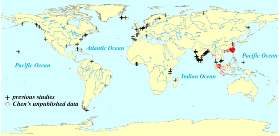
1 Fig. 1. Distribution of estuaries studied.

2

3

Fig. 1. Distribution of estuaries studied.

estuaries. Factors affecting gas exchange coefficients include wind speed, tidal current and bottom stress, whereas the wind speed is the most considered. It is important to point out that this paper deals mostly with published results. It is not possi-ble to re-do the flux calculations, say, based on the same gas exchange coefficient, as the original data were not provided in the papers cited. Further, there is a lack of temporal cover-age as previous studies (Bozec et al., 2011; Dai et al., 2009; Kitidis et al., 2012) have demonstrated short-term changes in pCO2at scales of days or less. Yet, typically data on such a scale are limited to only a few cruises. The lack of seasonal-ity in the numerically averaged fluxes is almost certainly an artifact influenced by averaging all available data.

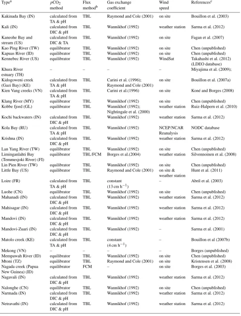
Figure 2 presents the pCO2 and CO2 fluxes per unit area in the upper, mid- and lower estuaries worldwide.

Up-per, mid-, and lower estuaries are defined as those areas of estuaries with salinities below 2, between 2 and 25, and above 25, respectively, as salinity data are the most read-ily available. Otherwise, divisions are made based approx-imately on one-third of the distance from the point where the river starts to widen to the river mouth. Almost all estu-aries outside of the Arctic region except for only a few re-lease CO2to the atmosphere. Unsurprisingly, upper estuar-ies, where the riverine effect is the strongest (Kempe, 1979, 1982; Chen et al., 2012), have the highest pCO2 (numer-ical average = 5026±6190 µatm) and the highest sea-to-air CO2 flux (numerical average = 39.0±55.7 mol C m−2yr−1, where the positive sign indicates that the seawater is losing CO2); these are followed by the mid-estuaries (numerically averaged pCO2= 2230±2725 µatm; numerically averaged

(8)

[image:8.595.55.547.89.710.2]

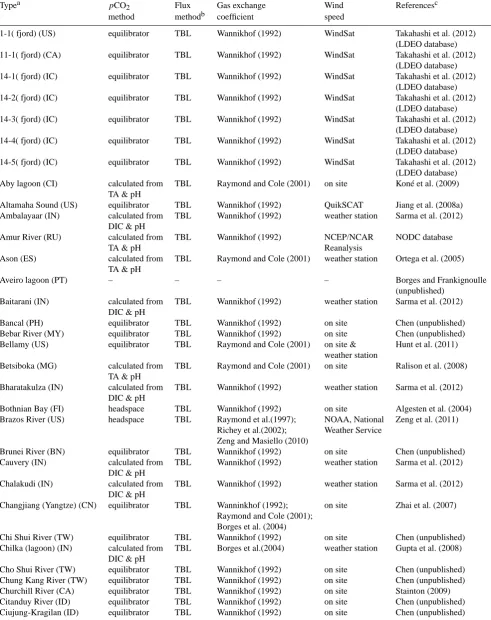
Table 2. ThepCO2and flux method, the gas exchange coefficient and the wind speed in the world’s estuaries.

Typea pCO2 Flux Gas exchange Wind Referencesc

method methodb coefficient speed

1-1( fjord) (US) equilibrator TBL Wannikhof (1992) WindSat Takahashi et al. (2012)

(LDEO database)

11-1( fjord) (CA) equilibrator TBL Wannikhof (1992) WindSat Takahashi et al. (2012)

(LDEO database)

14-1( fjord) (IC) equilibrator TBL Wannikhof (1992) WindSat Takahashi et al. (2012)

(LDEO database)

Aby lagoon (CI) calculated from TBL Raymond and Cole (2001) on site Koné et al. (2009)

TA & pH

Altamaha Sound (US) equilibrator TBL Wannikhof (1992) QuikSCAT Jiang et al. (2008a)

Ambalayaar (IN) calculated from TBL Wannikhof (1992) weather station Sarma et al. (2012)

DIC & pH

Amur River (RU) calculated from TBL Wannikhof (1992) NCEP/NCAR NODC database

TA & pH Reanalysis

Ason (ES) calculated from TBL Raymond and Cole (2001) weather station Ortega et al. (2005)

TA & pH

Aveiro lagoon (PT) – – – – Borges and Frankignoulle

(unpublished)

Baitarani (IN) calculated from TBL Wannikhof (1992) weather station Sarma et al. (2012)

DIC & pH

Bancal (PH) equilibrator TBL Wannikhof (1992) on site Chen (unpublished)

Bebar River (MY) equilibrator TBL Wannikhof (1992) on site Chen (unpublished)

Bellamy (US) equilibrator TBL Raymond and Cole (2001) on site & Hunt et al. (2011)

weather station

Betsiboka (MG) calculated from TBL Raymond and Cole (2001) on site Ralison et al. (2008)

TA & pH

Bharatakulza (IN) calculated from TBL Wannikhof (1992) weather station Sarma et al. (2012)

DIC & pH

Bothnian Bay (FI) headspace TBL Wannikhof (1992) on site Algesten et al. (2004)

Brazos River (US) headspace TBL Raymond et al.(1997); NOAA, National Zeng et al. (2011)

Richey et al.(2002); Weather Service Zeng and Masiello (2010)

Brunei River (BN) equilibrator TBL Wannikhof (1992) on site Chen (unpublished)

Cauvery (IN) calculated from TBL Wannikhof (1992) weather station Sarma et al. (2012)

DIC & pH

Chalakudi (IN) calculated from TBL Wannikhof (1992) weather station Sarma et al. (2012)

DIC & pH

Changjiang (Yangtze) (CN) equilibrator TBL Wanninkhof (1992); on site Zhai et al. (2007)

Raymond and Cole (2001); Borges et al. (2004)

Chi Shui River (TW) equilibrator TBL Wannikhof (1992) on site Chen (unpublished)

Chilka (lagoon) (IN) calculated from TBL Borges et al.(2004) weather station Gupta et al. (2008) DIC & pH

Cho Shui River (TW) equilibrator TBL Wannikhof (1992) on site Chen (unpublished)

Chung Kang River (TW) equilibrator TBL Wannikhof (1992) on site Chen (unpublished)

Churchill River (CA) equilibrator TBL Wannikhof (1992) on site Stainton (2009)

Citanduy River (ID) equilibrator TBL Wannikhof (1992) on site Chen (unpublished)

(9)

[image:9.595.59.542.87.712.2]

Typea pCO₂ Flux Gas exchange Wind Referencesc

Cocheco (US) equilibrator TBL Raymond and Cole (2001) on site & Hunt et al. (2011)

weather station

Cochin (IN) calculated from TBL Borges et al. (2004) on site Gupta et al. (2009)

DIC & pH

Cross Sound equilibrator TBL Wannikhof (1992) WindSat Takahashi et al. (2012)

(fjord) (US) (LDEO database)

Doboy Sound (US) equilibrator TBL Wannikhof (1992) QuikSCAT Jiang et al. (2008a)

Douro (PT) calculated from TBL/FCM constant on site Frankignoulle et al. (1998)

TA & pH/ (8 cm h−1)/–

equilibrator

Duplin River(US) equilibrator TBL Raymond et al. (2000) on site Wang and Cai (2004)

Ebrié lagoon (CI) calculated from TBL Raymond and Cole (2001) on site Koné et al. (2009)

TA & pH

Elbe (DE) calculated from TBL/FCM constant on site Frankignoulle et al. (1998)

TA & pH/ (8 cm h−1)/–

equilibrator

Ems (DE) calculated from TBL/FCM constant on site Frankignoulle et al. (1998)

TA & pH/ (8 cm h−1)/–

equilibrator

Endau River (MY) equilibrator TBL Wannikhof (1992) on site Chen (unpublished)

Erh Jen River (TW) equilibrator TBL Wannikhof (1992) on site Chen (unpublished)

Florida Bay (US) equilibrator TBL constant – Millero et al. (2001)

(4 cm h−1)

Fong Kang River (TW) equilibrator TBL Wannikhof (1992) on site Chen (unpublished)

Gaderu creek(IN) equilibrator FCM – on site Borges et al. (2003)

Gironde (FR) calculated from TBL/FCM constant on site Frankignoulle et al. (1998)

TA & pH/ (8 cm h−1)/–

equilibrator

Godavari (IN) equilibrator/ TBL Raymond and Cole (2001); on site; Bouillon et al. (2003);

calculated from Wannikhof (1992) weather station Sarma et al. (2012)

DIC & pH

Golfo Almirante equilibrator TBL Wannikhof (1992) WindSat Takahashi et al. (2012)

Montt (fjord) (CL) (LDEO database)

Great Bay (US) equilibrator TBL Raymond and Cole (2001) on site & Hunt et al. (2011)

weather station

Guadalquivir (ES) equilibrator TBL O’Connor and Dobbins on site de La Paz et al. (2007)

(1958); Borges et al. (2004); Cariniet al. (1996); Clark et al. (1995); Wannikhof (1992)

Haldia (IN) calculated from TBL Wannikhof (1992) weather station Sarma et al. (2012)

DIC & pH

Hanjiang (CN) equilibrator TBL Wannikhof (1992) on site Chen (unpublished)

Ho Ping River (TW) equilibrator TBL Wannikhof (1992) on site Chen (unpublished)

Hooghly (IN) headspace TBL Wannikhof (1992) on site Mukhopadhyay et al. (2002)

Hou Lung River (TW) equilibrator TBL Wannikhof (1992) on site Chen (unpublished)

Hsiu Ku Luan River (TW) equilibrator TBL Wannikhof (1992) on site Chen (unpublished)

Hua Lien River (TW) equilibrator TBL Wannikhof (1992) on site Chen (unpublished)

Hudson River estuary (US) headspace TBL Clark et al.(1994) weather station Raymond et al. (1997)

Isla Gordon (fjord) (CL) equilibrator TBL Wannikhof (1992) WindSat Takahashi et al. (2012)

(LDEO database)

Itacuraca creek equilibrator FCM – on site Ovalle et al. (1990),

Sepetiba Bay (BR) Borges et al. (2003)

Jiulong Jiang equilibrator TBL Wannikhof (1992) on site Dai et al. (2009)

(Xiamen Bay) (CN)

Jiulongjiang (CN) equilibrator TBL Wannikhof (1992) on site Chen (unpublished)

(10)

[image:10.595.57.545.84.723.2]

Kakinada Bay (IN) calculated from TBL Raymond and Cole (2001) on site Bouillon et al. (2003) TA & pH

Kali (IN) calculated from TBL Wannikhof (1992) weather station Sarma et al. (2012)

DIC & pH

Kaneohe Bay and calculated from TBL Wannikhof (1992) on site Fagan et al. (2007)

stream (US) DIC & TA

Kao Ping River (TW) equilibrator TBL Wannikhof (1992) on site Chen (unpublished)

Kapuas River (ID) equilibrator TBL Wannikhof (1992) on site Chen (unpublished)

Kennebec River (US) equilibrator TBL Wannikhof (1992) WindSat Takahashi et al. (2012)

(LDEO database)

Khura River – – – – Miyajima et al. (2009);

estuary (TH)

Kidogoweni creek calculated from TBL Carini et al. (1996); on site Bouillon et al. (2007a)

(Gazi Bay) (KE) TA & pH Raymond and Cole (2001)

Kien Vang creeks (VN) calculated from TBL Carini et al.(1996) on site Koné and Borges (2008)

TA & pH

Klang River (MY) equilibrator TBL Wannikhof (1992) on site Chen (unpublished)

Kobbe fjord (GL) equilibrator TBL Wannikhof (1992); weather station Ruiz-Halpern et al. (2010) Nightingale et al. (2000)

Kochi backwaters (IN) calculated from TBL Wannikhof (1992) weather station Sarma et al. (2012) DIC & pH

Kola Bay (RU) calculated from TBL Wannikhof (1992) NCEP/NCAR NODC database

TA & pH Reanalysis

Krishna (IN) calculated from TBL Wannikhof (1992) weather station Sarma et al. (2012)

DIC & pH

Lan Yang River (TW) equilibrator TBL Wannikhof (1992) on site Chen (unpublished)

Liminganlahti Bay equilibrator TBL/FCM Borges et al.(2004) weather station Silvennoinen et al. (2008) (Temmesjoki River) (FI)

Lin Pien River (TW) equilibrator TBL Wannikhof (1992) on site Chen (unpublished)

Little Bay (US) equilibrator TBL Raymond and Cole (2001) on site & Hunt et al. (2011) weather station

Loire (FR) calculated from TBL constant – Abril et al. (2003)

TA & pH (13 cm h−1)

Luohe (CN) equilibrator TBL Wannikhof (1992) on site Chen (unpublished)

Mahanadi (IN) calculated from TBL Wannikhof (1992) weather station Sarma et al. (2012)

DIC & pH

Mahisagar (IN) calculated from TBL Wannikhof (1992) weather station Sarma et al. (2012)

DIC & pH

Mandovi (IN) calculated from TBL Wannikhof (1992) weather station Sarma et al. (2012)

DIC & pH

Mandovi-Zuari (IN) calculated from TBL Wannikhof (1992) – Sarma et al. (2001)

DIC & pH

Matolo creek (KE) calculated from TBL constant – Bouillon et al (2007b)

TA & pH (4 cm h−1)

Mekong (VN) – – – – Borges (unpublished)

Mempawah River (ID) equilibrator TBL Wannikhof (1992) on site Chen (unpublished)

Mtoni (TZ) equilibrator TBL Raymond and Cole (2001) on site Kristensen et al. (2008)

Nagada creek (Papua equilibrator FCM – on site Borges et al. (2003)

New Guinea) (ID)

Nagavali (IN) calculated from TBL Wannikhof (1992) weather station Sarma et al. (2012)

DIC & pH

Nalonghe (CN) equilibrator TBL Wannikhof (1992) on site Chen (unpublished)

Narmada (IN) calculated from TBL Wannikhof (1992) weather station Sarma et al. (2012)

DIC & pH

Netravathi (IN) calculated from TBL Wannikhof (1992) weather station Sarma et al. (2012)

(11)

[image:11.595.59.543.86.714.2]

Norman’s Pond (BS) equilibrator FCM – on site Borges et al. (2003)

Orinoco River (VE) equilibrator TBL Wannikhof (1992) WindSat Takahashi et al. (2012)

(LDEO database)

Oyster (US) equilibrator TBL Raymond and Cole (2001) on site & Hunt et al. (2011)

weather station

Pa Chang River (TW) equilibrator TBL Wannikhof (1992) on site Chen (unpublished)

Pahang River (MY) equilibrator TBL Wannikhof (1992) on site Chen (unpublished)

Palau lagoon (PW) calculated from TBL McGillis et al. (2001) NOAA station Watanabe et al. (2006)

DIC & TA

Parker River estuary (US) equilibrator TBL constant – Raymond and Hopkinson

(4 cm h−1)

Pei Kang River (TW) (2003) equilibrator TBL Wannikhof (1992) on site Chen (unpublished)

Pei Nan River (TW) equilibrator TBL Wannikhof (1992) on site Chen (unpublished)

Penna (IN) calculated from TBL Wannikhof (1992) weather station Sarma et al. (2012)

DIC & pH

Piauí River calculated from TBL range (1–3 cm h−1) on site Souza et al. (2009)

estuary (BR) DIC & pH

Po Tzu River (TW) equilibrator TBL Wannikhof (1992) on site Chen (unpublished)

Ponnayaar (IN) equilibrator TBL Wannikhof (1992) on site Sarma et al. (2012)

Potou lagoon (CI) calculated from TBL Raymond and Cole (2001) on site Koné et al. (2009)

TA & pH

Qiantang River (CN) equilibrator TBL Wannikhof (1992) on site Chen (unpublished)

Qinjiang (CN) equilibrator TBL Wannikhof (1992) on site Chen (unpublished)

Rajang River (MY) equilibrator TBL Wannikhof (1992) on site Chen (unpublished)

Randers Fjord (DK) equilibrator TBL Borges et al. (2004) on site Gazeau et al. (2005)

Ras Dege creek (TZ) equilibrator/ TBL Raymond and Cole (2001) on site Kristensen et al. (2008);

calculated from Bouillon et al (2007c)

TA & pH

Rhine (NL) calculated from TBL/FCM constant on site Frankignoulle et al. (1998)

TA & pH/ (8 cm h−1)/–

equilibrator

Ría de Vigo (FR) calculated from TBL Liss and Mervilat (1986); estimated Álvarez-Salgado et al.

TA & pH Woolf and Thorpe (1991) (1999)

Río San Pedro (ES) headspace TBL Clark et al. (1995); weather station Ferrón et al. (2007)

Carini et al. (1996); Kremer et al. (2003); Borges et al. (2004)

Rompin River (MY) equilibrator TBL Wannikhof (1992) on site Chen (unpublished)

Rongjiang (CN) equilibrator TBL Wannikhof (1992) on site Chen (unpublished)

Rushikulya (IN) calculated from TBL Wannikhof (1992) weather station Sarma et al. (2012)

DIC & pH

S. Muar (MY) equilibrator TBL Wannikhof (1992) on site Chen (unpublished)

Sabarmathi (IN) calculated from TBL Wannikhof (1992) weather station Sarma et al. (2012)

DIC & pH

Sado (PT) calculated from TBL/FCM constant on site Frankignoulle et al. (1998)

TA & pH/ (8 cm h−1)/–

equilibrator

Saja-Besaya (ES) calculated from TBL Raymond and Cole (2001) weather station Ortega et al. (2005) TA & pH

São Francisco calculated from TBL range (4–8 cm h−1) – Peterson (1979)

Estuary (US) TA & pH

Sapelo Sound (US) equilibrator TBL Jiang et al. (2008a) QuikSCAT Jiang et al. (2008a)

Saptamukhi creek (IN) calculated from FCM – on site Ghosh et al. (1987);

TA & pH/ Borges et al. (2003)

equilibrator

(12)

[image:12.595.51.548.77.727.2]

Scheldt (BE/NL) calculated from TBL/FCM constant on site Frankignoulle et al. (1998)

TA & pH/ (8 cm h−1)/–

equilibrator

Sedili Besar (MY) equilibrator TBL Wannikhof (1992) on site Chen (unpublished)

Sentosa River (MY) equilibrator TBL Wannikhof (1992) on site Chen (unpublished)

Sharavathi (IN) calculated from TBL Wannikhof (1992) weather station Sarma et al. (2012)

DIC & pH

Shark River (US) calculated from TBL Carini et al. (1996) on site Koné and Borges (2008)

TA & pH

Skeena River (US) equilibrator TBL Wannikhof (1992) WindSat Takahashi et al. (2012)

(LDEO database)

Subarnalekha (IN) calculated from TBL Wannikhof (1992) weather station Sarma et al. (2012)

DIC & pH

Sizhong River (TW) equilibrator TBL Wannikhof (1992) on site Chen (unpublished)

Ta An River (TW) equilibrator TBL Wannikhof (1992) on site Chen (unpublished)

Ta Chia River (TW) equilibrator TBL Wannikhof (1992) on site Chen (unpublished)

Tagba lagoon (CI) calculated from TBL Raymond and Cole (2001) on site Koné et al. (2009)

TA & pH

Tam Giang creeks (VN) calculated from TBL Carini et al. (1996) on site Koné and Borges (2008)

TA & pH

Tamar (UK) calculated from TBL/FCM constant on site Frankignoulle et al. (1998)

TA & pH/ (8 cm h−1)/–

equilibrator

Tan Shui River (TW) equilibrator TBL Wannikhof (1992) on site Chen (unpublished)

Tana (KE) calculated from TBL constant (4 cm h−1) – Bouillon et al (2007b)

TA & pH

Tapti (IN) calculated from TBL Wannikhof (1992) weather station Sarma et al. (2012)

DIC & pH

Tendo lagoon (CI) calculated from TBL Raymond and Cole (2001) on site Koné et al. (2009)

TA & pH

Thames (UK) calculated from TBL/FCM constant on site Frankignoulle et al. (1998)

TA & pH/ (8 cm h−1)/–

equilibrator

Tou Chien River (TW) equilibrator TBL Wannikhof (1992) on site Chen (unpublished)

Trang River – – – – Miyajima et al. (2009);

estuary (TH)

Tseng Wen River (TW) equilibrator TBL Wannikhof (1992) on site Chen (unpublished)

Tung Kang River (TW) equilibrator TBL Wannikhof (1992) on site Chen (unpublished)

Urdaibai (ES) calculated from TBL Raymond and Cole (2001) weather station Ortega et al. (2005) TA & pH

Vaigai (IN) calculated from TBL Wannikhof (1992) weather station Sarma et al. (2012)

DIC & pH

Vamsadhara (IN) calculated from TBL Wannikhof (1992) weather station Sarma et al. (2012)

DIC & pH

Vellar (IN) calculated from TBL Wannikhof (1992) weather station Sarma et al. (2012)

DIC & pH

Wadden Sea estuary (NL) calculated from TBL Wannikhof (1992) – Zemmelink et al. (2009)

DIC & TA

Wu River (TW) equilibrator TBL Wannikhof (1992) on site Chen (unpublished)

Yangon (MM) equilibrator TBL Wannikhof (1992) on site Chen (unpublished)

Yen Shui River (TW) equilibrator TBL Wannikhof (1992) on site Chen (unpublished)

Yenisey (RU) calculated from TBL Wannikhof (1992) NCEP/NCAR NODC database

TA & pH Reanalysis

York River (US) equilibrator TBL Clark et al. (1994); – Raymond et al. (2000)

(13)

[image:13.595.89.503.82.159.2]

Zhujiang (Pearl equilibrator TBL Wannikhof (1992); – Guo et al. (2009)

River) (CN) Borges et al. (2004)

Zuari (IN) calculated from TBL Wannikhof (1992) weather station Sarma et al. (2012) DIC & pH

a_{BE: Belgium; BN: Brunei; BR: Brazil; BS: Bahamas; CI: Côte d’Ivoire, CL: Chile; CN: China; DE: Germany; DK: Denmark; ES: Spain; FI:}

Finland; FR: France; GL: Greenland; IC: Iceland; ID: Indonesia; IN: India; KE: Kenya; MG: Madagascar; MM: Myanmar; MY: Malaysia; NL: Netherlands; PH: Philippines; PT: Portugal; PW: Palau; RU: Russia; TH: Thailand; TW: Taiwan; TZ: Tunisia; UK: United Kingdom; US: United States; VE: Venezuela; VN: Vietnam.

b_{TBL: thin boundary layer method; FCM: floating chamber method.}

c_{LDEO: Lamont-Doherty Earth Observatory; WOD09: World Ocean Database 2009.}

66

x103atm 0 2 4 6 8 10 12 14 10

20 30 40

Upper estuaries

x103atm 0 3 6 9 10

20 30 40

x103_

atm 0.0 0.5 1.0 1.5 10

20 30 40

>14 >9 >1.5

Mid estuaries Lower estuaries

mol C m-2

yr-1

<0 0 60 120 180 10

20 30 40 50

mol C m-2

yr-1

-20 0 40 80 120 10

20 30 40 50

mol C m-2

yr-1

<0 0 10 20 30 40 50 >50 10 20 30 40 50 5026± 6190 n=62 39.0± 55.7 n=68 2230± 2725 n=68 17.5± 34.2 n=69 723± 957 n=57 8.4± 14.3 n=66 >180 >120

number number number

[image:13.595.52.287.237.394.2]

1

Fig.2. CO2 flux in (a) upper, (b) mid and (c) lower estuaries.

2

Fig. 2. CO2flux in (a) upper, (b) mid- and (c) lower estuaries.

flux = 17.5±34.2 mol C m−2_yr−1_{). Lower estuaries have the} lowestpCO2(numerical average = 723±957 µatm) and CO2 flux (numerical average = 8.4±14.3 mol C m−2yr−1). Ex-cept for those of the upper estuaries, these pCO2 values compare favorably with those found by Chen et al. (2012), which were 3033, 2277, and 692 µatm for the upper, mid- and lower estuaries, respectively. This study yields much higher pCO2 values for upper estuaries mainly because new data from Asia are associated with highpCO2values. The fluxes obtained by Chen et al. (2012), however, are higher. Their values are 68.5, 37.4 and 9.92 mol C m−2yr−1for the upper, mid- and lower estuaries, respectively. The seeming incon-sistency among results is discussed below.

Figure 3 displays histograms of reported daily CO2fluxes per unit area in different seasons and the annual flux per unit area in the world’s estuaries. Little seasonality is observed, except that the flux is lower in the winter when thepCO2 is usually lower, perhaps because the temperature is lower than other seasons. The flux is only marginally higher in summer than in spring or autumn. The numerical average an-nual flux per unit area is 16.5±27.7 mol C m−2yr−1, which is significantly lower than that, 23.9±33.1 mmol C m−2d−1, obtained by Chen et al. (2012). The numerical average

an-67

mmol C m-2

d-1

-80 0 80 160 200 10 20 30 40 Spring >200 < -80 46.3± 95.4 n=63

mmol C m-2

d-1

-40 0 40 120 200 280 10 20 30 40 Summer >280 52.0± 73.9 n=96

mmol C m-2

d-1

-40 0 40 120 200 280

Autumn

<-40 >280

47.2± 88.8 n=65

mmol C m-2

d-1

-25 0 50 100 150 10 20 30 40 Winter >150 35.0± 51.3 n=56

mol C m-2 yr-1

-20 0 20 40 60 80 100

Annual

< -20 >100

16.5± 27.7 n=165 40 30 20 10 40 20 60 80 number number number number number <-25 1

Figure 3. Histogram of reported daily CO2 fluxes per unit area in different seasons and the annual flux of

2

world's estuaries. 3

Fig. 3. Histogram of reported daily CO2fluxes per unit area in

dif-ferent seasons and the annual flux of the world’s estuaries.

nual flux per unit area, however, is not used to calculate the global release of CO2because small estuaries dominate the numerical average, but they contribute relatively little to the total flux. Important to note is that there is a lack of tempo-ral coverage in most of the data sets although previous stud-ies (Bozec et al., 2011; Dai et al., 2009; Kitidis et al., 2012) have demonstrated short-term changes inpCO2at scales of days or less. Yet, typically data on such a scale are limited to only a few cruises. The lack of seasonality in the numerically averaged fluxes is almost certainly an artifact influenced by averaging all available data.

[image:13.595.306.545.237.421.2]

(14)

68 mmol C m-2_d-1

-25 0 50 100 150 225 10

20 30 40

mmol C m-2 d-1 -25 0 50 100 150 200 250

10 20 30 40

0o-23.5oN

mmol C m-2_d-1

<0 0 30 60 90 120 150 10 20 30 40 38.8± 55.4 n=80

23.5o -50oN > 50oN

>250 >150 63.3± 100.7 n=47 35.9± 91.2 n=24 <-25 >225 number number

number _{> 50}o

S

mmol C m-2_d-1

0 4 8 12 16 18 5

9.5± 11.7 n=2

23.5oS-0o

mmol C m-2 d-1 0 20 40 60 80 100 120 5 44.1± 29.3 n=11 number number 1

Figure 4. Histogram of reported annual CO2 fluxes of world's estuaries in various latitude bands. 2

[image:14.595.51.283.61.252.2]

3

Fig. 4. Histogram of reported annual CO2fluxes of the world’s

es-tuaries in various latitude bands.

Chen et al. (2012) obtained 65.5±78.1 mmol C m−2d−1 – a slightly higher value than obtained in this study – between 23.5◦N and 23.5◦S. The values of Chen et al. (2012) are 67.4±108 mmol C m−2d−1 between 23.5 and 50◦N and 59.2±80 mmol C m−2d−1 north of 50◦N, however, significantly higher than those obtained herein. Notably, most other investigations have presented fluxes higher than those that were presented by Chen et al. (2012).

The fact that the annual average flux herein is lower than those reported previously, despite the fact the averagepCO2 is higher, warrants discussion. It follows mainly from the fact that many data from the low-latitude bands in Asia have been added, and these areas are mostly areas of low wind en-ergy. Figure 5 plots the wind energy potential, which is, like the air–sea gas exchange rate, a quadratic function of wind speed. The areas of high wind energy at low latitudes are con-centrated in the dry Middle East and northeastern, northern and northwestern Africa with few rivers, and therefore few estuaries. For example, the total area of the estuaries in the Red Sea region is almost zero (Table 3; Laruelle et al., 2013). Accordingly, the global average CO2flux herein is substan-tially affected by estuaries in areas of low wind energy, and therefore of low CO2flux.

The 50 newly considered estuaries in Taiwan, south-ern China and Southeast Asia, all at low latitudes, have lower fluxes than determined from previously obtained re-sults (Table 1), which include many data for European rivers. For instance, only 2 of the 19 estuaries that were con-sidered by Abril and Borges (2005), who published per-haps the first global study of CO2 emissions from estu-aries, are outside Europe and the eastern seaboard of the USA. Those authors found a global CO2flux per unit area of 35.7 mol C m−2yr−1, which is more than triple the value obtained in this study. This finding does not imply that

Eu-ropean rivers have higherpCO2: they do not. Rather, Eu-rope has more windy coasts than elsewhere in the world, and especially Asia. Parts of these higher fluxes may have resulted from higher wind speed. As mentioned above, the wind potential is a quadratic function of wind speed, as is the 1992 Wanninkhof air–sea CO2 exchange equation. It is important to point out, however, that the water turbulence is an importance factor for gas transfer velocity in low wind speed regions, but little data is available. We have com-pared the Wanninkhof (1992) quadratic equation (k660=

0.31×U102) with other equations such as those of Raymond and Cole (2001), Borges et al. (2004), Ho et al. (2011), and Jiang et al. (2008a). Using Wanninkhof’s (1992) quadratic equation may underestimate flux, although the value is simi-lar to that of Ho et al. (2011) at low wind speed (<5 m s−1). Note that there is no theoretical basis for the above equations as most are based on curve fitting techniques. Since we do not have data to show which equation is the best, we have chosen the Wanninkhof quadratic equation, which most ref-erences we cited used. Due to the fact that using different air–sea exchange equations results in large uncertainties, and that there is no universally accepted equation, the above con-clusion can only be deemed preliminary. The meanpCO2 of European estuaries is roughly 1600 µatm, whereas that of Asian estuaries is much higher, around 4000 µatm. Yet, the mean wind speed on European coasts is approximately 4 m s−1, compared with about 1.6 m s−1on Asian coasts. The resulting CO2 fluxes for European estuaries average about 16.9 mol C m−2yr−1 vs. a much lower 8.1 mol C m−2yr−1 for Asian estuaries (Table 3; Fig. 6) despite their higher pCO2.

In the above calculation, the areas of groups of es-tuaries are taken from the most recent and comprehen-sive work of Laruelle et al. (2013), which divided the world into 45 regions and calculated a total estuarine area of 1.012×106km2, slightly smaller than the value of 1.067×106km2given in Laruelle et al. (2010). Table 3 lists the total surface area in each of the 45 regions and the numer-ically averaged CO2flux per unit area for each region. Our global flux calculation is based on the sum of regional fluxes for these 45 zones (area multiplied by zonal average CO2flux (mol C m−2yr−1)). These 165 estuaries are compartmental-ized into 35 regions, and the numerically averaged CO2flux per unit area is calculated. For 10 regions without data, the mean flux for the same classification region is used (Table 3). The outgassing of CO2in global estuaries is 0.094 Pg C yr−1, and is about 31 % of the global riverine organic carbon flux (Seitzinger et al., 2010). This compares with the 48 % of or-ganic carbon released as CO2from estuaries and inland wa-ters (Tranvik et al., 2009).

(15)

[image:15.595.52.547.81.540.2]

Table 3. Areas and air–sea fluxes of CO₂in estuaries and continental shelves by biogeochemical provinces (Laruelle et al., 2013).

MARCATS Continent Ocean System Class Estuarine Average CO2 CO2 Shelf Average CO2 CO2 segment name surface flux (mol C flux surface flux (mol C flux number (103km2) m−2yr−1) (Tg C (103km2) m−2yr−1) (Tg C yr−1) yr−1)

1 NA PA Northeastern Pacific Subpolar 33.9 10.71 (n= 3) 4.36 461 −3.51 (n= 3) −19.40 2 NA/OC PA Californian Current EBC 8.9 0.93 (n= 3) 0.10 214 −2.22 (n= 3) −5.69 3 NA PA Tropical Eastern Pacific Tropical 6.2 14.47 1.08 198 −0.05 (n= 2) −0.13 4 SA PA Peruvian Upwelling Current EBC 4.2 34.71 1.75 143 −0.62 (n= 4) −1.07 5 SA AT South America Subpolar 22 −3.46 (n= 2) −0.91 1230 −3.25 (n= 3) −47.98 6 SA AT Brazilian Current WBC 26.3 28.20 (n= 2) 8.90 521 3.97 (n= 1) 24.81 7 SA AT Tropical Western Atlantic Tropical 13.4 11.60 (n= 1) 1.87 517 −12.78 (n= 1) −79.26 8 NA AT Caribbean Sea Tropical 26.2 5.04 (n= 1) 1.58 344 0.66 (n= 1) 2.74 9 NA AT Gulf of Mexico Marginal Sea 31.9 8.02 (n= 2) 3.07 544 −0.19 (n= 2) −1.26 10 NA AT Florida Upwelling WBC 34 9.81 (n= 15) 4.00 858 −1.10 (n= 4) −11.27 11 NA AT Sea of Labrador Subpolar 36.1 −0.76 (n= 1) −0.33 395 −2.11 (n= 1) −10.02 12 NA AT Hudson Bay Marginal Sea 39 −0.44 (n= 1) −0.20 1064 0.84 (n= 1) 10.73 13 NA AR Canadian Archipelago Polar 163.7 −1.08 −2.11 1177 −4.06 (n= 2) −57.34 14 NA AR Northern Greenland Polar 24.1 −2.05 (n= 5) −0.59 614 6.14 (n= 1) 45.20 15 NA AR Southern Greenland Polar 8.8 −1.08 −0.11 270 −5.95 (n= 1) −19.29 16 EU AR Norwegian Basin Polar 17 −17.30 (n= 1) −3.53 171 −3.63 (n= 1) −7.45 17 EU AT Northeastern Atlantic Marginal Sea 37.6 37.73 (n= 8) 17.02 1112 −1.04 (n= 2) −13.88 18 EU AT Baltic Sea Marginal Sea 26.3 1.28 (n= 2) 0.40 383 −1.95 (n= 1) −8.96 19 EU AT Iberian Upwelling EBC 12.7 58.75 (n= 10) 8.95 283 −1.33 (n= 5) −4.51 20 EU AT Mediterranean Sea Marginal Sea 15.1 −0.06 (n= 1) −0.01 580 1.47 (n= 3) 10.21 21 EU AT Black Sea Marginal Sea 10.3 10.00 1.24 172 −0.79 −1.63

22 AF AT Moroccan Upwelling EBC 5.6 34.71 2.33 225 3.02 (n= 1) 8.15 23 AF AT Tropical Eastern Atlantic Tropical 26.6 17.25 (n= 5) 5.51 284 0.29 (n= 1) 0.99 24 AF AT Southwestern Africa EBC 1.7 34.71 0.71 308 −2.41 (n= 1) −8.91 25 AF IN Agulhas Current WBC 28.4 14.52 4.95 254 −4.03 (n= 1) −12.28 26 AF IN Tropical Western Indian Tropical 5.8 15.73 (n= 5) 1.09 72 1.03 (n= 1) 0.89 27 AF IN Western Arabian Sea Indian Margins 2 3.32 (n= 1) 0.08 102 −0.32 (n= 2) −0.40 28 AF IN Red Sea Marginal Sea 0.04 10.00 0.005 190 0.12 (n= 2) 0.28 29 AS IN Persian Gulf Marginal Sea 2.3 10.00 0.28 233 −0.79 −2.20

30 AS IN Eastern Arabian Sea Indian Margins 14.5 9.02 (n= 25) 1.57 342 0.01 (n= 1) 0.06 31 AS IN Bay of Bengal Indian Margins 10.1 19.82 (n= 10) 2.40 230 −0.22 (n= 1) −0.60 32 AS IN Tropical Eastern Indian Indian Margins 16.2 13.73 (n= 6) 2.67 809 −0.28 (n= 4) −2.74 33 OC IN Leeuwin Current EBC 0.6 34.71 0.25 118 −0.58 (n= 1) −0.82 34 OC PA Southern Australia Subpolar 13.1 2.82 0.44 452 −0.94 (n= 1) −5.12 35 OC PA Eastern Australian Current WBC 7.9 14.52 1.38 139 −0.19 (n= 3) −0.31 36 OC PA New Zealand Subpolar 7.3 2.82 0.25 283 −0.17 (n= 1) −0.58 37 AS PA Northern Australia Tropical 40.5 15.90 (n= 1) 7.73 2463 0.11 (n= 3) 3.35 38 AS PA Southeast Asia Tropical 45.6 17.70 (n= 49) 9.68 2318 0.86 (n= 1) 23.92 39 AS PA East China Sea and Kuroshio WBC 27.8 7.33 (n= 2) 2.44 1299 1.04 (n= 8) 16.26 40 AS PA Sea of Japan Marginal Sea 6.7 10.00 0.80 277 −3.89 (n= 2) −12.93 41 AS PA Sea of Okhotsk Marginal Sea 19.7 0.30 (n= 1) 0.07 992 −1.67 (n= 1) −19.82 42 AS PA Northwestern Pacific Subpolar 22.3 2.82 0.76 1082 −2.12 (n= 2) −27.56 43 AS AR Siberian shelves Polar 37.8 −1.08 −0.49 1918 0.01 (n= 1) 0.25 44 AS AR Barents and Kara seas Polar 72.2 3.07 (n= 2) 2.66 1727 0.01 (n= 1) 0.23 45 AN AN Antarctic shelves Polar – 2952 −1.98 (n= 2) −69.96

Total 1012.44 7.74 94.08 30320 −1.09 −395.71

Bold numbers are regions without data, and data from a similar region are given. EBC represents Eastern Boundary Current and WBC means Western Boundary Current.

(Fig. 6). African, European and South American estuaries have similarly high fluxes per unit area but the areas of the estuaries are only moderate so they are responsible for only 16 % (14.7 Tg C yr−1), 26 % (24.1 Tg C yr−1) and 12 % (11.6 Tg C yr−1), respectively, of the global release. The largest contributor is Asia, which has 31.5 % of the world’s estuary area and releases almost the same percentage of the world’s estuarine-released CO2(32 %, or 30.6 Tg C yr−1; Fig. 6).

Largely on account of the distribution of data, which in-clude data from high wind regions on both sides of the North

(16)

1 Figure 5. Global wind potential (courtesy

Y.Y. Zhou

).

2

Fig. 5. Global wind potential (courtesy of Y. Y. Zhou).

70 1

Figure 6. Annual CO2 flux (a), average CO2 flux per unit area (b), total surface area (c), and percentage of

2

total CO2 flux (d) from estuaries in each continent. Numbers in parentheses indicate the number of

3

estuaries studied.

4 5

(a)

(b)

(c)

(d)

Fig. 6. Annual CO2flux (a), average CO2flux per unit area (b), total

surface area (c), and percentage of total CO2flux (d) from estuaries

in each continent. Numbers in parentheses indicate the number of estuaries studied.

(54.1 Tg C yr−1) exceeds the total flux from estuaries around the Pacific (30.8 Tg C yr−1_{) and the Indian (13.3 Tg C yr}−1₎ oceans. The total area of estuaries that enter the Arctic Ocean is substantial (324×103km2), equaling the total areas of the estuaries around the Atlantic and Indian oceans. Unfor-tunately, the relevant data are scarce, and the available data seem to reveal that the Arctic estuaries absorb rather than re-lease CO2. The numerically averaged flux per unit area and total flux are−1.1 mol C m−2yr−1 and−4.2 Tg C yr−1, re-spectively. The global total release of 94 Tg C yr−1 is less than half of any previous estimates (Table 4). New data from

71 1

Figure 7. Annual CO2 flux (a), average CO2 flux per unit area (b), total surface area (c), and percentage of

2

total CO2 flux (d) from estuaries of each ocean. Numbers in parentheses indicate the number of

3

estuaries studied.

4 5 6

(a)

(b)

(c)

(d)

Fig. 7. Annual CO₂ flux (a), average CO₂flux per unit area (b),

total surface area (c), and percentage of total CO2flux (d) from

es-tuaries of each ocean. Numbers in parentheses indicate the number of estuaries studied.

low wind regions and the Arctic Ocean are responsible for this difference.

3 Air-to-sea CO2fluxes in continental shelves

[image:16.595.73.524.66.304.2] [image:16.595.312.541.334.507.2] [image:16.595.52.281.342.506.2]

(17)

[image:17.595.67.526.79.400.2]

Table 4. Summary of reported total sea-to-air fluxes of CO₂in the world’s estuaries.

Unit area flux Area Total flux References

(mol C m−2yr−1) (106km2) (Pg C yr−1)

Estuaries (n= 19) 35.71 1.40 0.60 Abril and Borges (2005)

Estuaries (n= 16) 38.12 0.94 0.43

Borges (2005)

Non-estuarine salt marshes (n= 1) 23.45 0.14 0.04

Mangroves 13.66 0.20 0.04

Average/Total 33.20 1.28 0.51

Estuaries (n= 16) 28.62 0.94 0.32

Borges et al. (2005)

Non-estuarine salt marshes 21.40 0.14 0.036

Mangroves 18.66 0.15 0.033

Estuaries (n= 32) 32.10 0.943 0.36

Chen and Borges (2009)

Non-estuarine salt marshes 30.40 0.384 0.09

Mangroves 27.10 0.147 0.05

Small deltas and estuaries 25.7±15.8 0.084 0.026±0.016

Laruelle et al. (2010)

Tidal systems and embayments 28.5±24.9 0.276 0.094±0.082

Lagoons 17.3±16.6 0.252 0.052±0.050

Fjords and fjards 17.5±14.0 0.456 0.096±0.077

Average/Total (n= 60) 21.0±17.6 1.067 0.268±0.225

Estuaries (including both river-dominated 20.83 1.05 0.25 Cai (2011)

and nonriverine coastal lagoons)

Estuaries (n= 106) 23.9±33.1 1.07 0.26 Chen et al. (2012)

Estuaries (n= 165) 7.74 1.01 0.094 This study

1

Figure 8. Distribution of continental shelves studied. 2

3

Fig. 8. Distribution of continental shelves studied.

et al. (2008b) pointed out that the average standard devia-tion of fluxes based on different gas transfer velocity equa-tions reaches 14 %. The available data for 87 estuaries are compartmentalized into 43 regions based on the definition of

Laruelle et al. (2013). Then the numerically averaged CO2 flux per unit area is calculated. For two regions without data, the mean flux for the similar classification region is used (Ta-ble 3).

[image:17.595.71.525.99.615.2]

(18)

[image:18.595.66.533.90.716.2]

Table 5. Seasonal and annual air–sea fluxes of CO2in the world’s continental shelves.

Type Long. Lat. Spring Summer Autumn Winter Annual References

(◦) (◦) fluxesb fluxes fluxes fluxes flux

(mmol C (mmol C (mmol C (mmol C (mol C

m−2d−1) m−2d−1) m−2d−1) m−2d−1) m−2yr−1)

1 NEP −155.9 56.4 −9.31 −12.22 −10.30 −3.87 Pfeil et al. (2013)

(SOCAT database)

10T −1.7 4.5 −0.80 0.29 Takahashi et al. (2012)

(LDEO database)

11EBC 20.1 −35.7 −5.79c −7.42c −2.41 Takahashi et al. (2012)

(LDEO database)

11LAB −53.4 47.0 −9.77 0.46 −5.91 −7.95 −2.11 Pfeil et al. (2013)

(SOCAT database)

14 NGR −14.0 69.2 −14.98 −18.64 −6.14 Pfeil et al. (2013)

(SOCAT database)

14WBC 26.2 −34.1 −11.04c −4.03 Takahashi et al. (2012)

(LDEO database)

15 SGR −28.5 63.8 −16.61 −40.20 −6.07 −2.37 −5.95 Pfeil et al. (2013)

(SOCAT database)

16 NOR 14.1 66.9 −11.65 −6.41 −12.77 −8.93 −3.63 Pfeil et al. (2013)

(SOCAT database)

17EBC 114.8 −29.9 −3.23c −3.94c −1.31 Pfeil et al. (2013)

(SOCAT database)

20 MED 3.1 39.5 −0.31 0.06 0.33 −2.28 −0.20 Pfeil et al. (2013)

(SOCAT database)

22 MOR −16.7 18.8 20.22 4.00 0.59 3.02 Pfeil et al. (2013)

(SOCAT database)

26 TWI 46.4 −12.4 2.83c 1.03 Pfeil et al. (2013)

(SOCAT database)

27WAS 57.1 25.3 0.71 0.66 0.25 Pfeil et al. (2013)

(SOCAT database)

28 RED 32.7 29.2 0.23 1.06 0.23 Pfeil et al. (2013)

(SOCAT database)

3 TEP −82.5 8.8 1.99 −1.29 −1.28 −0.39 −0.09 Pfeil et al. (2013)

(SOCAT database)

31 BEN 92.4 19.7 −0.59 −0.22 Pfeil et al. (2013)

(SOCAT database)

33 LEE 113.5 −27.4 −4.27c −0.39c −0.10c −0.58 Pfeil et al. (2013)

(SOCAT database)

34 SAU 146.8 −42.1 −4.21c −1.39c −1.42c −3.34c −0.94 Pfeil et al. (2013)

(SOCAT database)

39 CSK 150.2 45.6 20.05 7.32 Pfeil et al. (2013)

(SOCAT database)

4 HUM−1 −77.8 −11.6 −0.14c −0.05 Takahashi et al. (2012)

(LDEO database)

42 NWP −169.1 60.4 −33.81 −13.73 −3.41 6.61 −4.05 Pfeil et al. (2013)

(SOCAT database)

4HUM−4 −72.7 −36.7 −2.14c 9.74c 10.53c 2.20 Pfeil et al. (2013)

(SOCAT database)

5 SAM −71.8 −50.5 −18.15c −6.62 Pfeil et al. (2013)

(SOCAT database)

6WBC−1 −56.5 −37.8 −4.56c −5.19c −1.78 Takahashi et al. (2012)

(19)

[image:19.595.53.546.87.715.2]

Type Long. Lat. Spring Summer Autumn Winter Annual References

fluxesb fluxes fluxes fluxes flux (◦) (◦) (mmol C (mmol C (mmol C (mmol C (mol C m−2d−1) m−2d−1) m−2d−1) m−2d−1) m−2yr−1)

6WBC−2 −47.4 −25.7 10.87c 3.97 Takahashi et al. (2012)

(LDEO database)

8 CAR −68.0 17.3 0.86 3.76 2.58 0.07 0.66 Pfeil et al. (2013)

(SOCAT database)

Amazon River plume −52.5 6 −12.78 Ternon et al. (2000),

Kortzinger (2003)

Arafura Sea 136.3 −9.9 −0.02c −0.01 Hydes et al. (2012)

Atlantic Bight (middle) −74.5 38.5 −1.8 DeGrandpre et al. (2002)

Atlantic Bight (southern) −80.6 31 −0.44 −0.22 −0.24 −0.26 −0.48 Jiang et al. (2008b)

Baltic Sea 20; 13.9 57; 54.9 −92.9 −66.5 −3.6 −34.4 −1.95 Thomas and Schneider (1999), Kuss et al. (2006)

Bass Strait 148.0 −38.8 −0.11c −0.73c −0.15 Hydes et al. (2012)

Bay of Biscay (northern) −7.9 49 −0.8 Borges et al. (2006)

Bay of Biscay (southern) −3.5 46.5 −2.65 de la Paz et al. (2010)

Beaufort shelves −155 72 −2.81 −2.79 Murata and Takizawa (2003),

Cai et al. (2006)

Bering Sea shelf −165 57 −1.2 −0.66 −6.15 Nedashkovsky et al. (1995),

Codispoti et al. (1986), Walsh and Dieterle (1994)

Bering Sea shelf −165.4 56.7 −8 Codispoti et al. (1986)

Bristol Bay −164 58 −0.2 Borges et al. (2005),

Kelley and Hood (1971), Codispoti et al. (1986), Chen (1993),

Murata and Takizawa (2003) Canterbury Bight 170.7 −45.8 −0.64c −0.43c −0.41c −0.37c −0.17 Guilderson et al. (2005)

Chukchi Sea −165 72.5 −0.05 −2.3 −2.47 −0.04 −5.33 Bates (2006)

Coastal California −121.9 36.9 0.05 Friederich et al. (2002)

(Monterey Bay)

East China Sea (middle) 124 31 −8.8 −4.9 2.9 −10.4 −1.9 Zhai and Dai (2009)

East China Sea (northern) 126 33 −5.04 −2.52 1.9 −0.79 Shim et al. (2007)

East China Sea 125 30 −4.87 −3.32 −5.14 −8.57 −1.45 Wang et al. (2000)

(southeastern)

English Channel −1.2 50.2 −0.15 Borges and Frankignoulle (2003),

Thomas et al. (2007)

Funka Bay 140.6 42.3 −7 Nakayama et al. (2000)

Gray’s Reef −80.9 31.4 0.28 −0.35 −0.01 −1.72 −0.16 Sabine et al. (2012)

Great Barrier Reef 145.5 −15 0.33 Kawahata et al. (1999)

Gulf of Biscay −6.5 49 −6.98 −15.08 −1.43 0.94 −2.88 Frankignoulle and Borges (2001) Gulf of Cadiz −6.5 36.75 −0.85 1.45 −0.4 −1.75 −0.16 Ribas-Ribas et al. (2011),

Huertas et al. (2006e)

6WBC−2 −47.4 −25.7 10.87c 3.97 Takahashi et al. (2012)

Gulf of Lion 4 43 7.1 de Madron et al. (2010)

Gulf of Mexico shelf −88.6 30.0 −1.35 −0.16 −0.31 −0.22 Sabine et al. (2012) (northwest)

Gulf of Nicoya −84.9 9.6 −0.05 −0.02 Pfeil et al. (2013)

(SOCAT database)

Gulf of Trieste 13.6 45.7 −2.5 Turk et al. (2010)

Hudson Bay −85 59 5.43 0.77 0.84 Else et al. (2008)

Ishigaki Islande 124.3 24.4 −27 55 25 6.45 Kayanne et al. (2005)

Java Sea 112.9 −5.6 0.26c −0.01c 0.07c 0.23c 0.05 Hydes et al. (2012)

Jiaozhou Bay 120.3 36.15 4.14 19.47 17.07 −0.15 3.7 Li et al. (2007)

Kaneohe Bay −157.8 21.5 1.45 Fagan and Mackenzie (2007)