Estimating a planetary magnetic field with time-dependent global MHD simulations using an adjoint approach

www.ann-geophys.net/35/613/2017/ doi:10.5194/angeo-35-613-2017

© Author(s) 2017. CC Attribution 3.0 License.

Estimating a planetary magnetic field with time-dependent global

MHD simulations using an adjoint approach

Christian Nabert1_{, Carsten Othmer}1_{, and Karl-Heinz Glassmeier}1,2

1_{Institut für Geophysik und extraterrestrische Physik, Technische Universität Braunschweig, Mendelssohnstr. 3,} 38106 Braunschweig, Germany

2_{Max-Planck-Institut für Sonnensystemforschung, Justus-von-Liebig-Weg 3, 37077 Göttingen, Germany}

Correspondence to:Christian Nabert ([email protected])

Received: 6 December 2016 – Revised: 14 March 2017 – Accepted: 12 April 2017 – Published: 9 May 2017

Abstract.The interaction of the solar wind with a planetary magnetic field causes electrical currents that modify the mag-netic field distribution around the planet. We present an ap-proach to estimating the planetary magnetic field from in situ spacecraft data using a magnetohydrodynamic (MHD) simu-lation approach. The method is developed with respect to the upcoming BepiColombo mission to planet Mercury aimed at determining the planet’s magnetic field and its interior elec-trical conductivity distribution. In contrast to the widely used empirical models, global MHD simulations allow the calcu-lation of the strongly time-dependent interaction process of the solar wind with the planet. As a first approach, we use a simple MHD simulation code that includes time-dependent solar wind and magnetic field parameters. The planetary pa-rameters are estimated by minimizing the misfit of space-craft data and simulation results with a gradient-based op-timization. As the calculation of gradients with respect to many parameters is usually very time-consuming, we inves-tigate the application of an adjoint MHD model. This ad-joint MHD model is generated by an automatic differentia-tion tool to compute the gradients efficiently. The computa-tional cost for determining the gradient with an adjoint ap-proach is nearly independent of the number of parameters. Our method is validated by application to THEMIS (Time History of Events and Macroscale Interactions during Sub-storms) magnetosheath data to estimate Earth’s dipole mo-ment.

Keywords. Magnetospheric physics (magnetosheath; plan-etary magnetospheres; solar wind–magnetosphere interac-tions)

1 Introduction

Planets with an intrinsically generated magnetic field, such as Earth or Mercury, interact with the solar wind. This causes electrical currents that modify the planetary magnetic field. The properties of the interaction not only depend on the plan-etary magnetic field but also on the continuously varying so-lar wind conditions. A spacecraft orbiting a planet in such a highly variable environment measures the modified magnetic field distribution.

ob-servations of one spacecraft. Then the data of the other space-craft provide still observations within the interaction region while the solar wind conditions are known.

So far, the planetary magnetic field of Mercury has been determined using empirical models of the interaction be-tween the solar wind and the planetary magnetic field with spacecraft data from MESSENGER or Mariner 10 (e.g., Ko-rth et al., 2004; Alexeev et al., 2010; Johnson et al., 2012). The electrical current density of the interaction in empirical models is parametrized by pre-described functional relations. Typically, the current system is described as a superposition of localized electrical currents such as the magnetopause cur-rent, which is parametrized by its subsolar location and el-lipsoidal shape. Taking only a few parameters into account, these prescribed functional relations do not include, for ex-ample, effects such as magnetic pile-up, which correspond to a distribution of the magnetopause current within the en-tire magnetosheath. Furthermore, the parameters are distin-guished between only a few discrete solar wind scenarios such as strong and weak solar wind pressure. If more param-eters or solar wind scenarios are considered to parametrize the current system more accurately, it is not always possible to determine all parameters with small statistical error due to the finite data coverage. This is especially true if strongly time-dependent nonlinear phenomena occur.

Mercury’s magnetic field close to the subsolar magne-topause has a strength of about 60 nT (Johnson et al., 2012). Using an average solar wind velocity of 430 km s−1, this corresponds to a gyroradius of the interaction of about 37.5 km. Compared to global structures of the interaction, such as a subsolar magnetosheath thickness of about 1220 km (Winslow et al., 2013), a magnetohydrodynamic (MHD) ap-proximation seems to be a valid apap-proximation. The inverse gyrofrequency is about 0.5 s, which limits the time resolution for this approximation. In regions dominated by heavy ions, a kinetic approach might be necessary. Here, we restrict our considerations to the MHD approximation. Taking the ob-servations of the two spacecraft of the BepiColombo mission into account, the interaction can be calculated as fully time-dependent with a MHD model. We investigate a procedure to estimate the planetary magnetic field in a strongly modified magnetic environment of the planet using a global MHD sim-ulation. In contrast to empirical models, a MHD simulation requires only parameters of the solar wind conditions, plan-etary magnetic field, and plasma properties. This approach calculates the interaction self-consistently and does not con-tain parameters to fit electrical currents. Note that such a model also allows taking a conductivity distribution of the planet into account. Then, the parameters of the planet’s inte-rior conductivity can be estimated in addition to the planetary magnetic field parameters in a further step.

As a first approach, we consider a simple MHD simulation code based on the MHD code presented by Ogino (1993) to examine our method. A cost function quantifies the misfit of the spacecraft observations in the magnetosphere to the

cor-responding MHD simulation results. The cost function needs to be minimized with respect to the planetary magnetic field parameter to estimate these planetary parameters. Different methods can be used to minimize the cost function. Methods such as downhill simplex or Markov chain Monte Carlo al-gorithms are usually used if derivatives of the cost function cannot be calculated directly. If the gradient can be calcu-lated, gradient-based minimization algorithms can be used, which often offers faster convergence speed. However, these methods are restricted to find a local minimum in parame-ter space instead of the global minimum. Here, we expect a global minimum, which is not superposed by local minima, so that a gradient-based optimization procedure is consid-ered. The gradient-based methods can provide fast conver-gence only if the gradient can be determined quickly. How-ever, the calculation of the gradient with respect to several parameters using, for example, finite difference quotients can be very time-consuming. Thus, an adjoint approach is con-sidered, which can theoretically compute gradients nearly in-dependent of the number of parameters (e.g., Jameson, 1988; Giles and Pierce, 2000).

In this paper we investigate the applicability of an adjoint approach to a MHD simulation code using automatic dif-ferentiation (Wengert, 1964). Although the adjoint approach can be much faster than using finite differences, it requires larger memory capacities. An adjoint approach using auto-matic differentiation was successfully applied to a reduced MHD model, the magnetosheath model by Nabert et al. (2013), to estimate the solar wind parameters of the model (Nabert et al., 2015). The reduced MHD model uses series expansions along the bow shock and magnetopause geometry of the MHD quantities. This transfers the stationary partial differential MHD equations into a set of ordinary differential equations. Close to the stagnation streamline, only low-order series expansions are necessary to obtain a valid represen-tation of the interaction. Not only the numerical effort for solving the corresponding ordinary differential equations is significantly lower compared to solving the full MHD sys-tem, the required storage capacity is also much lower. There-fore, the automatic differentiation procedure could be applied without regarding memory limitations. Here, an automatic differentiation tool is applied to a full MHD simulation code and thus special emphasis needs to be put on memory con-sumptions.

much closer to the planet (Winslow et al., 2013). In partic-ular, the subsolar bow shock distance to the center of the planet is on average about 1.89RM at Mercury and 13RE at Earth (RE=6371 km). The average distance of the subso-lar magnetopause at Mercury is 1.45RMand 10REat Earth. As a consequence, only close to the magnetosheath region, are the modifications of Earth’s magnetic field comparable to the strong modifications throughout the magnetosphere of Mercury. To validate our procedure with respect to the future measurements of the BepiColombo mission, THEMIS data from the terrestrial magnetosheath is used. However, in its fi-nal application for the BepiColombo mission, spacecraft data of the entire interaction region including the magnetosphere will be taken into account to estimate the planetary magnetic field.

2 MHD simulation code

The interaction of the planetary magnetic field with the so-lar wind is computed by a MHD simulation code. The MHD simulation has to be efficient to perform the time-consuming estimation procedure of the planetary parameters. Further-more, the simulation code should be simple in its numerical implementation structure to simplify the application of the adjoint approach using automatic differentiation. For these reasons, as a first approach, a simple MHD simulation code is developed, which is based on the simulation code scribed by Ogino (1993). The MHD simulation code de-scribed by Ogino (1993) was already used in studies of mag-netospheric convection, for example, depending on the so-lar wind magnetic field (Ogino et al., 1985) or field-aligned currents (Ogino, 1986). The code is modified and extended for the application to the parameter estimation process as ex-plained in the following paragraphs. Furthermore, some de-tails about the numerical implementation of the simulation code are summarized to understand the application of the adjoint method via automatic differentiation, which is ex-plained in the next section.

2.1 Planetary magnetic field

The magnetic field in the simulation code by Ogino (1993) is restricted to a dipole along the planet’s axis of rotation. Here, a more general representation of the magnetic field is required. The planetary magnetic field can be represented by a multipole expansion using a spherical harmonic analysis (Gauss, 1839; Glassmeier and Tsurutani, 2014). Note that this part of the magnetic field does not contain contributions due to the interaction with the solar wind such as induction or magnetopause currents. As a consequence, the planetary magnetic field outside the planet can be represented by a scalar potentialVpot:

B= −∇Vpot. (1)

Table 1.Dipole coefficients of the IGRF in 2010. On the left side are the Gauss coefficients according to Finlay et al. (2010). On the right side are the corresponding dipole vectors using Eq. (3).

g0₁= −29 496.5 nT mx= −0.41×1015T m3

g1₁= −1585.9 nT my= 1.28×1015T m3

h1₁= 4945.1 nT mz= −7.63×1015T m3

Thereby, the scalar potentialVpot satisfies a Laplace equa-tion. Using spherical coordinates(r, λ, θ ), the solution out-side the planet(r > RP), whereRPdenotes the planet’s ra-dius, is given by

Vpot(r, θ, λ)=RP ∞

X

l=1

l

X

m=0

RP

r l+1

g_lmcos(m λ)

+hm_l sin(m λ)P_lm(cos(θ )),

with the Gauss coefficientsg_lm,hm_l and the Schmidt semi-normalized associated Legendre polynomials P_lm(cos(θ )), e.g., P₁1=cos(θ ) or P₂1=

√

3 cos(θ )sin(θ ) (e.g., Langel, 1987; Clauser, 2016).

The lowest-order coefficients forl=1 are associated with the dipole moment corresponding to the magnetic field vector

Bdipole. The simulation code uses a Cartesian representation of the magnetic field. For the dipole moment, this is

Bdipole=

3(r·m)r−r2m

r5 . (2)

Here,m=(mx, my, mz)Tis the vector of the dipole moment,

which is related to the Gauss coefficients via

mx=R3Eg11,

my=R3Eh 1 1,

mz=R3Eg10.

(3)

The Gauss coefficients for Earth’s magnetic field in 2010 were published using the International Geomagnetic Refer-ence Field (IGRF) by Finlay et al. (2010). Thereby, the ge-ographic coordinate system, a body-fixed coordinate system, is used, with itszaxis along the axis of rotation. Magnetic field data of spacecraft close to Earth’s surface as well as ground stations were used to determine the coefficients. The influence of external currents due to the interaction of the so-lar wind with the planetary magnetic field was neglected. The magnetic field of Earth outside the planet is dominated by the dipole coefficients, which are summarized in Table 1. Note that a similar estimation procedure at Mercury leads to large errors because of insufficient data coverage in the southern hemisphere of the planet. Furthermore, the solar wind inter-action has a strong influence on the magnetic field distribu-tion.

the tensor structure of the Cartesian representation be-comes more complex for higher orders. For example, the quadrupole can be expressed by a symmetric, traceless ma-trixQ, which is defined by (e.g., Vogt and Glassmeier, 2000; Stadelmann et al., 2010)

Q:=





Qxx Qxy Qxz

Qxy Qyy Qyz

Qxz Qyz − Qxx+Qyy



. (4)

The magnetic field related to the quadrupole can be ex-pressed as

Bquadrupole=

2Qrr2−5Qspr

2r7 , (5)

withQspdefined by

Qsp: =Qxxx2+2Qxyx y+Qyyy2+2Qxzx z

+2Qyzy z−(Qxx+Qyy) z2.

The simulation code according to Ogino (1993) uses nor-malizations for the physical quantities. The normalization constants for the additional magnetic field parameters are

mnorm=

8.07×1015T m3_{, for a dipole component,}

5.14×1022T m4, for a quadrupole component. (6) The simulations take the dipole and quadrupole moments into account. Thus, the resulting planetary magnetic field is

BPlanet=Bdipole+Bquadrupole. (7)

2.2 MHD equations and boundary conditions

The interaction of the solar wind with the planetary magnetic field is calculated by solving the MHD equations. Thereby, these equations are solved within a box sketched in Fig. 1. The simulation uses a model solar wind planet (MSP) coor-dinate system, whereby the origin is in the planet’s center. Thexaxis is along the unperturbed solar wind velocity vec-tor, thezaxis is parallel to the rotation axis, and they axis completes a right-handed coordinate system. The length of the simulation box is inxdirectionxL, inydirectionyL, and inzdirectionzL.

The MHD equations provide solutions for the mass den-sityρ, the plasma velocityv:=(vx, vy, vz)T, the pressurep,

and the magnetic fieldB:=(Bx, By, Bz)T. The solutions are

summarized in the vector

u:= ρ, vx, vy, vz, p, Bx, By, Bz

T

. (8)

x

y z

Solar wind (1,1,1)

(imax+2,1,1)

( ,1,1)iP

xL

yL

zL

Numerical

grid

Figure 1.The simulation box contains the planet with its magnetic field. The origin of the coordinate system is in the planet’s center and thexaxis is along the unperturbed solar wind velocity.

The following representation of the MHD equations is solved by the MHD simulation code:

∂tρ= −∇ ·(ρv)+Dρ∇2ρ, (9)

∂tv= −(v· ∇)v−

1

ρ(∇p−j×B)+ Dv

ρ ∇

2_{v, (10)}

∂tp= −(v· ∇) p−γ p∇v+Dp∇2p, (11)

∂tB= ∇ ×(v×B)− ∇ ×(DB∇ ×B) . (12)

Here,Dρ,Dv,Dp, andDB are diffusion coefficients of the

density, the velocity, the pressure, and the magnetic field, re-spectively. The magnetic diffusion coefficient is related to the electrical resistivityηbyDB:=η/µ0, with the vacuum

per-meabilityµ0:=4π×10−7. The current densityj is calcu-lated with Ampere’s law, neglecting the displacement cur-rent:

j= 1

µ0

∇ ×B. (13)

According to Ogino (1993), the MHD equations are solved using a two-step Lax–Wendroff method (Lax and Wendroff, 1960), which has an accuracy of second order in space and time. This numerical scheme uses finite difference approxi-mations, which require the solution to be described on a dis-crete grid. The discretization of the MSP coordinates(x, y, z)

is related to the indices(i, j, k), withiforx,jfory, andkfor

z. Thereby, valid values for the indices arei=1, . . ., imax+2;

j=1, . . ., jmax+2; andk=1, . . ., kmax+2. The number of spatial grid pointsNgridis given by

Ngrid=(imax+2)·(jmax+2)·(kmax+2) . (14) The boundaries of the simulation box along thex direction are located at(i=1, j, k)and(i=imax+2, j, k). Along the

y direction, the boundaries are located at (i, j=1, k) and

and(i, j, kmax+2). The distance between grid points is1x=

xL/(imax+1)inxdirection,1y=yL/(jmax+1)iny direc-tion, and1z=zL/(kmax+1)inzdirection. Within the grid, the planet is located at (iP, jP, kP), with iP=(imax+1)/2,

jP=(jmax+1)/2, and kP=(kmax+1)/2. The grid points

(i, j, k)are related to a position(x, y, z)by

x=0.51x (2i−imax−3) ,

y=0.51y (2j−jmax−3) ,

z=0.51z (2k−kmax−3) .

(15)

The timet is discretized by the indexlwithl=0, . . ., lmax, whereby l=0 is related to t=0 and lmax to t=tE. This corresponds to a constant time step of 1t=tE/lmax. The spatial and time-dependent solution of the MHD equations

u(t, x, y, z)defined by Eq. (8) can be represented byun_l,i,j,k, wherebyn=1, . . ., Nvar refers to a component of the vector

u. Here, the number of the MHD variables isNvar=8. Boundary conditions are required to solve the MHD equa-tions. The inflow boundary conditions at(i=1, j, k)are de-termined by the solar wind conditions. The solar wind ve-locity vector is restricted to thex axis, perpendicular to the planet’s rotation axis. In contrast to the more simple inflow boundary conditions of Ogino (1993), we use time-varying solar wind conditions:

uSW(t ): =(ρSW(t ), vSW(t ),0,0, pSW(t ), Bx,SW(t ),

By,SW(t ), Bz,SW(t )T.

Instead of using the mass density, the ion density NSW=

ρSW/mP can be used as well, with the proton mass mP= 1.672621898×10−27kg. In general, the physical proper-ties at grid points at (i=1, j, k) can be replaced by the solar wind conditions in every time step. The solar wind vector discretized in time is uSW,l:=uSW(l 1t ). All other outer boundaries are outflow boundaries according to Ogino (1993).

In addition to the boundary conditions, our simulation re-quires initial conditions. Therefore, at time step l=0, the physical quantities have to be determined in the entire sim-ulation domain. The velocity v is assumed to be zero, so thatu2_1,i,j,k=u3_1,i,j,k=u4_1,i,j,k=0. The densityρand pres-surepare initialized by their solar wind values,ρSW(0)and

pSW(0), respectively. Thus,u1_1,i,j,k=ρSW(0)andu5_1,i,j,k=

pSW(0)are used. The initial values of the magnetic field are determined by the planetary magnetic field. Taking only the dipole and the quadrupole moments into account, the plane-tary magnetic field can be calculated by Eq. (7) with Eqs. (2) and (5). The initial conditions determine a stationary solu-tion at a certain time stepl=lstwith 0< lst< lmax. The so-lar wind conditions forl < lstare set to the values atlst. For

l > lst, time-dependent solar wind conditions from spacecraft observations are applied in the simulation and the results are compared to spacecraft observations.

The extended magnetic field geometry, especially the arbi-trarily aligned dipole moment, can cause a complex motion

Calculation afterDt

Interaction due to gradients

Solar

Z

ind

S

ressure

Solar

Z

ind

S

ressure

Calculation afterDt

Replacing Yalues

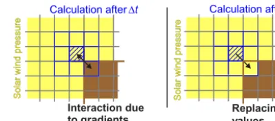
Figure 2.Density and pressure gradients across the planetary sur-face are related to forces if the MHD equations are solved within the entire simulation box. To minimize this interaction, the density and the pressure at the planetary surface are set to the values outside the planet.

of the plasma in the magnetosphere due to co-rotation of the plasma or magnetic reconnection, for example. Therefore, different from the simulation described by Ogino (1993), the simulation requires appropriate inner boundary conditions to allow a stable simulation for long time intervals. The plane-tary surface is approximated by a spherical surface with the distanceRPto the planet’s center. The distance of a grid point

(i, j, k)to the center is defined by

ri,j,k:= q

((i−iP) 1x)2+((j−jP) 1y)2+((k−kP) 1z)2. (16)

The velocity of the plasma inside the planet, i.e.,ri,j,k< RP, is

un_l,i,j,k=0, forri,j,k< RP, n=2,3,4. (17) It is also possible to set only the normal component of the velocity to zero.

Density and pressure gradients between the planet’s in-terior and the plasma outside must not cause forces on the plasma. However, the MHD equations are solved within the entire simulation domain. This can lead to an interaction as sketched in Fig. 2. The values at grid points inside the planet, which have at least one neighboring grid point outside, are replaced in every time step by average values of the sur-rounding neighboring grid points outside the planet, i.e., the non-boundary neighbors. Neighboring grid points of a grid point(iP, jP, kP)are{(iP±1, jP±1, kP±1)}. This procedure suppresses the interaction of density and pressure gradients across the planet.

in-duction equation simplifies to the diffusion equation

∂tB= −∇ ×

_η

µ0 ∇ ×B

. (18)

The resistivity distribution in the simulation box is modeled by

η=



 

 

ηCore, r < RCore

ηMantle, RCore≤r≤RP

ηA, otherwise

. (19)

Thereby, the planet’s interior consists of two regions with different resistivity, a core withηCore=1/σCoreand a mantle withηMantle=1/σMantle. The resistivity outside the planet is assumed to be constant withηA. As a consequence, the inter-action due to diffusion is allowed depending on the electrical resistivity of the planet. This is of particular importance if Mercury is considered; however, it is of minor importance for Earth.

2.3 Using spacecraft data

The simulation uses solar wind parameters as boundary con-ditions. With respect to the two spacecraft in mission Bepi-Colombo, simultaneous observations of the solar wind as well as the magnetic field close to the planet will be avail-able in the future. Thereby, the solar wind conditions can be determined either directly by in situ measurements or by us-ing the reconstruction method by Nabert et al. (2015) from data within the interaction region. This allows a precise de-termination with a high time resolution of the solar wind conditions. The THEMIS mission provides data from similar spacecraft constellations at Earth. The solar wind conditions observed by a spacecraft need to be transferred to the inflow boundary of the simulation box. Therefore, the solar wind data are shifted by1tSC/in, which is given by

1tSC/in=

nP·1rSC/in

nP·vSW

, (20)

where nP is the solar wind’s phase plane normal vector,

1rSC/in:=rSC−rinis the distance vector between the space-craft’s position rSC, with the center of the inflow boundary

rin.

For a comparison between simulation results and space-craft data, the data need to be transferred into MSP coordi-nates. Therefore, the THEMIS data are first transferred into geographic (GEO) coordinates. Vectors in these coordinates can be transferred into MSP coordinates by rotation matrices

Ry(θK)andRz(λK). These matrices are defined by

Ry(θK)=





cos(θK) 0 sin(θK)

0 1 0

−sin(θK) 0 cos(θK)



,

Rz(λK)=





cos(λK) −sin(λK) 0 sin(λK) cos(λK) 0

0 0 1



.

(21)

The rotation anglesθK andλK are determined by the solar wind velocity vector:

λK=

vy,SW,GEO

|vy,SW,GEO| arccos





vx,SW,GEO q

v2_x,SW,GEO+v_y,2_SW,GEO



,

θK= e

vz,SW,GEO

|

evz,SW,GEO| arccos



 e

vx,SW,GEO q

ev 2

x,SW,GEO+ev 2

z,SW,GEO 

.

(22)

Here, vSW,GEO=(vx,SW,GEO, vy,SW,GEO, vz,SW,GEO)T is the solar wind velocity vector using GEO coordinates and

evSW,GEOis defined by

evSW,GEO:= evx,SW,GEO,evy,SW,GEO,evz,SW,GEO T

:=Rz(λK)vSW,GEO.

Then, a vector in GEO coordinatesg_GEO can be transferred into a vector in MSP coordinatesg_MSPby

g_MSP=Ry(θK) Rz(λK)gGEO. (23)

Applying the coordinate transformation, the solar wind ve-locity becomes parallel to thexaxis.

For the validation of the code, the known planetary dipole moment components of Earth according to Table 1 with the normalization constant of Eq. (6) can be used:

mx= −0.051mnorm,

my= 0.158mnorm,

mz= −0.945mnorm.

(24)

To include the rotation of the planetary magnetic field due to the planet’s rotation, the magnetic moments of the mag-netic field are modified according to Eq. (23). The angles of the transformation will continuously vary along the space-craft’s trajectory. The rotation of the planetary magnetic field is performed every 200 time steps by subtracting the plan-etary field contribution from the total magnetic field at the time step considered and adding the planetary magnetic field corresponding to the new anglesθKandλK.

2.4 Validation of the simulation code

To validate the modified simulation code, we compare a sim-ulation using the known dipole moment of Earth according to Table 1 with THEMIS magnetosheath data from 24 Au-gust 2008 measured by THC (Angelopoulos, 2008). Solar wind conditions are observed by THB during the magne-tosheath transition. The size of the simulation box isxL= 50.0RE, yL=60.0RE, and zL=60.0RE, with the planet in the center. The simulation uses a grid with imax=200,

0 50

ρ

[cm ³]

0 200 400

vx

-100 -50 0 50

vy

-50 0 50

vz

0 0.5 1 1.5

p

[nPa]

-10 0 10

Bx

[nT]

-20

-100

10

By

[nT]

0:30 1:00 1:30 2:00 2:30 3:00 3:30 4:00 4:30

Bz

[nT]

UniversalWime

0 20 40 60 80

[km

s ]

-1

[km

s ]

-1

[km

s ]

-1

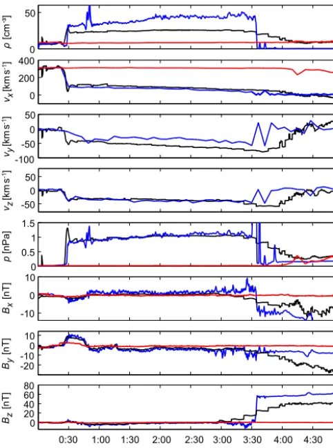
Figure 3. THC magnetosheath data (blue) observed on 24 Au-gust 2008 and the corresponding MHD simulation results (black) using the solar wind observations of THB (red).

simulation results on the spacecraft’s trajectory are presented in Fig. 3.

The bow shock is observed at about 00:30 UT and the magnetopause at about 03:30 UT in accordance with the sim-ulation results. Most physical quantities show a good agree-ment between actual observations and simulation results. Only the ion density in the magnetosheath is observed to be higher than in the simulation. Furthermore, the magnetic field in the magnetosphere is about 15 nT weaker than measured by the spacecraft. The magnetopause thickness is observed to be smaller than in the simulation, which is related to the diffusion coefficients required for a stable simulation. These differences between simulation result and data are mainly caused by numerical errors. This can impact an estimation of the planetary magnetic field. The lower magnetospheric mag-netic field will tend to overestimate the planetary magmag-netic field strength. However, this overestimation is limited due to the magnetopause location. A much stronger dipole mo-ment will increase the magnetopause distance and the mag-netic field will increase in the magnetosheath, which is not in accord with the observations. In general, the MHD sim-ulation results agree well with the observations made. In a

future step, the simulation code might be improved to reduce differences between simulation results and observations. An adaptive mesh refinement should be introduced to enhance the accuracy close to the magnetopause and reduce numeri-cal errors.

3 Data assimilation

3.1 Cost function and its minimization

In the previous section, spacecraft data were qualitatively compared to the results of the MHD simulation. To quantify the deviations, a cost function is introduced. Therefore, the method of least squares is used. The sum of squared resid-uals, FQ, ofMdata-measured valuesymat points xm with a

modelf depending on the parameterssis FQ:=

Mdata

X

m=1

(ym−f (xm,s))2. (25)

The parameterssof the MHD model are related to a vector spaceP. Here, for simplification, we consider only the plan-etary magnetic field parameters of the dipole and quadrupole. Thus, the parameters are

s=(m,Q)T=(mx, my, mz, Qxx, Qxy, Qxz, Qyy, Qyz)T, (26)

with Q:=(Qxx, Qxy, Qxz, Qyy, Qyz)T. The vector space

corresponding to these parameters is namedPD,Q. The pa-rameters of the modelsare estimated by minimizing the sum of squared residuals FQ. Transferred to the magnetic field ob-servationsBdata:=(Bx,data, By,data, Bz,data)Tand MHD sim-ulation resultsBsimu:=(Bx,simu, By,simu, Bz,simu)T with the spacecraft’s position in the orbitrSC,m, the cost functionK

is

K(s)=XMdata

m=1

Bx,data(rSC,m)−Bx,simu(rSC,m,s)

2

+ By,data(rSC,m)−By,simu(rSC,m,s)

2

+ Bz,data(rSC,m)−Bz,simu(rSC,m,s)

2 .

(27)

A gradient-based optimization can be used to minimize the cost function with respect to the parameters of the model

s. Starting from a point s0 in parameter space, new points

sk=(mk,Qk)Tare determined with everykth gradient

cal-culation. This optimization problem is without constraints and can be solved using a quasi-Newton method. We use the Broyden–Fletcher–Goldfarb–Shanno (BFGS) algorithm (Press et al., 1992) to minimize the cost function.

The algorithm requires the gradient of the cost functionK

with respect to the parameters of the model at pointssk in

parameter space. There are different possibilities to compute these gradients. For example, the gradient can be approxi-mated by difference quotients:

∂K(s) ∂s |s=sk ≈

NP X

l=1

K(sk+1slel)−K(sk)

1sl

where el denotes the lth unit vector and 1sl is the

corre-sponding step size in parameter spaceP. The sum of Eq. (28) includes all dimensions in parameter space(NP:=dim(P)).

Note that the gradient∂sK(s)is used as a column vector. The

step sizes1slneed to be adequately small to approximate the

gradient sufficiently well.

3.2 Automatic differentiation and adjoint method Each calculation of the cost function for a certain set of pa-rameters requires a full global MHD simulation of the data along the spacecraft’s trajectory. Thus,(NP+1)simulations

have to be performed in the calculation of the gradient ac-cording to Eq. (28). In general, the calculation is extremely time-consuming because of the nonlinearity of the MHD equations.

Another possibility to calculate the gradient∂sK(s)is the differentiation using analytical expressions, as explained in detail in the following. The solution of the MHD simulation depending on space and time coordinatesu(t,x)can be rep-resented by a vector ut,x on a numerical grid. This vector

contains the solution at all time steps and discrete positions in space for all physical quantities in its components. Thus, the number of components of the vectorut,xis

Nv=NvarNgridlmax, (29)

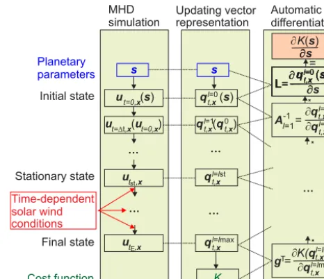
with the constants as defined in the previous chapter. The simulation code calculates the time- and spatially dependent solution of the MHD quantitiesu(t,x)iteratively. The iter-ation is implemented by a time loop in the simuliter-ation code, whereby u(t=l 1t,x)is computed from the results of the previous time stepu(t=(l−1) 1t,x)and the boundary con-ditions. Equivalently, the time iteration oflcan be considered as an iteration that steadily improves the approximation of the final solution vectorut,x , sketched in Fig. 4. Thereby,

after thelth iteration step, the vectorql

t,x contains the valid

solution for all time steps that satisfyt≤l 1t. The final so-lution qlmax

t,x =ut,x is obtained afterlmax iteration steps. At the 0th iteration step, the simulation needs to be initialized. The simulation code calculates the solution in thelth itera-tion step from the previous approximaitera-tion by a funcitera-tion F. Thus, thelth iteration step can be expressed by

ql_t,x(s)=F (ql_t,−1_x (s)) . (30) The cost functionK(qlmax

t,x (s))depends implicitly on the

pa-rameters s. With respect to the nested dependences of the solution in Eq. (30), the gradient of the cost function can be expressed by the chain rule:

∂K(qlmax

t,x (s))

∂s =

∂K(qlmax

t,x ) ∂qlmax

t,x

· ∂q

lmax

t,x ∂qlmax−1

t,x

·. . .

·∂q 1

t,x ∂q0_t,x

·∂q 0

t,x(s)

∂s .

(31)

Planetary parameters

u_t=0,x( )s

u_{t= ,Dtx}(u_t=0,x)

ql=0( )s t,x

ql=1(q )

t,x 0t,x

u_{t ,x}

u_{t ,x} s Initial state Stationary state Final state MHD simulation Time-dependent

solar wind

conditions

Cost function

ql l= st t,x

Updating vector

representation

ql l= max t,x

K

Automatic differentiation

ul=0( )s t,x

∂ ∂

L= u ( )s

l=0 t,x ∂ ∂ L= ∂ ∂ gT=

ql l= max t,x

K(ql l= max)

t,x

ul=0( )s t,x

∂ ∂

L= q ( )s

l=0 t,x ∂ ∂ L= ∂ ∂ A-1= _ql=0

t,x

ql=1 t,x l=1 s E st s ∂∂∂ ∂ ∂s

K( )s

=

Figure 4.The left column sketches the time iteration of the MHD simulation code starting from the initial state att=0 determined by the planetary magnetic field parameterss. At a certain time step, a stationary solutionust,xis obtained and time iteration continues us-ing time-dependent solar wind conditions until the simulation ends atutE,x. In the middle column, the corresponding interpretation of updating the complete time- and spatially dependent solution vector q_t,x is presented. The cost functionKis calculated from the final vector. On the right side, the automatic differentiation gradient cal-culation is presented, starting from the bottom and multiplying each factor according to Eq. (31).

This expression contains the stationary solution atl=lst be-cause 0< lst< lmax. Although the cost function is evaluated only after the stationary state has been obtained, i.e.l > lst, the cost function also depends implicitly on prior time steps because the stationary solution emerges from the initial state. The magnetic field components of the initial state vectoru0_t,x

depend on the parameterssbecause the initial magnetic field distribution in the simulation is created by the dipole and quadrupole parameters. Equation (31) can be written as

∂K(s)

∂s =g

T_·A−1

lmax·A −1

lmax−1·. . .·A −1

1 ·L (32)

using the following abbreviations: A−1_l := ∂q

l t,x ∂ql_t,−1_x , l

=1,2, . . ., lmax,

gT:=∂K(q

lmax

t,x ) ∂qlmax

t,x ,

L:=∂q 0

t,x(s) ∂s .

(33)

Therefore, the derivatives of the matrices in Eq. (31) can be determined by analytical expressions. The time iteration of the simulation code starts atl=0 and ends atlmax. After the

lth iteration step, the corresponding matrixA−1_l can be cal-culated. Starting from a unit matrix, the matrix containing the derivatives is multiplied after every time step to the left side. Finally, after lmaxiterations, the gradient∂K(s)/∂s is obtained.

This procedure is called forward differentiation because the gradient is calculated parallel to the execution of the time loop in the simulation code. The advantage over the compu-tation of the gradient using difference quotients according to Eq. (28) is that no errors due to finite step sizes occur. For-ward differentiation can be applied by hand to the simulation code, or alternatively, by an automatic differentiation (AD) tool (Wengert, 1964). Therefore, the cost functionKand its dependent parameterssneed to be declared in the code. The AD tool identifies all implicit dependences. The required an-alytical expressions for the derivations are taken from a li-brary of the AD tool and inserted at the correct positions in the code. Note that the library contains elementary analytical derivations of all important expressions such as∂xsin(x)=

cos(x). According to Eq. (31), the inserted expressions are related to each other such that the required gradient is com-puted. Several different AD tools were developed during the last decades. Here, the Transformation of Algorithms in For-tran (TAF) tool (Giering and Kaminski, 2003) from the com-pany FastOpt was used (http://www.FastOpt.com).

An AD tool is able to differentiate a numerical code au-tomatically, i.e., the tool can be applied without considering details of the implementation. However, for complex numer-ical codes, such as MHD simulation codes, problems might occur. For example, codes using parallel computing function calls by the message-passing interface (MPI), as they are also used for our simulation code, usually need further treatment. The analytical forward differentiation with an AD tool is also called automatic forward differentiation.

The computational costs for the calculation of the gradient with difference quotients or using automatic forward differ-entiation do not differ much. However, the latter procedure leads to a more efficient approach, the adjoint method. The adjoint method is extensively used for optimization problems in fluid dynamics, e.g., drag minimization by variations in surface geometry (e.g., Jameson, 1988; Othmer, 2008, 2014; Meader and Martins, 2012) or in seismology (e.g., Fichtner et al., 2006).

The adjoint method can be introduced with systems of linear equations, as described briefly in the following (e.g., Giles and Pierce, 2000; McNamara et al., 2004; Nabert et al., 2015). The symbols used for variables, vectors, and matri-ces refer to the previous considerations and will be marked by an asterisk as an index for distinction. We consider the following system of equations

A∗·X∗=L∗, (34)

with the matrices of the coefficientsA∗, the solutionX∗, and the inhomogeneityL∗. All elements of the matrices are real numbers. The scalar product of a vectorg_∗with the matrix X∗should be calculated using the following equation:

gT∗·X∗=?. (35)

This scalar product can be computed by solving Eq. (34) first, and then calculating the product of vectorg∗ with the solu-tionX∗. This approach is called forward calculation.

Another possibility is to use the adjoint method. To deduce the method, the product of a vectoryTwith both sides of the system of linear Eq. (34) is considered:

yT_∗·A∗·X∗=yT_∗·L∗. (36)

The vectory∗is defined by

yT_∗·A∗=gT_∗. (37)

This equation is transposed, which leads to the adjoint system of equations

AT_∗y∗=g∗. (38)

Using Eqs. (36) and (37), the scalar product (Eq. 35) can be written as

gT_∗·X∗=yT_∗·A∗·X∗=yT_∗·L∗. (39) If the adjoint system of Eq. (38) is solved,yT

∗·L∗can be com-puted, which is nothing other than the scalar product (Eq. 35) as seen in Eq. (39).

The computational costs are mainly determined by the number of multiplications and differ for both possibilities of calculating the scalar product (Eq. 35). Only in case of a column vector inhomogeneityL∗, is the number of multi-plications equal. If the matrixL∗ consists ofN∗,P column

vectors,N∗,P systems of linear equations with a vector

in-homogeneity need to be solved in the forward calculation. The adjoint method is independent ofN∗,Pand only a single

system of linear equations needs to be solved. Therefore, the latter approach requiresN∗,P times fewer multiplications.

The adjoint approach can be applied to the calculation of the gradient in Eq. (32). If the product of all matricesA−1:= A−1_l

max·. . .·A −1

1 in Eq. (32) is substituted, this leads to

∂K(s)

∂s =g

T_·A−1_{·L. (40)}

The second product on the right side of Eq. (40) can be sub-stituted by

X:=A−1·L. (41)

During the analytical forward differentiation, the gradient is computed successively using chain rule from the right to the left. This corresponds to a procedure, where, at first, the system of linear Eq. (34) is solved with respect to X∗ and then, the scalar product (Eq. 35) is calculated. If the matrix products of Eq. (40) are computed from left to right, at first, the product

yT:=gT·A−1 (42)

is determined. This corresponds to solving the adjoint Eq. (38) with respect toy_∗. The scalar product (Eq. 35) is determined byyT

∗·L∗, which is related to the multiplication of yT_{·Lto determine the cost function. Thus, the adjoint} method for the gradient calculation of the cost function can be identified with the execution of the multiplications from the left to the right in Eq. (40).

The dimensions of the vectors and matrices involved are dim(g)=Nv×1, dim(L)=Nv×NP, and dim(A)=Nv×

Nv. The calculation of the gradient by computing the matri-ces from the right to the left in Eq. (40) requiresNrl multipli-cations of components, whereby

Nrl=Nv2NP(Nv+1) . (43)

If the gradient is calculated from the left to the right in Eq. (40),Nlrmultiplications of components are performed:

Nlr=Nv2(Nv+NP) . (44)

The limit NP=1 leads to Nrl=Nlr. Usually, one can as-sumeNPNvbecause the number of grid points exceeds the dimensions of parameter space, which is eight for the dipole and quadrupole parameters. Then, Eq. (44) simplifies to

Nlr=NrlNP. (45)

Thus, the multiplication of the matrices in Eq. (40) from the left to the right, the adjoint approach, is more efficient for many parameters and requires aboutNP times fewer

multi-plications. The evaluation procedure for the simulation code is depicted in Fig. 4.

However, the numerical implementation of the adjoint method is more difficult than the analytical forward differ-entiation. As described, the calculation of the gradient with the analytical forward differentiation is parallel to the exe-cution of the time loop in the simulation code. In contrast, the solution at the last time iterationqlmax

t,x has to be known to

calculategT·A−1_l

max. Thus, at first, the simulation needs to be performed once, whereby all calculation results that are re-quired for the matrix multiplications are stored temporarily. Then, the gradient can be computed according to the adjoint approach.

There are AD tools that can derive codes not only accord-ing to forward differentiation but also accordaccord-ing to the ad-joint method. However, the available memory on a computer

is often too small to store all the required results in the cen-tral memory. The memory consumptionMMemorycan be es-timated by multiplying the number of grid points of the sim-ulation boxNgridaccording to Eq. (14) with the number of time stepslmax, the number of MHD variablesNvar, and the size of a MHD variableMvar:

MMemory≈NgridlmaxNvarMvar. (46) The number of variables of the MHD simulation isNvar=8 and the size of such a variable isMvar=4 bytes if a float variable is assumed. This gives a memory consumption of about 1600 GB for a simulation grid imax=jmax=kmax= 100 andlmax=5×105. The central memory is often much smaller, so that a certain portion of the variables needs to be stored on the hard disk. However, the seek time of the central memory is much smaller, and thus, the runtime of the algorithm becomes longer by storing data on the hard disk.

To minimize the access to the hard disk, checkpointing can be used. Thereby, the main iteration loop of the algo-rithm is split at certain checkpoints into smaller loops. Then, the smaller loop iterates overNloop,checkiterations instead of the complete time loop withlmaxiterations. This reduces the memory requirements for such a loop to

MMemory,check=

Nloop,check

lmax

MMemory. (47)

The variables during a calculation of such a smaller loop can be stored within the central memory. After the execu-tion of the smaller loop, the results are stored to the hard disk to combine all results of the smaller loop. However, using smaller loops, the adjoint method can only be applied within these smaller loops. Thus, checkpointing reduces the seek time of the memory, but the adjoint approach is restricted to a smaller part of the algorithm. In total, this reduces the runtime of the algorithm, but the performance is below the theoretical possible performance of the adjoint approach with unlimited central memory space.

Note that instead of using only observations of a single spacecraft, simultaneous measurements from multiple space-craft at different locations can be calculated in Eq. (27) as well. This can be done without additional computational costs and memory capacity because the solution of the MHD simulation is calculated in the entire simulation domain and stored anyway.

3.3 Adjoint MHD simulation code

0.7 0.8 0.9 1.0 1.1 1.2 m /z

10-8 10-6

10-4 10-2

R

el

. e

rr

or

mx

my

mz

250 500 750 1000 1250 1500

Iteration

mx

my

mz 10-8

10-6

10-4 10-2

R

el

. e

rr

or

mnorm

Figure 5.The relative errors for gradients determined by difference quotients and the adjoint method for the dipole components. Thereby, on the left side, different points in parameter space are considered. On the right side, the dependence of the error on a different number of time iteration steps is shown.

250 500 750 1000 1250 1500 0.62

0.64 0.66 0.68 0.70

tAdj

/

tDQ

Iteration 250 500 750 1000 1250 1500

0.5 1.0 1.5 2.0 2.5 104

Iteration

Runtime [s]

tAdj tDQ

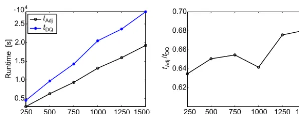
Figure 6. The runtime of calculating gradients using the adjoint methodtAdj and using difference quotientstDQ. On the left side, the dependence on the number of time iteration steps is presented. On the right side, the ratio of the runtimes is shown.

considered. Thus, the adjoint code computes the gradient of the cost function (27) with respect to the parameters (26).

To validate the adjoint MHD simulation code, the gradi-ents produced by the adjoint code are compared to those calculated by difference quotients according to Eq. (28). Therefore, at first, the interaction of the solar wind with the planetary magnetic field is neglected and the planetary magnetic field represented by its dipole and quadrupole mo-ments is only taken into account. Gradients at certain points

s0=(0,0, mz,0,0,0,0,0)T in parameter space are

consid-ered. Thereby, the mz component varies between 0.7 and

1.2mnorm with a step size of 0.1mnorm. The spacecraft data

Bdataon a trajectoryrSC, required to calculate the cost func-tion, are generated synthetically along the x axis between 20.2 and 9REwith a step size of 0.42RE. The gradient of the cost function is calculated using difference quotients∂s₀KDQ and the adjoint method∂s₀KAdjfor differents0. The relative error of theith component of the gradient is defined by

rel. error:= ∂s0KDQ

−∂s₀KAdj

·ei

max(∂s₀KDQ·ei, ∂s0KAdj·ei)

. (48)

Here, The result of the maximum function max(a, b)is the larger value ofa andbandei defines theiunit vector. The

relative error of the dipole moment for differents0is depicted in Fig. 5. The error is smaller than 10−4, i.e., both gradients agree for different values ofmz.

Now, the interaction of the planet with the solar wind is taken into account. Thereby, the gradients calculated by the adjoint method can be compared to gradients computed by difference quotients for a different number of time iterations. The corresponding relative errors of the dipole components of the gradient are shown in Fig. 5 on the right side. It is seen that the gradients agree very well.

5 10 15 20 Iteration

mx my mz

-0.2 0.0 0.2 0.4 0.6 0.8 1.0 1.2

Moments

/

mnorm

5 10 15 20 25 30

Iteration

mx my mz

-0.2 0.0 0.2 0.4 0.6 0.8 1.0 1.2

Moments

/

mnorm

5 10 15 20 25 30 35 40 Iteration

mx mz Qxy

-0.2 0.0 0.2 0.4 0.6 0.8 1.0 1.2

Moments

/

mnorm

5 10 15 20 25 30 35

Iteration

mx mz Qxy

-0.2 0.0 0.2 0.4 0.6 0.8 1.0 1.2

Moments

/

mnorm

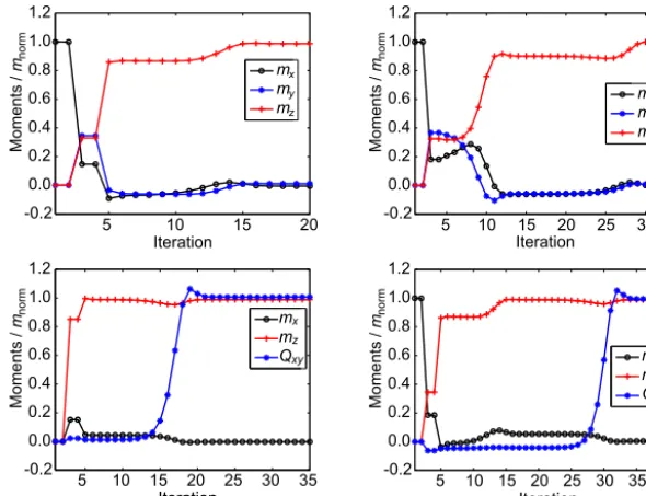
Figure 7.Estimation of planetary moments neglecting the interaction with the solar wind and using synthetic data. The reconstructions shown in the upper panels take only a dipole moment into account. These two results consider a different spacecraft trajectory, with a trajectory closer to the planet corresponding to the left figure. All reconstructions presented use the same dipole moment for calculating the synthetic spacecraft data. However, in the lower panels, an additional quadrupole component was introduced. The reconstructions in the lower panels use a different choice of the initial parameters for the estimation.

the middle. Using these results, the automatic differentiation procedure calculates the gradient as sketched on the right from bottom to top, which corresponds to another simulation run. Thus, in theory, the adjoint method can be up to 78 % faster than the difference quotient calculation. However, our adjoint code uses checkpointing because the central memory is too small, which increases the runtime.

Consequently, the test computer configuration is not opti-mal to achieve the best performance. The performance can be improved by using a computer cluster with distributed mem-ory space. Then, each core can access its own memmem-ory space and checkpointing can be avoided. This can increase the per-formance. Furthermore, it should be noted that without addi-tional computaaddi-tional costs and memory requirements, more parameters can be introduced in the estimation process of the adjoint approach, such as octupole planetary magnetic field parameters.

4 Estimation of planetary magnetic field parameters 4.1 Using synthetic data

At first, the results of data assimilation using synthetically produced data are considered, neglecting the interaction of the planetary magnetic field. The simulation box has a length of 60.2RE in every dimension with the planet in its center. The number of grid points isimax=jmax=kmax=300. Syn-thetic spacecraft dataBdataare calculated from the magnetic

field distributions of certain dipole and quadrupole param-eterssPlanet along a trajectory rSC(x). The initialization s0 for the estimation procedure of the planetary parameters dif-fer from these moments. Starting from this initialization, the cost function is minimized.

The first trajectory considered here is rSC(x)=

(x,10.1RE−x,0)T, which is diagonal within the

xy plane. The spacecraft’s magnetic field data Bdata are generated by a dipole along the z axis, i.e.,

sPlanet=(0,0,1,0,0,0,0,0)Tmnorm. In parameter space, the starting point of the estimation procedure is

s0=(1,0,0,0,0,0,0,0)Tmnorm, which is nothing other than a dipole along the x axis. The BFGS algorithm it-eratively computes new gradients in which direction the cost function (27) is minimized. The corresponding dipole parameters during the minimization, depending on the iteration step of calculating new gradients, are presented in Fig. 7 in the top left panel. The vector of the dipole moment

-20 -100 10

Bx

[nT]

-20 -100 10

By

[nT]

0:30 1:00 1:30 2:00 2:30 3:00 3:30 4:00 4:30 0

20 40 60 Bz

[nT]

Universal time

1 3 5 7 9 11 13 Iteration

K

25 30 35 40 45

1 3 5 7 9 11 13 -1.2

-1.0 -0.8 -0.6 -0.4 -0.20.0 0.2 0.4

Iteration

mx

my

mz

Dipole

moment

/ m

norm

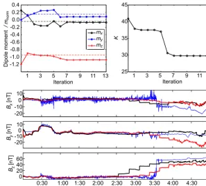
Figure 8.Estimation of Earth’s dipole moment from magnetosheath data of THC on 24 August 2008 using the THB solar wind observations, which are presented in Fig. 3. The variations in the dipole moment during the iteration process (top left) and the corresponding values of the cost function (top right) are shown. The values of the dipole moment of Earth are sketched as dashed lines. The plot on the bottom shows the iterative assimilation of the MHD simulation to the THC data (blue) before the first iteration (black) and after the 13th iteration (red).

The simultaneous estimation of dipole and quadrupole pa-rameters is considered as well by using magnetic field data

Bdata generated by sPlanet=(0,0,1,1,0,0,0,0)Tmnorm. Thereby, the trajectory rSC(x)=(x,10.1RE−x,0)T is used. The reconstruction of the planetary magnetic field, starting from s0=(0,0,0,0,0,0,0,0)Tmnorm, is shown in Fig. 7 in the bottom left panel. Additionally, the estima-tion process from a different point in parameter space s0=

(1,0,0,0,0,0,0,0)Tmnorm is realized. The results are pre-sented in Fig. 7 in the bottom right panel. In both situations, the momentssPlanet were correctly determined. Thereby, the estimation starting in parameter space farther away from the solution required 15 more iteration steps. Altogether, it is seen that the dipole as well as the quadrupole parameters can be reconstructed from synthetic data, whereby larger mag-netic field variations along the trajectory or a starting point

s0closer to the minimum speed up the estimation process. 4.2 Using THEMIS data

After proving the general functionality of the algorithm, it is applied using THEMIS spacecraft data at Earth. Thereby, data from the magnetosheath, a region strongly influenced by the interaction process of the solar wind, is considered. Different to the situation at Earth, spacecraft magnetic field observations in Mercury’s magnetosphere are strongly

mod-ified due to the magnetosphere’s small size. Here, we re-strict our approach to Earth’s magnetosheath data to con-sider a strongly disturbed magnetic environment compara-ble to the situation at Mercury. However, in final applica-tion, magnetospheric data will be used as well to reduce errors. Due to the weak components of the quadrupole at Earth, their influence is negligible close to the magnetopause. The largest quadrupole moment corresponds to a magnetic field of <0.1 nT at 10RE. This is very small compared to the contribution of the dipole’s z component of about 30 nT. Thus, only the dipole moment is considered in the es-timation at Earth. The eses-timation process starts froms0=

(0.25,0,−1.2,0,0,0,0,0)Tmnormin parameter space. Sub-sequently, the cost function is minimized iteratively, whereby every new calculation of a gradient denotes a new iteration step.

and 6 to 7. After the eighth iteration step, the cost func-tion and the components of the dipole moment do not change much. Finally, the solution vector after 13 iteration steps is s13=(−0.072,0.084,−1.078,0,0,0,0,0)Tmnorm. Thereby, all components are closer to the value of the dipole moment of Earth according to Eq. (24) than the initial val-ues. The relative errors for the dipole components are1mx=

(s13,1−mx,E)/mx,E= −0.44,1my=(s13,2−my,E)/my,E= −0.47, and1mz=(s13,3−mz,E)/mz,E=0.14. The relative error of the z component is the smallest because Earth’s dipole is mainly along thezdirection. Considering the mag-nitude, the relative error is 0.13. The panels showingBx,By,

andBzin Fig. 8 show the magnetic field distribution of the

MHD simulation, which corresponds tos0ands13.

5 Conclusions

We introduced an approach to estimating planetary parame-ters using global MHD simulations of the interaction of the solar wind with a planet. A simple MHD simulation code was introduced and prepared for an automatic differentiation tool to obtain an adjoint MHD simulation code. The differ-ences of spacecraft data and corresponding simulation results are quantified by a cost function, which is minimized by a gradient-based optimization. The adjoint code computes the gradient with lower computational effort compared to a dif-ference quotient calculation.

Our approach is designed to estimate planetary magnetic fields, especially if the field strength is weak so that the inter-action strongly modifies the magnetic field of the planet’s en-vironment. We used THEMIS data of Earth’s magnetosheath to simulate such an environment to test our approach. The results of the estimation process can be affected by statisti-cal and systematic errors. Therefore, statististatisti-cal errors will not contribute to the mean values of the estimated planetary mag-netic field if a sufficiently large number of magnetosheath transitions are considered. For example, the solar wind den-sity can be measured incorrectly due to a spacecraft poten-tial (McFadden et al., 2008). However, the density is usu-ally equusu-ally overestimated and underestimated. Considering a single magnetosheath transition, the estimated dipole mag-nitude of Earth differs about 13 % from the expected value. Based on this approach, further transitions can be considered to minimize the errors. Note that including magnetospheric data at Mercury will further reduce the statistical error. The runtime of the parameter estimation using the test computer is about 1 week using the 5 h magnetosheath data. This fast calculation procedure allows taking a lot more data into ac-count, especially if supercomputers are used.

We used a simple MHD simulation code to investigate the automatic differentiation procedure. As a next step, the sim-ulation code needs to be improved, e.g., by an adaptive mesh refinement, to reduce numerical errors. Also, kinetic or hy-brid simulation codes can be considered and treated with an

automatic differentiation tool. The limiting factor for apply-ing the automatic differentiation is not the complexity of the code but the memory consumption. Using our test computer, the adjoint approach was about 33 % faster than a finite dif-ference approach. Although the adjoint MHD code does not calculate the gradient very much faster than using difference quotients, it has the advantage that further parameters such as higher-order magnetic field moments or parameters of the planet’s conductivity can be included with nearly no addi-tional computaaddi-tional costs. Nonetheless, the performance of the adjoint code is, related to memory limitations of our test computer, much lower than expected from theory. Thus, as a further step, the test computer configuration needs to be mod-ified to increase performance. It is beneficial for the adjoint approach that each core has access to its own memory, which is different from our test computer. Thus, instead of using traditional supercomputers with fewer more powerful puters, a computer cluster using many commoditized com-puters with their own memory should be considered. These computer configurations recently became very popular in big data analysis using Google’s well-known MapReduce tech-nique (Dean and Ghemawat, 2004). A similar configuration might be more suitable for the adjoint code and increase its performance. The ability of our approach to perform on clus-ters with many cores depends on the parallelization of the MHD simulation code. Although this can be limited to a cer-tain number of cores, another possibility to parallelize the es-timation process is to split the data into subsets and perform the calculation of these subsets in parallel. Each data set will provide an individual estimator of the planetary parameters that can be applied in an ensemble averaging technique to reduce errors.

Data availability. Data from the THEMIS mission are publicly available and can be obtained from http://themis.ssl.berkeley.edu/ data/themis from the University of California Berkeley (Angelopou-los, 2008).

Competing interests. The authors declare that they have no conflict of interest.

Acknowledgements. This work is financially supported by the Ger-man Ministerium für Wirtschaft und Energie and the GerGer-man DLR under grants 50OC1403 and 50QW1501. We acknowledge NASA contract NAS5-02099 and V. Angelopoulos for use of data from the THEMIS mission. We specifically thank C. W. Carlson and J. P. Mc-Fadden for use of ESA data. We thank T. Ogino and K. Fukazawa for providing a version of their MHD simulation code. Furthermore, we thank FastOpt (R. Giering and T. Kaminski) for applying their TAF tool for the automatic differentiation procedure.

References

Alexeev, I. I., Belenkaya, E. S., Slavin, J. A., Korth, H., Anderson, B. J., Baker, D. N., Boardsen, S. A., Johnson, C. L., Purucker, M. E., Sarantos, M., and Solomon, S. C.: Mercury’s magneto-spheric magnetic field after the first two MESSENGER flybys, Icarus, 209, 23–39, doi:10.1016/j.icarus.2010.01.024, 2010. Angelopoulos, V.: The THEMIS Mission, Space Sci. Rev., 141, 5–

34, doi:10.1007/s11214-008-9336-1, 2008.

Benkhoff, J., van Casteren, J., Hayakawa, H., Fujimoto, M., Laakso, H., Novara, M., Ferri, P., Middleton, H. R., and Ziethe, R.: BepiColombo – Comprehensive exploration of Mercury: Mis-sion overview and science goals, Planet. Space Sci., 58, 2–20, doi:10.1016/j.pss.2009.09.020, 2010.

Clauser, C.: Einführung in die Geophysik, Springer Spektrum, Berlin Heidelberg, 2016.

Dean, J. and Ghemawat, S.: MapReduce: Simplified data processing on large clusters, in: Proceedings of Operating Systems Design and Implementation, 137–150, San Francisco, 2004.

Fichtner, A., Bunge, H.-P., and Igel, H.: The adjoint method in seismology: I – Theory, Phys. Earth Planet. In., 157, 86–104, doi:10.1016/j.pepi.2006.03.016, 2006.

Finlay, C. C., Maus, S., Beggan, C. D., Bondar, T. N., Chambodut, A., Chernova, T. A., Chulliat, A., Golovkov, V. P., Hamilton, B., Hamoudi, M., Holme, R., Hulot, G., Kuang, W., Langlais, B., Lesur, V., Lowes, F. J., Lühr, H., MacMillan, S., Mandea, M., McLean, S., Manoj, C., Menvielle, M., Michaelis, I., Olsen, N., Rauberg, J., Rother, M., Sabaka, T. J., Tangborn, A., Tøffner-Clausen, L., Thébault, E., Thomson, A. W. P., Wardinski, I., Wei, Z., and Zvereva, T. I.: International Geomagnetic Reference Field: the eleventh generation, Geophys. J. Int., 183, 1216–1230, doi:10.1111/j.1365-246X.2010.04804.x, 2010.

Gauss, C. F.: Allgemeine Theorie des Erdmagnetismus, in: Resul-tate aus den Beobachtungen des Magnetischen Vereins im Jahre 1838, edited by: Gauss, C. F. and Weber, W., 1–59, Göttinger Magnetischer Verein, Leipzig, 1839.

Giering, R. and Kaminski, T.: Applying TAF to generate efficient derivative code of Fortran 77–95 programs, Proceedings in Ap-plied Mathematics and Mechanics, 2, 54–57, 2003.

Giles, M. B. and Pierce, N. A.: An Introduction to the Adjoint Approach to Design, Flow Turbul. Combust., 65, 393–415, doi:10.1007/s11214-008-9365-9, 2000.

Glassmeier, K.-H.: Currents in Mercury’s Magnetosphere, in: Mag-netospheric Current Systems, Geophysical Monograph 118, 371–380, American Geophysical Union, Washington DC, 2000. Glassmeier, K.-H. and Tsurutani, B. T.: Carl Friedrich Gauss – Gen-eral Theory of Terrestrial Magnetism – a revised translation of the German text, History of Geo- and Space Sciences, 5, 11–62, doi:10.5194/hgss-5-11-2014, 2014.

Glassmeier, K.-H., Grosser, J., Auster, U., Constantinescu, D., Narita, Y., and Stellmach, S.: Electromagnetic Induction Effects and Dynamo Action in the Hermean System, Space Sci. Rev., 132, 511–527, doi:10.1007/s11214-007-9244-9, 2007.

Grosser, J., Glassmeier, K.-H., and Stadelmann, A.: Induced mag-netic field effects at planet Mercury, Planet. Space Sci., 52, 1251– 1260, doi:10.1016/j.pss.2004.08.005, 2004.

Heyner, D., Wicht, J., Gómez-Pérez, N., Schmitt, D., Auster, H.-U., and Glassmeier, K.-H.: Evidence from Numerical Experiments for a Feedback Dynamo Generating Mercury’s Magnetic Field, Science, 334, 1690–1693, doi:10.1126/science.1207290, 2011.

Jameson, A.: Aerodynamic Design via Control Theory, J. Sci. Com-put., 3, 233–260, doi:10.1007/BF01061285, 1988.

Jia, X., Slavin, J. A., Gombosi, T. I., Daldorff, L. K. S., Toth, G., and Holst, B.: Global MHD simulations of Mercury’s magne-tosphere with coupled planetary interior: Induction effect of the planetary conducting core on the global interaction, J. Geophys. Res.-Space, 120, 4763–4775, doi:10.1002/2015JA021143, 2015. Johnson, C. L., Purucker, M. E., Korth, H., Anderson, B. J., Winslow, R. M., Al Asad, M. M. H., Slavin, J. A., Alexeev, I. I., Phillips, R. J., Zuber, M. T., and Solomon, S. C.: MESSENGER observations of Mercury’s magnetic field structure, J. Geophys. Res.-Planet., 117, E00L14, doi:10.1029/2012JE004217, 2012. Korth, H., J. Anderson, B., Acuña, M. H., Slavin, J. A.,

Tsy-ganenko, N. A., Solomon, S. C., and McNutt, R. L.: De-termination of the properties of Mercury’s magnetic field by the MESSENGER mission, Planet. Space Sci., 52, 733–746, doi:10.1016/j.pss.2003.12.008, 2004.

Langel, R. A.: The main field, in: Geomagnetism, edited by: Jacobs, J. A., 249–512, Academic Press, London, 1987.

Lax, P. and Wendroff, B.: Systems of conservation laws, Commun. Pur. Appl. Math., 13, 217–237, doi:10.1002/cpa.3160130205, 1960.

McFadden, J. P., Carlson, C. W., Larson, D., Ludlam, M., Abiad, R., Elliott, B., Turin, P., Marckwordt, M., and Angelopoulos, V.: The THEMIS ESA Plasma Instrument and In-flight Calibration, Space Sci. Rev., 141, 277–302, doi:10.1007/s11214-008-9440-2, 2008.

McNamara, A., Treuille, A., Popovi´c, Z., and Stam, J.: Fluid Con-trol Using the Adjoint Method, ACM T. Graphic., 23, 449–456, doi:10.1145/1015706.1015744, 2004.

Meader, C. A. and Martins, J. R. R. A.: Derivatives for Time-Spectral Computational Fluid Dynamics Using an Au-tomatic Differentiation Adjoint, The American Institute of Aeronautics and Astronautics Journal, 50, 2809–2819, doi:10.2514/1.J051658, 2012.

Nabert, C., Glassmeier, K.-H., and Plaschke, F.: A new method for solving the MHD equations in the magnetosheath, Ann. Geo-phys., 31, 419–437, doi:10.5194/angeo-31-419-2013, 2013. Nabert, C., Othmer, C., and Glassmeier, K.-H.: Solar wind

recon-struction from magnetosheath data using an adjoint approach, Ann. Geophys., 33, 1513–1524, doi:10.5194/angeo-33-1513-2015, 2015.

Ogino, T.: A three-dimensional MHD simulation of the interaction of the solar wind with the earth’s magnetosphere – The genera-tion of field-aligned currents, J. Geophys. Res., 91, 6791–6806, doi:10.1029/JA091iA06p06791, 1986.

Ogino, T.: Two-Dimensional MHD Code, in: Computer Space Plasma Physics: Simulation Techniques and Software, edited by: Matsumoto, H. and Omura, Y., 161–207, Terra Scientific Pub-lishing Company, Tokyo, 1993.

Ogino, T., Walker, R. J., Ashour-Abdalla, M., and Dawson, J. M.: An MHD simulation of By-dependent magnetospheric convec-tion and field-aligned currents during northward IMF, J. Geo-phys. Res., 90, 10835–10842, doi:10.1029/JA090iA11p10835, 1985.

Othmer, C.: Adjoint methods for car aerodynamics, Journal of Mathematics in Industry, 4, 6, doi:10.1186/2190-5983-4-6, 2014. Press, W. H., Teukolsky, S. A., Vetterling, W. T., and Flannery, B. P.: Numerical recipes in FORTRAN, Cambridge University Press, Cambridge, 1992.

Solomon, S. C., McNutt, R. L., Gold, R. E., Acuña, M. H., Baker, D. N., Boynton, W. V., Chapman, C. R., Cheng, A. F., Gloeck-ler, G., Head, III, J. W., Krimigis, S. M., McClintock, W. E., Murchie, S. L., Peale, S. J., Phillips, R. J., Robinson, M. S., Slavin, J. A., Smith, D. E., Strom, R. G., Trombka, J. I., and Zu-ber, M. T.: The MESSENGER mission to Mercury: scientific ob-jectives and implementation, Planet. Space Sci., 49, 1445–1465, doi:10.1016/S0032-0633(01)00085-X, 2001.

Stadelmann, A., Vogt, J., Glassmeier, K.-H., Kallenrode, M.-B., and Voigt, G.-H.: Cosmic ray and solar energetic particle flux in paleomagnetospheres, Earth Planets Space, 62, 333–345, doi:10.5047/eps.2009.10.002, 2010.

Vogt, J. and Glassmeier, K. H.: On the location of trapped parti-cle populations in quadrupole magnetospheres, J. Geophys. Res., 105, 13063–13072, doi:10.1029/2000JA900006, 2000.

Wengert, R. E.: A simple automatic derivative evaluation program, Commun. ACM, 7, 463–464, 1964.