Output feedback model reference adaptive control for multi-input–multi-output plants with state delay

www.elsevier.com/locate/sysconle

Output feedback model reference adaptive control for

multi-input–multi-output plants with state delay

Boris M. Mirkin

, Per-Olof Gutman

Faculty of Civil and Environmental Engineering, The Division of Environmental, Water, and Agricultural Engineering, Technion, Israel Institute of Technology, Haifa 32000, Israel

Received 5 August 2003; received in revised form 14 October 2004; accepted 14 February 2005 Available online 2 April 2005

Abstract

Two new output feedback adaptive control schemes based on Model Reference Adaptive Control (MRAC) and adaptive laws for updating the controller parameters are developed for a class of linear multi-input–multi-output (MIMO) systems with state delay. An effective controller structure established on a new error equation parametrization is proposed to achieve tracking with the error tending to zero asymptotically. To achieve exact asymptotical tracking, we introduce, in the standard MRAC structure for plants without delay, a new additional adaptive feedforward control component as an output of a dynamical system driven by the reference signal. Adaptive laws are developed using the SPR-Lyapunov design approach and two assumptions regarding the prior knowledge of the high-frequency matrixK_p. This work is the first asymptotic exact zero tracking results for this class of systems in the framework of the certainty equivalence approach.

© 2005 Elsevier B.V. All rights reserved.

Keywords: Model reference adaptive control; Multi-input–multi-output (MIMO) state-delay systems; SPR-Lyapunov design; Output

feedback; Stability

1. Introduction

Many physical systems can be modeled by delay differential equations. In these models, time delays are often used to represent the effect of e.g. transmis-sion, and transportation. Often time delays can be used as an approximation of complex models. Much effort has been devoted to providing a theory for the

con-∗_{Corresponding author. Tel.: +97 248 292629; fax:} +97 248 221529.

E-mail address:[email protected](B.M. Mirkin).

0167-6911/$ - see front matter © 2005 Elsevier B.V. All rights reserved. doi:10.1016/j.sysconle.2005.02.008

controllers guarantee that all closed-loop solutions converge to some bounded residual set. An adaptive discontinuous output feedback controller was consid-ered in [16] to achieve exact asymptotic regulation for a class of single-input, single-output systems de-scribed by nonlinear functional differential equations. See also the recent paper for the multi-input–multi-output (MIMO) case [7]. Subsequently, adaptive tracking control was considered for the same class of systems in [17], using a continuous feedback on one hand, and discontinuous feedback on the other hand. Using continuous feedback[17], achieved only practical tracking, i.e. convergence to some bounded residual set. Discontinuous feedback enabled [17], as well as[1] to achieve exact asymptotic tracking, i.e. in the sense that the tracking error asymptoti-cally approaches zero. State feedback Model Refer-ence Adaptive Control (MRAC) was investigated in [19,10].

Recently a new approach [11,12] was developed for the output model reference adaptive control of single-input (u(t)∈ R) single-output (y(t)∈ R) lin-ear continuous-time plants with state delay described by equations, suitably initialized, of the form

˙

x(t)=Ax(t)+Ax(t−)+bu(t), y(t)=cTx(t)

with unknown A,A, b and c of appropriate dimen-sions and known time delay. The main idea is to treat the state delay element not as a part of the plant but rather as the input to the systemW0(s)=cT(Is−A)−1b

and then decompose the control law into two compo-nents. The first base component is designed by a stan-dard MRAC procedure[18,14,8]as for a plant without delayW0(s)but applied to the time-delay plant. The second component is formed by a special adaptively adjusted dynamic system P(s,ff)as a function of the reference signalr(t). This makes it possible to use the well-understood MRAC design technique.

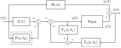
In the framework of the standard MRAC control structure, which is widely used in the control literature for plants without delay, e.g.[18, p. 104]our adaptive controller can be represented by the scheme inFig. 1. From Fig. 1 it is clear that in the feedback path e=y −yr is used instead of y. In addition to the standard memoryless feedforward block withr(t)as the input and with the adjustable gain_r(t), there is a prefilterP (s,ff)also withr(t)as the input, with the

Fig. 1. Adaptive control structure with the auxiliary dynamic feed-forwardP (s,ff).

adjustable vector gain ff. The special choice of the

adaptive prefilter structure makes it possible to solve the problem of adaptive exact asymptotic output track-ing under parametric uncertainties for a delay system. In [11,12], it was shown how the prefilter can be de-signed.

The main contribution of the present paper is the design of a new adaptive control scheme which gen-eralizes the results in[12]as follows:1

(i) the class of systems is enlarged to a class of multi-input u(t)∈ Rm multi-output y(t)∈ Rm systems.

(ii) we construct two different types of prefilters P (s,ff), which issue the feedforward

compo-nentuff whose function is to counteract the state

delay.

(iii) the adaptation algorithms are synthesized using the SPR-Lyapunov design approach for two cases of prior knowledge of the high-frequency matrix

Kp.

The structure of the paper is as follows. In Section 2 we formulate the MIMOadaptive control problem. In Section 3 we suggest the new parametrization for the error equation, which leads to a new controller struc-ture. It is developed in Section 4. In Sections 5 and 6 we develop two adaptive designs for asymptotic out-put tracking, when we use two different assumptions concerning the prior knowledge of the high-frequency matrix K_p: the symmetry assumption of[8], or the assumption on the signs of the leading principal mi-nors ofK_p[2], respectively. Some final remarks are found in Section 7.

1_{For simplicity only we consider a single delay. The results}

2. Problem statement

In this section we formulate the control problem, including the state delay plant model and the refer-ence model, assumptions and control objective. The uncertain multi-input (u(t)) multi-output (y(t)) linear continuous-time plant with state delay is of the form

˙

x(t)=Ax(t)+Ax(t−)+Bu(t), x(t)∈Rn,

y(t)=Cx(t), y(t)∈Rm, (1)

wherex(t)∈ Rn,y(t)∈ Rmandu(t)∈Rm are, re-spectively, the state, output and control input. The con-stant matrices A,A, and B of appropriate dimensions have unknown elements. The time-delayis assumed to be known. It is also assumed that the states are not accessible and only input–output measurements are available.

It is a specification that all signals of the closed-loop system remain bounded and that the plant output y(t), asymptotically exact, follows the outputy_r(t)of a reference model with the transfer function

yr(t)=Wr(s)r(t), (2)

where W_r(s) ∈ Rm×m is a stable rational transfer matrix, and r(t) ∈ Rm is a bounded reference in-put signal. Asymptotic tracking is demanded, i.e. lim_t→∞e(t) =0.

The following assumptions are made on the plant (1) and the reference model (2): (A1) When there is no term with state delay, the plant (1) can be described by

y=W0(s)u, W0(s)=C(Is−A)−1B ∈Rm×m,

(3)

where W0(s) is the transfer matrix associated with

an undelayed plant; (A2) the observability indexof W0(s)is known; (A3) the transmission zeros ofW0(s)

have negative real parts (minimum phase plants); (A4) W0(s)is strictly proper, full rank, and has vector

rel-ative degree 1, i.e., rank(CB)=m; (A5)A=BA∗T; (A6) in view of the assumption (A4) and without loss of generality, a diagonal SPR reference model is

defined, as in[2],

Wr(s)=diag

1 s+ari

, ari>0, i=1, . . . , m.

(4)

For the high-frequency gain matrix K_p = lim_s→∞sW0(s)we consider the following two cases:

(A7.1) there is a known matrixS_p∈Rm×msuch that

KpSp =(KpSp)T_{>0, or (A7.2) the signs of the}

leading principal minors of the high-frequency gain matrixK_pare known.

3. Proposed error equation parametrization

Let us assume that all the parameters of (1) are known, and let us defineu∗₁ as the standard matching control[18,8]for the plant without delay (3)

u∗1(t)=∗ey(t)+∗1Tx1(t)+∗2Tx2(t)+∗_rr(t), (5)

where

x1=Hm(s)[u∗1], x1∈Rm(−1), (6)

x2=Hm(s)[y], x2∈Rm(−1), (7)

Hm(s)=[Im×ms−2, . . . Im×ms, Im×m]T

(s) ,

Hm(s)∈Rm(−1)×m, (8)

∗1,∗2∈Rm(−

1)×m_,∗

e ∈Rm×m,r∗∈Rm×m,(s)= s−1_{+· · ·+}

ms+0is a monic Hurwitz polynomial,

andI_m×m∈Rm×mis the identity matrix.

With the definition of(s),H_m(s)andW0(s)in (3),

there exist∗_r =K−_p1,∗_e,∗₁and∗₂[18,8]such that

∗_rW−1

r (s)W0(s)=Im×m−_e∗W0(s)−∗1THm(s)

−∗T

2 Hm(s)W0(s). (9)

When applying (5) to the actual plant (1), from (1) and (9) and for any u, the tracking errore=y−y_r is given by

e=Wr(s)Kp[u−∗ey−1∗Tx1−∗2Tx2−∗_rr

+A∗T

x(t−)−∗1THm(s)A∗ T

x(t−)]. (10)

a new dynamical system

z(t)=∗T

1 Hm(s)[A∗Tx(t−)] =∗ T

z zx(t), (11)

where2 ∗_zT= [₁∗1TA∗T,₁∗2TA∗T, . . . ,₁∗(−1)TA∗T]

and

zx(t)=Hn(s)[x(t−)], (12)

Hn(s)=[In×ns

−2_{, . . . , In}

×ns, In×n]T

(s) . (13)

Here Az ∈ Rm×n(−1), zx ∈ Rn(−1), Hn(s) ∈ Rn(−1)×n_andIn

×nis then×nidentity matrix.

Remark 1. The transfer function matrixHn(s)from

(13) has the same structure as the transfer matrix Hm(s) from (8), only instead of the identity matrix Im×m in the numerator of (8), we have the identity matrixI_n×n.

Secondly, we decompose the signalsz_xin (12) into two components:z_x(t)=z_e(t)+z_r(t), where ze(t)=Hn(s)[ex(t−)], zr(t)=Hn(s)[xr(t−)], ex(t−)=x(t−)−xr(t−), (14)

wherexr(t)∈ Rnis the state of the reference model (4) with the state space triple(Ar, Br, Cr).

Then, using (11) and (14) from (10) we obtain the basic error equation

e(t)=Wr(s)Kp[u(t)−∗ee(t)−∗1Tx1(t)

−∗T

2 x2(t)−∗_rr(t)−∗_xT_rxr(t)

−∗T

xr(t−)−z∗Tzr(t)] −Wr(s)Kp × [∗T

ex(t−)+z∗Tze(t)], (15) where∗= −A∗ and∗_x

r =C T

r∗eT.

Remark 2. Note that e_x(t) and z_e(t) are not

avail-able for measurement and we shall use them only for analysis.

2_{Caveat for notation. In this paper a subscript is used to}

denote a different vector, e.g. x_i, and a superscript is used to denote the kth element of a vector, e.g.x_ik.

4. Proposed adaptive controller structure

The error parametrization (15) motivates the follow-ing controller structure:

u(t)=e(t)e(t)+T1(t)x1(t)+T2(t)x2(t)

+r(t)r(t)+Txr(t)xr(t)+ T

(t)xr(t−) +T

z(t)zr(t), (16)

where 1,2 ∈ Rm(−1)×m, e,r ∈ Rm×m, xr(t),(t) ∈ Rn×m and z ∈ Rn(−1)×m are the

adaptation gain matrices, x1=Hm(s)[u] ∈Rm(−1),

andx2,Hm(s)taken from (7) and (8).

For clarity, we shall decomposeu(t)as the sum of the two componentsuf(t)anduff(t)

u(t)=uf(t)+uff(t), (17)

which will be defined in the next Sections 4.1 and 4.2.

4.1. The standard control component with output feedback

The first componentuf(t)contains the output

feed-back control component,

uf(t)=ee(t)+T1x1(t)+T2x2(t)+rr(t)

=T

f(t)f(t) (18)

with f = [e,T1,T2,r]T ∈ R2m×m and f =

[eT_{, x}T

1, xT2, rT]T ∈ R 2m_{. u}

f(t) is the “classical”

model matching adaptive control version of (5) which is widely used in MIMOMRAC for plants without time delays, see e.g. the textbooks[18,14,8], with the modification that in (5),e=y−y_r is used instead of y.

4.2. The additional dynamical feedforward control component

The second component defines additional feedfor-ward:

uff(t)=T_xrxr(t)+Txr(t−)+T_zzr(t)

=T

ff(t)ff(t) (19)

with ff = [T_xr,T,T_z]T ∈ Rn(+1)×m and ff(t)=

[xT

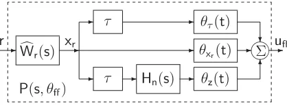
Fig. 2. Structure of the auxiliary adaptive dynamic feedforward systemP (s,ff).

input. In addition to the usual memoryless feedfor-ward term_r(t)r(t)with the adjusted gain_r(t) con-tained inuf(t), see (18),uff(t)includes terms with the

adjusted matrix gains _xr(t), (t) and_z(t). uff(t)

is hence formed by a special adaptively adjusted dy-namic system as a function of the reference signal. By denotingW_r(s)as the input-to-state transfer function (Is−Ar)−1_{Br of the reference model (4), the}

com-putation ofuff(t)can be represented by the block

di-agram inFig. 2.

This dynamic feedforward system constitutes the main contribution of our approach. Note that when the system does not contain delay, the controller struc-ture reduces to the one used in standard multivariable model reference adaptive control[8].

In the next two sections we will design adaptive laws for the two distinct assumptions, given in Sec-tion 2, about the high-frequency gain matrix K_p. First we use the symmetry conditions ofK_p[8] (As-sumption A7.1), and then the as(As-sumption on the signs of the leading principal minors of K_p [2] (Assum-ption A7.2).

5. Adaptive controller: Assumption (A7.1)

Introducing the parameter errors˜f(t)and˜ff(t)and using the adaptive control (17)–(19), the basic tracking error equation (15) can be expressed as

e(t)=Wr(s)Kp[˜Tf(t)f(t)+ ˜ T

ff(t)ff(t)

−∗T

ex(t−)−z∗Tze(t)], (20) where˜f(t)=f(t)−∗f,˜ff(t)=ff(t)−∗ff,∗f =

[∗_e,∗T 1 ,∗

T

2 ,∗r]Tand∗ff= [∗ T

xr,∗ T ,∗zT]T. To design the mechanism of updating the controller matrices, the usual way of MRAC for the delay-free

systems is used, see, e.g. [2]. The augmented vector

ˆ

x(t)= [x, x1, x2]T is introduced, and the state of the corresponding nonminimal realizationC(sIˆ − ˆA)−1Bˆ of W_r is denoted by xˆ_r(t). Then we can write the following state space representation for (20):

de(t)ˆ

dt = ˆAe(t)ˆ + ˆBKp[˜

T

f(t)f(t)+ ˜ T

ff(t)ff(t)

−∗T

lˆTe(tˆ −)−∗zTCeze(t)ˆ ], dzˆ_e(t)

dt =Aezˆe(t)+Belˆ

T_{e(tˆ −),}

ze(t)=Cezˆe(t),

e(t)=y(t)−yr(t)= ˆCe(t)ˆ , ˆ

l= [In×n,0_n×m(−1),0n×m(−1)]T, (21)

wheree(t)ˆ = ˆx(t)− ˆx_r(t), the triple(A_e, B_e, C_e)is a minimal state space realization for the stable transfer matrixH_n(s)from (14), and 0_n×m(−1)is a zeron×

m(−1)matrix.

BecauseC(sIˆ − ˆA)−1Bˆ=W_r(s)is SPR, the triple (A,ˆ B,ˆ C)ˆ satisfies the following equations given by the matrix version of KY Lemma, see, e.g.[14,2],

ˆ

AT_Pˆ_{+ ˆPA}ˆ_{+ ˆQ=0, P}ˆ_Bˆ_{= ˆC}T_{, (22)}

wherePˆ= ˆPT>0 andQˆ= ˆQT>0. SinceAe in (21) is stable, it also holds that

AT

ePz+PzAe+Qz=0, (23)

where P_z=P_zT>0 and Q_z=QT_z>0. We are now ready to state the main result of this section.

Theorem 1. Consider system (1) and the reference model (4). Suppose that assumptions (A1) to (A7.1) hold. Then the adaptive control (17)–(19) with update laws

˙

Tf(t)= −Spe(t)Tf(t),

˙

T

ff(t)= −Spe(t)Tff(t) (24)

guarantee that all the closed-loop signals are bounded and the tracking error e(t)=y(t)−yr(t)converges to zero asymptotically, i.e. lim_t→∞e(t) =0.

quadratic Lyapunov function, an appropriate Lyapunov-Krasovskii functional is added as in[12],

V = ˆeT_Pˆ_{eˆ+ ˆz}T

ePzzeˆ + _t

t−eˆ

T_{(s)Qee(s)ˆ ds}

+tr(˜f− ˆK1)p(˜f− ˆK1)T+tr(˜ffp˜ T ff),

(25)

whereQ_e=QT_e>0,_p=KT_pS_p−1, wherein the known matrixS_p satisfies Assumption A7.1,

ˆ K1= −

r 2[K

−1

p 0 0 0]T (26)

and r is an as yet unspecified positive constant. With this definition of Kˆ1, using p from (25),

e= ˆBT_Pˆ_{eˆfrom (21) and (22),} ˙

f from (24) and

As-sumption (A7.1) we have

tr[ ˆK1p˙˜ T

f] = −tr[ ˆK1pSpe(t)Tf]

= −tr[eT_fKˆ1pSp]

= −r 2e(t)ˆ

T_Pˆ_Bˆ_BˆT_Pˆ_{e(t)ˆ .}

Then some simple computations using (22), (24) and (26) withQˆ=Q+Q_e, Q=QT>0 lead to the deriva-tive of V along the solution of (21),

˙

V|(21)= − ˆeT(t)Qe(t)ˆ −re(t)ˆ TPˆBˆBˆTPˆe(t)ˆ

− ˆzT

e(t)Qzze(t)ˆ − ˆeT(t−)Qee(tˆ −) −2eˆT(t)PˆBˆK_p∗TlˆTe(tˆ −)

−2eˆT(t)PˆBˆK_p∗_zTC_ezˆ_e(t)

+2zˆT_e(t)PzBelˆTe(tˆ −). (27) For convenience, let us define the matricesQe=(qe1+

qe2+qe3)I,Qz=(qz1+qz2+qz3)I, and the scalar

r=r1+r2, whereqei, qziandri (i=1, . . .)are

posi-tive constants. Note that these constants are only used in the process of the proof and not used in the con-trol design, and hence we can suppose that they take arbitrary positive values.

Combining the second and fifth, second and sixth and third and seventh terms of (27), completing the squares and dropping negative terms, and using the known inequality 2T 1T+ T for any

, ∈Rn_{and scalar>0, we obtain} ˙

V|(21)− ˆeT(t)Qe(t)ˆ −qz3zˆT_e(t)zˆe(t)

−qe3eˆT(t−)e(tˆ −)

− ˆeT_(t−)

qe1I −

1 r1

1

ˆ e(t−)

− ˆeT_(t−)

qe2I−

1 qz12

ˆ e(t−)

− ˆzT

e(t)

qz2−

1 r2z

ˆ

ze(t), (28)

where

1= ˆl∗KT_pKp∗TlˆT, 2= ˆlB_eTPzPzBelˆT,

z=CTe∗zKpTKp∗zTCe. (29)

Let us select the values ofr1, r2andqe2such that the

following inequalities are satisfied:

r1>

1

qe1max[1], qe2>

1

qz1max[2]

,

r2>

1 qz2

max[z], (30)

where max() is the maximum eigenvalue of .

Then, we obtain from (28)

˙

V|(21)− ˆeT(t)Qe(t)ˆ −qz3zˆT_e(t)zˆe(t)

−qe3eˆT(t−)e(tˆ −)0. (31)

This implies[5]that V and, therefore,e(t), e(t)ˆ ,zˆ_e(t),

f, f, ff,ff ∈ L∞. This fact is central to the remainder of the stability analysis, which follows di-rectly using the steps in[8].

Because e(t)ˆ = ˆx(t)− ˆx_r(t) and xˆ_r(t) ∈ L_∞, it holds thatx(t)ˆ = [xT(t),x₁T(t), x₂T(t)]T∈L_∞, which implies that x(t), x1(t), x2(t)andy(t) ∈ L∞. Since r(t) is uniformly bounded and the transfer matrix Hn(s) from (14) is stable, f = [eT, x₁T, x₂T, rT]T andff(t)= [x_rT(t), x_rT(t−), zT_r(t)]T are bounded. Consequently u(t)=uf(t)+uff(t) is also bounded. Therefore, all the signals in the closed-loop system are bounded. From (25) and (31) we establish that

ˆ

e(t) and therefore e(t) ∈ L2. Furthermore, using

ˆ

6. Adaptive controller: Assumption (A7.2)

To avoid the quite restrictive Assumption (A7.1), we will use in this section the recent results for multivari-able MRAC design in[2] for plants without delays. The design in[2]is based on theSDU factorization [13]of the high-frequency gain matrixK_p, with the assumption that the signs of the leading principal mi-nors of K_p are known. Such an assumption is less restrictive than the symmetry condition in Assumption (A7.1). The following preliminary lemmas are needed.

Lemma 1 (Costa et al.[2]). Everym×mmatrixK_p with nonzero leading principal minors 1, . . . ,m

can be factored asK_p =SDU, where S is sym-metric positive definite,Dis diagonal, and U is unity upper triangular.

This factorization ofK_p is convenient because of the distinct role played by each of its factorsS, D and U. The role ofSis to assure one that theW_r(s)S is SPR. The rôle ofDis to enable a straightforward extension of the SISOassumption about the sign of the high-frequency gain. The rôle of U is to allow its absorption by the controller parametrization[2].

Lemma 2 (Costa et al.[2]). For anyW_r(s)from (4) a positive definiteS=ST>0 exists such thatW_r(s)S is SPR.

Substituting theSDU factorization ofK_p in the basic error equation (15), and using the decomposition

Uu=u−(Im×m−U)

as in[2], we obtain

e(t)=Wr(s)SD[u(t)−(I−U)u(t)−U∗_ee(t) −U∗T

1 x1(t)−U2∗Tx2(t)−U∗_rr(t)

−U∗T

xr xr(t)−U∗ T

xr(t−) −U∗T

z zr(t)] −Wr(s)SD × [U∗T

ex(t−)+U∗zTze(t)]. (32)

By definingˆ∗_e=U∗_e,ˆ∗₁T=U₁∗T,ˆ∗₂T=U₂∗T,ˆ∗_r= U∗_r,ˆ∗_u=(I_m×m−U)u,ˆ∗_xT

r =U∗ T

xr,ˆ

∗T

=U∗T,

ˆ

∗_zT=U∗T

z , andˆ∗

T

z =U∗zT, we obtain from (32) e(t)=Wr(s)SD[u(t)− ˆ∗ee(t)− ˆ∗

T 1 x1(t)

− ˆ∗2Tx2(t)− ˆ

∗

rr(t)− ˆ∗uu− ˆ∗

T

xrxr(t)

− ˆ∗Txr(t−)− ˆ∗

T

z zr(t)] −Wr(s)SD × [ˆ∗Tex(t−)+ ˆ∗

T

z ze(t)]. (33)

We can rewrite (33) as

e(t)=Wr(s)SD[u(t)−Kf∗T(t)¯f(t)−∗ffT(t)ff(t)]

−Wr(s)SD[ˆ∗Tex(t−)+ ˆ∗zTze(t)], (34) where

Kf∗= [ˆ

∗

e,ˆ∗

T 1 ,ˆ

∗T 2 ,ˆ

∗

r,ˆ∗u]T,

∗

ff= [ˆ

∗T

xr,ˆ

∗T ,ˆ∗

T

z ]T, ¯

f= [eT, x1T, x2T, rT, uT]T,

ff = [x_rT(t), x_rT(t−), zT_r(t)]T. (35)

In order to remove the zero entries from the above parametrization, we introduce, as in [2], the new pa-rameter vectorsfi via the identity

[∗1T

f 1f· · ·∗fkTkf· · ·f∗mTmf]T=Kf∗T¯f. (36)

In addition to the concatenated kth rows of the matrices ˆ

∗_e, ˆ∗₁, ˆ₂∗, ˆ∗_r, each row vector ∗_fkT includes the unknown entries of the kth rows of ˆ∗_u. The strictly upper triangularity ofˆ∗_uensures that the control signal is implementable without singularity.

The corresponding regressor vectors are

1

f(t)= [ ˆ T

f, u2, u3. . . , um−1, um]T,

2

f(t)= [ ˆ T

f, u3, . . . , um−1, um]T,

... mf (t)= [ ˆ

T f]

T_{. (37)}

This new parametrization motives the following con-troller structure instead of (17)–(19)

u(t)= [1T

f (t)1f(t)· · ·kfT(t)kf(t)· · ·mfT(t)

×m

f (t)]T+ T

and gives the following error equation instead of (34)

e(t)=Wr(s)SD   



1T

f (t)1f(t)

...

mT

f (t)mf(t)

 

−  

1∗T

f (t)1f(t)

...

m∗T

f (t)mf(t)

 

+T

ff(t)ff(t)−∗ffT(t)ff(t)

 

−Wr(s)SD[ˆ∗Tex(t−)+ ˆ∗_zTze(t)]. (39) Remark 3. Is it easy to see from (38), that in this case as well as in (17)–(19), the first control component with output feedback

uf(t)= [1Tf (t)1f(t)· · ·kfT(t)

×k

f(t)· · ·mfT(t)mf (t)]T (40)

is identical to the controller for MIMOplants without delay in[2]. In this case, the new additional feedfor-ward component uff(t)has the same structure as in (19).

Introducing the parameter errorsk_f(t)=k_f(t)−

∗k

f , k=1, . . . , mandff(t)=ff(t)−∗ff, the equa-tion for the tracking error follows from (39),

e(t)=Wr(s)SD[(1T

f (t)1f(t)· · ·

kT f (t)

×kf(t)· · ·

mT

f (t)mf(t))T+ T

ff(t)ff(t)]

−Wr(s)SD[ˆ∗Tex(t−)+ ˆ∗zTze(t)]. (41) As in Section 5, the augmented vector x(t)¯ = [x, x1, x2]T is introduced, and the state of the

corre-sponding nonminimal realization C(sI¯ − ¯A)−1B¯ of Wr(s)S, (C¯B¯=S) is denoted byx¯_r(t). Then we can write the following state space representation of (41)

˙¯

e(t)= ¯Ae¯+ ¯BD[(1Tf (t)1f(t)· · ·

kT f (t)

×k

f(t)· · ·

mT

f (t)mf (t)) T₊T

ff(t)ff(t)]

− ¯BD[ˆ∗TlˆT_{e(t¯ −)+ ˆ}∗T

z Cez¯e(t)], ˙¯

ze(t)=Aeze(t)¯ +BelˆT_{e(t¯ −),}

ze(t)=Ceze(t)¯ ,

e(t)=y(t)−yr(t)= ¯Ce(t)¯ . (42)

Because C(sI¯ − ¯A)−1B¯ =W_r(s)S is SPR [2], the triple (A,¯ B,¯ C)¯ satisfies the following equations, as in (22),

¯

AT_P¯_{+ ¯PA}¯_{+ ˆQ=0, P}¯_B¯_{= ¯C}T_{, (43)}

whereP¯ = ¯PT>0 and Qˆ =Q_e+Q. To design the update laws, we use the functional

V = ¯eT_P¯_{e¯+ ¯z}T

ePzz¯e+ _t

t−e¯ T_(s)Q

ee(s)¯ ds

+tr(˜ff−1D¯˜ T ff)

+ m

k=1

(k

f)−

1_|dk_|(k f − ¯K1k)

T₍k

f − ¯K1k), (44)

wherek_f>0,=T>0,D¯=diag{d1. . .dk. . .|dm|}, whereindkare the entries ofD, and

¯

K1k= −r(dk)−1[I, 0, . . . , 0]T. (45)

The vectorsK¯₁k have the same dimension ask_f, and r is an “artificial” gain parameter whose value will be specified later. Let the adaptation algorithm be

˙

kf = −kfsign(dk)kfek, k=1, . . . , m,

˙

Tff= −Sign(D)e(t)Tff(t), (46)

where Sign(D)=diag{sign(d1), . . . ,sign(dm)}. With this adaptation algorithm, the time derivative of (44) along the trajectories of the error system (42) becomes

˙

V|(42)= − ¯eT(t)Qe(t)¯ − ¯re(t)¯ TP¯B¯B¯TP¯e(t)¯

− ¯zT

e(t)Qzz¯e(t)− ¯eT(t−)Qee(t¯ −) −2e¯T(t)P¯BD¯ ˆ∗TlˆTe(t¯ −)

−2e¯T(t)P¯BD¯ ˆ∗_zTCeze(t)¯

Using the same arguments as in Section 5 above, we have

˙

V|(42)− ¯eT(t)Qe(t)¯ −qz3z¯T_e(t)ze(t)¯

−qe3e¯T(t−)e(t¯ −)

− ¯eT_(t−)

qe1I−

1 r1 ¯ 1 ¯ e(t−)

− ¯eT_(t−)

qe2I−

1 qz1

¯

2

¯ e(t−)

− ¯zT

e(t)

qz2−

1 r2 ¯ z ¯

ze(t), (48)

where

¯

1= ˆlˆ

∗

DDˆ∗ T

lˆT, ¯2= ˆlB_eTPzPzBelˆT,

¯

z=CeTˆ∗zDDˆ∗

T

z Ce (49)

and, as in (30), after the choice ofr1, r2andqe2

sat-isfying the inequalities

r1>

1 qe1

max

_¯

1

, qe2>

1 qz1

max

_¯

2

,

r2>

1 qz2max

_¯

z, (50)

we obtain from (48)

˙

V|(42)− ˆeT(t)Qe(t)ˆ −qz2zˆ_eT(t)zˆe(t)

−qe3eˆT(t−)e(tˆ −)0. (51)

By applying the same arguments as in Theorem 1 it can be shown that lim_t→∞e(t) =0.

All this leads to the main result of this section.

Theorem 2. Consider the closed-loop system defined by the plant in (1), the controller in (38), and the updating algorithms in (46) with Assumption 7.2. Then the following two properties hold:

(i) all signals of the closed-loop system are bounded, (ii) lim_t→∞e(t) =0.

7. Example

To illustrate the application of the proposed adaptive scheme, let us consider an unstable system described

by the model

˙ x(t)=

1.0 0

0 1.0

x(t)+

2.0 3.0 4.0 5.0

x(t−)

+

−1.0 2.0 3.0 1.0

u(t),

y(t)=

1.0 0 0 1.0

x(t), x(0)=

1.0 −1.0

. (52)

To build the adaptive controller we chose the reference model

˙ xr(t)=

−1.0 0 0 −1.0

xr(t)+

1.0 0

0 1.0

r(t),

yr(t)=

1.0 0 0 1.0

xr(t), x(0)=

0 0

. (53)

In this task all the parameters exceptare unknown to the controller. The only information available to the controller is the structural information given in As-sumptions A1–A7. The parameters of the non-delayed part of the plant model (52) are taken from[6].

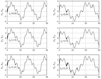
Simulation results are shown inFigs. 3–5, where we show the time responses of the output of the planty(t), the output of the reference modely_m(t), the tracking errore(t)and the tracking error norm.

Figs. 3 and 4 were generated by the plant model (52), the controller (38), (46), and the reference model (53) with

r(t)=

sin(t)+2 sin(3t)+3 sin(0.5)t cos(0.5t)+2 cos(2t)+3 cos(0.3t)

and the plant state delay=5. The parameter values of the controller are sign(d1)= −1, sign(d2)=1 and

1

f =2f=100.

The robustness of the adaptive control law to delay uncertainty is illustrated inFig. 4, where we show the time history of the plant and reference model outputs yt=[y1(t), y2(t)]Tandyr(t)=[yr1(t), yr2(t)]T, for the case, when the delay valuec, used in the controller, differs from the plant delay value.

Fig. 5 was generated with the use of controller (17)–(19), (24), the plant model (52) with=3, and the reference model (53) with a square-wave reference signalr(t). We chose the parameter

Sp=

−14.2857 28.5714 300.00 14.2857

0 5 10 15 20 25 30 -4

-2

-4 -2 0 2 4

y1

, y

r1

0 5 10 15 20 25 30

0 2 4

y2

, y

r2

0 5 10 15 20 25 30

0 0.5 1

error norm

Time

τc=τ=5

τc=τ=5

τc=τ=5

Fig. 3. Simulation of the adaptive control system for the plant with state delay (52) and the controller (38), (46). The upper, middle and lower graphs show the time history of the plant and reference model outputsyt= [y1(t), y2(t)]T,yr(t)= [yr1(t), yr2(t)]T, and the error norm, respectively.

0 10 20 30

-4 -2 0 2 4

0 10 20 30

-4 -2 0 2 4

0 10 20 30

-4 -2 0 2 4

0 10 20 30

-4 -2 0 2 4

0 10 20 30

-4 -2 0 2 4

0 10 20 30

-4 -2 0 2 4

y1

, y

r1

y1

, y

r1

y1

, y

r1

y2

, y

r2

y2

, y

r2

y2

, y

r2

τc=0.8τ

τc=τ=5

τc=1.2τ τ

c=1.2τ τc=τ=5 τc=0.8τ

0 5 10 15 20 25 30 0

0.5

-0.5

-0.5

-0.5 e1

e2

0 5 10 15 20 25 30

0 0.5

0 5 10 15 20 25 30

0 0.5 1

-1

Time r1

, r2

r₁

r₂

Fig. 5. Simulation of the adaptive control system for the plant with state delay (52) and the controller (17)–(19), (24). The upper, middle and lower graphs show the time history of the error componentse1(t),e2(t)and the reference model inputsr1(t)andr2(t), respectively.

The demonstrated robustness property allows us to hope that in the future it will become possible to re-lax the restrictive assumption about knowing the plant delay. This topic is currently under investigation.

8. Conclusion

Two new output feedback adaptive control schemes based on Model Reference Adaptive Control (MRAC) and adaptive laws for updating the controller pa-rameters are developed for a class of linear multi-input–multi-output (MIMO) systems with state delay. An effective controller structure established on a new error equation parametrization is proposed to achieve tracking with asymptotical zero error. To achieve exact asymptotical tracking, we introduce, in the stan-dard MRAC structure for the plants without delay, a new adaptive feedforward control component as an output of a dynamical system driven by the reference signal. The feedforward prefilter design procedure is developed to determine the necessary feedforward dynamic system which satisfies design conditions for two different assumptions about the prior knowledge

of the high-frequency matrixK_p: the symmetry as-sumption of[8], and the assumption on the signs of the leading principal minors ofK_p [2], respectively. The proposed adaptive control law constructions make economical use of known results of MIMOmodel ref-erence adaptive control to the considered class of de-layed system. Adaptive laws are developed using the SPR-Lyapunov design approach. A simple simulation example is given to show the potential of the proposed technique. This work is the first asymptotic exact zero tracking results for this class of systems in the frame-work of the certainty equivalence approach.

Acknowledgements

References

[1]F. Blanchini, E.P. Ryan, A Razumikhin-type lemma for functional differential equations with application to adaptive control, Automatica 35 (1999) 809–818.

[2]R.R. Costa, L. Hsu, A.K. Imai, P. Kokotovi´c, Lyapunov-based adaptive control of MIMOsystems, Automatica 39 (7) (2003) 1251–1257.

[3]S.G. Foda, M.S. Mahmoud, Adaptive stabilization of delay differential systems with unknown uncertain bounds, Int. J. Control 71 (2) (1998) 259–275.

[4]K. Gu, S.-I. Niculescu, Survey on recent results in the stability and control of time-delay systems, J. Dyn. Syst. Meas. Control 125 (2) (2003) 158–165 (special issue: Time delayed systems).

[5]J.K. Hale, S.M.V. Lunel, Introduction to Functional Differential Equations, Springer, New York, 1993.

[6]L. Hsu, R. Costa, A.K. Imai, Multivariable adaptive control with transient overparametrization, in: Proceedings of the 42nd IEEE Conference on Decision and Controls, Hyatt Regency Maui, Hawaii, USA, 2003.

[7]A. Ilchman, E.P. Ryan, On gain adaptation in adaptive control, IEEE Trans. Automat. Control 48 (5) (2003) 895–899. [8]P.A. Ioannou, J. Sun, Robust Adaptive Control, Prentice-Hall,

Englewood Cliffs, NJ, 1996.

[9]M.S. Mahmoud, Adaptive control of a class of time-delay systems with uncertain parameters, Int. J. Control 63 (5) (1996) 937–950.

[10]B.M. Mirkin, Combined direct and indirect adaptive control for plants with state time delay, Vestnik MUK 13 (1) (2001) 45–48 (in Russian).

[11]B.M. Mirkin, P.O. Gutman, Output adaptive model reference control of linear continuous state-delay plant, in: Proceedings of 15th International Symposium on the Mathematical Theory of Networks and Systems, 12–16 August, Notre Dame, USA, 2002.

[12]B.M. Mirkin, P.O. Gutman, Output-feedback model reference adaptive control for continuous state delay systems, J. Dyn. Syst. Meas. Control 125 (2) (2003) 257–261 (special issue: Time delayed systems).

[13]A.S. Morse, A gain matrix decomposition and some of its applications, Syst. Control Lett. 21 (1993) 1–10.

[14]K.S. Narendra, A.M. Annaswamy, Stable Adaptive Systems, Prentice-Hall, New York, 1989.

[15]S. Oucheriah, Adaptive robust control of class of dynamic delay systems with unknown uncertainty bounds, Int. J. Adapt. Control Signal Process. 15 (2001) 53–63.

[16]E.P. Ryan, C.J. Sangwin, Controlled functional differential equations and adaptive stabilization, Int. J. Control 74 (1) (2001) 77–90.

[17]E.P. Ryan, C.J. Sangwin, Controlled functional differential equations and adaptive tracking, Syst. Control Lett. 47 (2002) 365–374.

[18]S. Sastry, M. Bodson, Adaptive Control Stability, Convergence, and Robustness, Prentice-Hall, Englewood Cliffs, NJ, 1989.