CHAPTER 3 -PHYSICAL PROPERTIES OF SEAWATER
Historically ocean temperature and salinity profiles were measured by arrays of Nansen
bottles, with reversing thermometers. A typical deep ocean cast would consist of the
deployment of 20 to 30 bottles on a steel winch cable; from which temperatures with
typical precisions of ± 0.01 oC and salinities with precisions of ± 0.01psu could be
obtained. The difference between protected and unprotected reversing thermometers
was used to infer pressure (and hence depth) to within ± 2m. Historically, chemical
titration methods, assuming constant proportions among the different ions in seawater,
were used to determine salinity according to the relation
) / ( Cl 1.805 + 0.03 = ) S( oo o psu ,
where Cl (parts per thousand) is the “chlorinity” of a water sample.
The modern oceanographic instrument used to measure continuous distributions of
conductivity, temperature versus depth; (actually pressure) is called a CTD. The variety
of electronic CTD instruments commercially-available today have enough resolution to
resolve differences of 0.01 oC to 0.001oC in temperature ; equivalent 0.01 psu to 0.001
psu in salinity; and 0.10m to 1.00m in pressure on centimeter to meter-vertical scales.
Salinity is determined from precision measurements of seawater conductivity C and
temperature T and well-known, complicated relationships that can be approximated for
our purposes by:
C) T( 0.73 -) cm mmho ( C 1.02 + 3.55 = )
S(psu ° .
Such measurements were used to infer the generic temperature, salinity and density
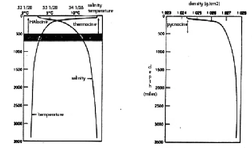
profiles in Figure 3.1. The upper ocean warmth, freshness and “lightness” relative to the
deeper ocean are major features of these profiles. Later we will explore the real
Figure 3.1 Generic subtropical temperature, salinity, and density profiles exhibit regions of large change; thermocline, halocline, and pycnocline, respectively. (Duxbury and Duxbury, 1984)
Seawater Density
Probably the most important dynamic property of seawater is its densityρ . In general
the observed differences in seawater density are due to the combined effects of
variability in temperature T, salinity S, and pressure P. Though relatively small (the
range of sea surface densities is from 1.024 to 1.030 gm/cm3) horizontal differences in
density produce horizontal pressure forces which in turn produce ocean currents.
Symbolically the following relation
expresses the dependence of the seawater density (mass per unit volume) of a water
parcel (Figure 3.2) on its measured or insitu salinity, S, insitu temperature, T, and
insitu pressure, p, where insitu refers to values of these variables at the location of the )
(or P) T, (S,
=ρ ρSTP
water parcel of interest.
Changes in the value of insitu density can be explored by considering its total
differential, dρ , as follows
. | d d |
dT d |
d d
d , , , dP
P dT dS
STS SP ST
ρ ρ
ρ
ρ= + +
Variability in density can be explored more conveniently in terms of insitu density
anomaly, σSTP, which is defined as
Thus surface density anomalies vary from 24.0 to 30.0 mg/cm3.
Compressibility (or pressure) effects
The most important (or first order) effect of hydrostatic pressure on density is to
decrease the volume of a water parcel by squeezing the same molecules closer together;
Figure 3.2 A parcel of seawater that is small enough so that the measured or insitu temperature T, salinity S, and pressure P is homogeneous for practical purposes .
. 10 x 1) -(
= 3
STP
STP ρ
thus there is an increase inρSTP.
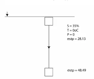
For example, if we consider what happens to a water parcel at the sea surface (with the
given properties) after we move adiabatically (without heat loss or gain) to a depth of
4000 m where the pressure is ~400 atmospheres or 6000 psi (Figure 3.3).
In this example the pressure effect on σSTPis nearly 100%. In general this very large
pressure effect obscures density changes due to the natural variability of temperature
and salinity. Therefore oceanographers find it convenient to compare the density of
water parcels in terms of the quantity called sigma-t and defined
where P is gauge pressure which is zero at the sea surface.
This definition in effect removes the very large pressure effect on σSTP by evaluating
σSTPat the insitu values of S and T and the sea surface pressure. σT is a complicated
function of S and T and can be found in Table 11-1, Knauss.
A secondary (or second order) effect of an increase in hydrostatic pressure is the
increase of measured temperature, Tinsitu, at the approximate rate of 0.1NC per
kilometer of depth increase. The adiabatic compression of a water parcel causes
increased molecular activity and thus an increased observed temperature.
For example, surface values of Ssurf = 35% and Tsurf = 5.00NC an adiabatic compression
to a depth of 4000 m will produce a Tinsitu = 5.45NC. Conversely an adiabatic
expansion from a depth of 4000 m with Tinsitu = 5.00NC will lead to Tsurf = 4.56NC.
This non-linear adiabatic heating and cooling is reasonably well-understood and is
summarized in Table 11-6, Knauss.
These tables can be used to compute a quantity called potential temperature, θ . , or
Tsurf. Potential temperature is Tinsitu which has been corrected for compressibility
effects.
Figure 3.3. The dependence of seawater density anomaly on pressure.
When θ is used rather than Tinsitu to compute density anomaly the quantity potential
density anomaly, or sigma-θ or σθ is appropriate and is defined
Thus we have defined a density-related term, σθ, whose value depends on the intrinsic
properties of a water parcel, θ and S, (determined by air-sea interaction processes at
the sea surface) only. The external influence of pressure on volume and temperature of
the water parcel have been eliminated. The use of σT and σθ is convenient when
assessing the stability of a water column.
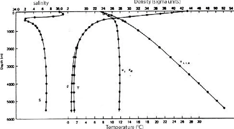
This comparison of T and θ and σT and σθ for data from the North Pacific in
Figure 3.4 shows the important the pressure effects on temperature, especially for .
=σS, ,P 0
depths greater than 4 km. Note the misleading stability implied by the σT profile.
For computing of ocean currents from water properties, it is convenient to use the
inverse of density or specific volume according to
A related quantity, known as the specific volume anomaly, δ , is defined
where α35,0,P is the specific volume of a “standard ocean” that is defined so δ is
normally a positive value. δ is somewhat analogous to σ .
Figure 3.4 Comparison of insitu temperature and potential temperature profiles (left); sigma-t and sigma-? profiles.(Knauss, 1978)
. 1 =
STP STP
ρ α
,
-=αSTP α35%,0 C,P
For computational purposes δ can be expressed as follows
where these components can be obtained from the indicated tables in Knauss. The
oceanic range of δ is 50 - 100 x 10-5 or 50-100 cl/ton, where δ units are
kg 10 ml 10 = d/ton or /gm cm = ] [ 3 3 δ .
WATER COLUMN STABILITY
Normally density increases with depth because of the natural tendency for more dense
water parcels to sink quickly to their equilibrium depths water parcels which are
displaced vertically from this stable configuration will oscillate and eventually return to
their equilibrium depth. The strength of the stability is related to the vertical potential
density gradient
where
A measure of the strength of stability is the natural frequency at which a water parcel
would oscillate vertically in the ocean. This is called the buoyancy or Brunt-Väisälä
frequency, which varies with depth according to
Thus, it is the slope of the vertical distribution of potential density anomaly, σθ, which
can be used to assess the stability of the water column or its resistance to vertical
motion. For shallow depths, where temperatures and salt effects dominate pressure
effect, profiles of σT are adequate for assessing water column stability.
TEMPERATURE AND SALINITY DIAGRAMS
A useful tool in assessing the stability of a particular water column is a T (orθ ) - S
diagram; on which T (or θ ) and S measurement pairs are plotted. Because σT (or
σθ) is a unique function of T(θ ) and S, isopleths of σT (or σθ)can be inscribed on
the T(θ ) - S diagram as (Figure 3.5).
Figure 3.5. The density of seawater, abbreviated as ρ, varies with temperature and salinity. The pressure effect is not included here.(Duxbury & Duxbury, 1984)
10 x z E
or sec rad = [N] ; z g -= (z)
N pot -3
o 2
∂ ∂ − ≅ ′
∂ ∂
ρσ ρ
ρ
One of the important consequences of the nonlinearity of the σT (σθ) isopleths is that
. C 6 near |
dT d > | dT d C 28
near ° σT35% σT35% °
This nonlinear feature of density plays an important role in polar water formation to be
discussed later. (The sensitivity of σT to salinity changes does not vary much from high
to low temperatures.) With our crude understanding of the important air/sea interaction
processes and some exposure to the terminology used by oceanographers we can begin
to explore the distributions of density, temperature and salinity.
Surface Distribution of Density
Because the surface ocean temperatures and salinities are most directly influenced by
air/sea interaction processes, it is not surprising that the north-south horizontal gradients
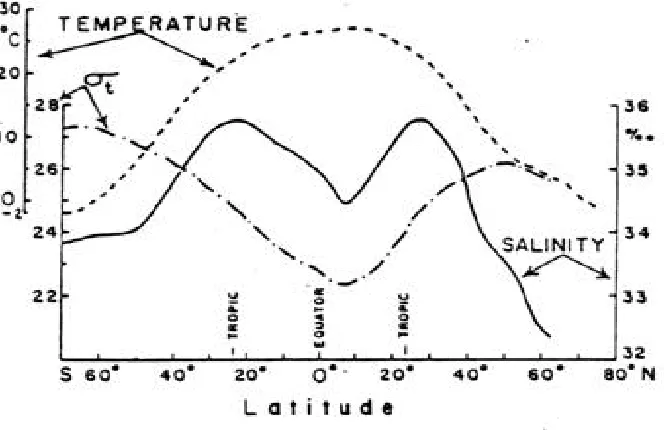
of density (and temperature) are the largest. Thus the latitude variation of σT (Figure
3.6) shows that density (σT) is primarily determined by temperature variation - except
in the polar regions where dσT/dT is relatively less and salinity variations are significant.
Also note that the minimum in sT is located at a latitude to about 5NN (corresponding
to the maximum in T - the “meteorological equator”).
Horizontal and Vertical Distributions of Temperature
The zonal distributions of surface temperature (and density) in summer (Figures 3.7)
and winter (Figure 3.8) are consistent with the strongly zonal distribution of atmospheric
circulation..
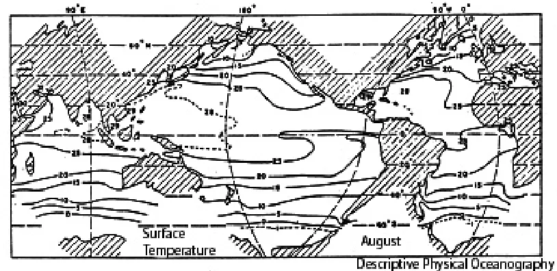
Figure 3.7 Surface temperature of the oceans in August. (Pickard & Emery, 1982)
Figure 3.8 Surface temperature of the oceans in February. (Pickard & Emery, 1982)
One of the principal features of the oceans is its vertical stratification of properties. For
gradients discussed above. At the equator Tsurf = 25oC and T1000m = 5oC, thus vertical
temperature gradient at the equator is
km C 20 = | dz dT
equ
°
(Figure 3.9). On the other hand
one must move 5000 km northward on the surface before Tsurf = 5 oC. Thus the
northward temperature gradient at the ocean surface
is .
km C 10 x 4 = km
C 5000
20 = | dy
dT -3
surf
° °
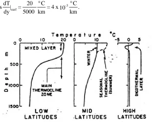
Figure 3.9. Typical mean temperature profiles in the open ocean. (Pickard & Emery, 1982)
Seasonal Temperature Distributions
The seasonal variability of vertical temperature stratification is summarized in Figure
3.10. The four general zones that define these profiles are described next.
(1) The mixed layer is found between the surface and 20-60 m depths and strongly
Figure 3.10. The seasonal variability of a typical subtropical temperature profile. (Duxbury & Duxbury, 1984)
(2) The seasonal thermocline is usually found in the upper 100 m and is a feature which
will change seasonally in intensity. Typical vertical gradients:
C/km) (60
C/m 0.06 = dz
dt ° °
change with seasons.
(3) The main or permanent thermocline is found between 800-1500 m and is maintained
by the general circulation. Typically
km C 22 or m
C 0.222 = dz
dT ° °
for this region.
(4) The deep water is nearly isothermal and has typical .
km C 0.8 or m
C 0.0008 =
dz
dT ° °
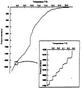
It is important to realize that the “smoothly-varying” profiles of temperature profile, like
the one to the left in Figure 3.11, is really highly structured as depicted to the right in
Figure 3.11. The rather large “steps” in the temperature trace in aredue to small scale
mixing processes discussed later.
Figure 3.11. Sharp stepwise temperature gradient can be easily seen on the blown -up sectio n of the temperatures traced from the Mediterranean Outflow Region (34oN, 11oW). The temperature steps are generally less than 0.1oC and occur at about 10-m intervals. (After Magnell, B., 1976a “Salt Fingers in the Mediterranean Outflow Region (34oN, 11oW) using a Towed Sensor”, J. Phy. Oceanogr., 6.) (Knauss, 1978)
Surface Distribution of Salinity
The ocean surface distributions of salt are less zonal and less variable than ocean
surface temperature because salt variability is controlled by the spatial variability in the
evaporation, precipitation and coastal freshwater outflow. Global scale surface salinity
Figure 3.12 Surface salinity of the oceans in August.
The lowest salinity 0 to 30 psu are found in estuarines and polar environments near
glaciers. Mid-range salinities (30psu-34psu) are typically found in coastal regimes.
Typical oceanic salinities range from 33psu to 37psu with Atlantic salinities being slightly
higher than Pacific salinities due to the Mediterranean outflow. Semi-enclosed regions,
such as the Mediterranean and Red Sea, exhibit salinities of 37psu to 41psu
respectively.
Vertical Profiles of Salinity
Like temperature, oceanic salinities are also vertically stratified because their distribution
is strongly influenced by air/sea interaction processes at the sea surface plus the deep
circulation in the ocean (see Figure 3.13). Unlike temperature it is more difficulty to
generalize about the vertical distribution. Because fresh and salt water sources are not
distributed zonally, like the heat sources, the salt distributions are less easily
summarized.
In general, however,
(a)A salinity maximum occurs at about 100 m depth in the tropics and is due to
(b)A salinity minimum is found between 600 m and 1000 m in the equatorial tropics and
subtropic latitudes and is due to circulation and mixing,
(c)At high latitudes there is a tendency toward low surface salinity.
Low and mid-latitude profiles, which exhibit strong vertical salinity gradients or
haloclines in the upper 800 m, are shown in Figure 3.13. Note that these profiles have
a destabilizing influence on the water column. However, temperature effects
predominant in these regions. When salt destabilizes the water column small scale
processes which lead to the structure seen in Figure 3.13 can result.
Figure 3.13 Typical mean salinity profiles in the open ocean. (Pickard & Emery, 1982)
Vertical Distribution of Density
Because ocean density variation is determined principally by ocean temperature, density
exhibits the same kind of stratification as temperature (see Figure 3.14) - principal
stratification in the upper two kilometers of the ocean. However, as shown by he
vertical section of isotherms in Figure 3.15, the strength of the stratification decreases as one moving poleward from the tropics.
gradient
z g -= N or , z -or , z
- pot pot
∂ ∂ ∂
∂ ∂
∂ ρ
ρ σ
ρ θ
increases (remember z is positive
upwards). The regions of maximum stability within the water column are called
pycnoclines. Because stable vertical stratification resists the vertical motion of water,
there is a strong tendency for water parcels to move along isopycnals or isopleths of
density (σT or σθ). The vertical section of density in Figure 3.15 suggests a polar
origin to the deep water found at mid-latitudes and equatorial regions.
Figure 3.15 Density (σT) in a south-north section of t he western Atlantic (after Wüst). (Pickard & Emery, 1982)
Sound Transmission in the Sea
The atmosphere transmits light (and other electromagnetic radiation) much better than it
transmits sound. While being relatively opaque to electromagnetic radiation
transmission, the ocean is transparent to sound transmission. Thus sound has become
an important tool for studying the ocean. Difficulties arise however because the profiles
of sound speed vary with depth in a number of different ways. As Figure 3.16 shows
the sound transmission paths vary also.
Of particular interest here is understanding how the distribution of the speed of sound,
Cs varies with ocean properties. Like other physical properties of the ocean the speed
of sound depends upon the local values of temperature, salinity and pressure. It can be
expressed symbolically as follows
where T=θ +TA
P), S, (T, C =
with TA being the part of T due to adiabatic compression.
(i.e. dTA/dz ~ - 0.1 oC/km)
Therefore we can write
By taking the differential of this relation and forming a quantity we define as the
fractional change of speed of sound with depth or
where ?A is the fractional change of the speed of sound in an adiabatic ocean and a, ß
are constants.
We also know that
Therefore the fractional change of ρpot with depth is
where a and b are constants.
) T S, , ( C =
Cs s θ A
+ z S + z = z C C 1 A s s γ β θ α ∂ ∂ ∂ ∂ ∂ ∂ S) , ( = or P) S, (T,
=ρ ρpot ρpot θ
ρ , z S b + z a = z 1 pot pot ∂ ∂ ∂ ∂ ∂
∂ρ θ
The differential relations for Cs and ρpot depend on the vertical gradients of θ and S
and can therefore be combined. Without the gory detail the result is a relation between
fractional sound speed change and the square of the Brunt-Viäsälä frequency plus the
compressional effects of pressure,
We can solve for Cs(z) from the relation above (Figure 3.17 and Appendix B).
There are several observations we can make about the shape of this curve; namely
(a) The speed of sound decrease with depth above 1.2 km due to dominant effects
of θ and S.
(b) The speed of sound increases with depth below 1.2 km due to the dominance of
pressure effects (in the absence of θ ,S variability).
The minimum sound speed occurs at a depth near the depth of the main pycnocline. The
consequences of this sound speed distribution are important for the way sound travels in
the ocean. We can explore the important features by considering what happens when
we explode a depth charge at the depth of the minimum sound speed (~1.2 km depth)
Cs1. The acoustic energy radiates spherically (locally) in the region of the charge.
Figure 3.17. Because sound rays are always bent toward the lower velocity, a sound minimum tends to trap
sound waves and to “channel” them. A sound source in the deep sound channel can often be heard hundreds and even thousands of miles away. The sounds that travel those long distances are of low frequency (the
order of 100 to 1,000 c/sec) because low-frequency is less attenuated than high frequency. Although the ocean is reasonably “transparent” to sound waves, it is not completely so, and over a wide range of
frequency, attenuation increases as the square of the frequency; thus a doubling of the frequency increases
the attenuation by four times, which means that long-range sound transmission is best at low frequencies. Frequencies as low at 100 c/sec (with a corresponding wavelength of about 15 m) are commonly used for
very long-range sound transmissions. Fresh water is even more transparent than salt water to the
transmission of sound; for a given frequency the attenuation is 100 times less in fresh water. The difference is caused by a chemical interaction of the sound waves with one component of the sea salt, the magnesium
All energy is refracted along “ray paths” governed by Snell’s Law i.e.
whereθ′is the elevation above horizontal for the particular ray of interest.
(Choose as initial angleθ1′,then Snell’s Law governs the angle of the ray, θ′,as the
energy propagates into regions of Cs(z)).
The only energy to be transmitted horizontally is contained along ray paths between the
surface limited ray (SLR), the bottom limited ray (BLR) and the horizontal. Energy
travels fastest along the SLR/BLR ray and slowest along the horizontal. However all
energy in this “envelope” eventually focuses on the convergence zone at the depth of the
minimum sound speed about 50 km “downstream”. Since there is a tendency for sound
concentration (as different rays crisscross) along the depth of minimum sound speed the
region is referred to as the “sound channel”.
It turns out that in practice the effective depth range of the sound focusing properties of
the ocean is from 1 to 2 km and its existence is used to track SOFAR floats, which are
ballasted to be neutrally buoyant and transmit only a few watts of acoustic energy over
distances of 10,000 km.
A more recent application - acoustic tomography uses differences in sound transmission
times to infer changes in ocean property and current structure. One such experiment
seeks to monitor the long term change in the average temperature of the ocean. Figure
3.18 summarizes a pilot study for such an experiment.
, constant =
cos C = cos
C
1 1 s s
θ
What’s the Sound of One Ocean Warming?
Oceanography has made a noises in the Indian Ocean (“heard” in Bermuda!) that could
be used to measure global warming.
Figure 3.18. Straight shot. Sound waves generated at Heard Island may be detected by hydrophones at Bermuda and San Francisco, as well as other
Chapter 3 - Appendix: Sea Water Density Terminology
Quantity Units Accuracy of Measurement Typical Range
Classical Modern
T
Temperature ( F-32)
9 5 =
C °
° 0.02
oC abs: 0.005oC
diff: 0.001oC
-0.2 to 30oC
S Salinity
gm/kg or o/oo 0.02 o/oo 0.0024 o/oo 33-37 o/oo
Cl Chlorinity
gm/kg
P Pressure
decibars = 105 dynes/cm2 [weight of 1m of sea
water]
abs. 25 db abs. 1.5 db
diff. 0.01 db
0.6000 db ρSTP Density gm/cm3 cm gm
10-5 3
cm gm
10-6 3
cm gm 1.07 to 1.03 3 σSTP Density anomaly = (ρSTP -1) x 103
10-2 10-3 30-70
0
ρST
Density at atmospheric pressure
gm/cm3
cm gm 10-5 -3
cm gm
10-6 3
cm gm 1.028 -1.023 3 σT
Density anomaly at atmospheric pressure-“Sigma-T”
= (?S,T,O-1) x 103
10-2 10-3 23-28
θ
Potential temperature
?C 0.02?C abs: 0.005 oC
diff: 0.001 oC
-0.2-30 oC
ρSθP = 0 gm/cm
3
10-2 10-3 23-28
σθ
Potential density anomaly cm
gm
10-3 3
δSTP
Specific volume
cm3/gm (or ml/gm) 10-5 10-6 0.02-0.97
δ δ δ δ δ
δ = S+ T+ ST+ SP+ STP
Specific volume anomaly
(αSTP−α35,0P)
kg 10 ml 10 = ton cl 3
10-5 10-6 0.02-0.97
δ δ δS TP SP ST= − −
∆
Chapter 3 - Appendix: Other Physical Properties of Sea Water
Quantity Definition Units Typical Values
K Compressibility ∂ ∂ p STP STP 1 - α
α gmcm
cm
-sec2 4 x 10⁻⁵
ß
Coefficient of Thermal Expansion
T 1 STP STP ∂ ∂α α C 1 ° 10-4 µ Molecular Viscosity
constant of proportality between shear stress and velocity gradient
sec cm-gm 0.02 ν Kinematic Viscosity ρ µ/ sec
cm2 0.02
k
Thermal Conductivity
constant of proportionality between heat flux and temperature gradient
sec C- cm-cal ° 10-3 Cp
Specific Heat (at constant pressure)
amount of heat per gm to warm substance 1 oC
C gm cal ° 1 L
Latent Heat of Evaporation
amount of heat to evaporate one gm of substance
gm cal
gm- 600
Surface tension 75.64 - 0.144 + 0.399Cl
cm dyne
2
75
Vs Speed of Sound
K 1 =
STP
ρ sec
cm 1.5 x 10⁵
C Speed of Light
---
sec
cm 2.3 x 10¹⁰
n Refractive Index
Chapter 3 - PROBLEMS
Problem 3.1. Water Properties
a) Sea Water Density
The following table lists the measured values of pressure Pinsitu (decibars or dbars), temperature Tinsitu (°C) and
salinity S ( practical salinity units or psu) at an oceanic hydrographic station.
Produce the Tinsitu-S curve for these data on the form provided below.
Pinsitu
(dbars)
Tinsitu
(°C)
θ (°C)
S
(psu) σT σθ ∆TS δPT δPS δ α35,o,p α ρ
0 24.84 35.031
180 13.01 35.291
740 5.01 34.488
1505 4.15 34.950
5030 1.10 34.754
7020 1.37 34.755
b) Potential Temperature
Assuming that the adiabatic temperature gradient dT/dP in the ocean is a constant 0.14°C per1000 decibars,
estimate the potential temperature θ of the water at the different temperature Tinsitu and pressure Pinsitu. (Hint:
Suppose T(P) = AP + B. What are A and B? Remember that T(P =0) =θ ).
d) Estimate the rest of the information in the table, including the potential density anomaly
1000 1] 0) P , T (S,
[ = = − ×
= ρ θ
σθ , from the oceanographic tables provided. Are the density anomaly values
consistent with those on the T-S and θ -S diagrams?
e) Using your new knowledge of global ocean water properties “guess” the region of the world's oceans where
Problem 3.2. Oceanographic Vertical Sections
a) On page 33, you are provided with an array of measured temperature distributions in an unknown coastal zone.
On page 32 you are provided with a sub-sampled (i.e. under-sampled) version of the page 33 temperatures.
Contour the page 32 and page 33 vertical sections of temperature data using 6.0, 6.5, 7.0, 7.5, 8.0, and 8.5°C
isotherms where appropriate. Make a guess as to what processes may be affecting the observed temperature
distribution.
b) On page 34, find the measured salinity distribution based on several Nansen bottle casts. Contour these results
in terms of 33.20, 33.40, 33.60, 33.80 psu isohalines.
c) On the page 35, compute all possible σT values and then contour the isopycnals starting with σT = 26.0 at ∆σT
= 0.1 increments.
d) Now plot T-S diagrams for the 7 profiles data. What can you say about the static stability of each of the
Temperature (°C) Section - I
6.4 6.6 7.3 7.4 7.5 7.8 7.9 7.8 7.6 7.9 7.8 8.1 8.2
0 • • • • • • • • • • • • •
20 ° ° ° ° ° ° ° ° ° ° ° ° °
40 •7.0 ° •7.7 ° •7.8 ° •8.1 ° •7.9 ° •7.9 ° •8.2
60 ° ° ° ° ° ° ° ° ° ° ° ° •
80 •7.8 ° •7.6 ° •7.7 ° •8.2 ° •7.9 ° •7.8 ° •8.3
100 ° ° ° ° ° ° ° ° ° ° ° •
120 •7.6 ° •7.6 ° •8.0 ° •7.9 ° •8.0 ° •8.4
140 ° ° ° ° ° ° ° ° °
160 ° •7.6 ° •8.0 ° •8.5 ° •8.6
180 °7.6 °7.6 °8.4 °8.6 °8.8 °8.8
Temperature (°C) Section - II
6.4 6.6 7.3 7.4 7.5 7.8 7.9 7.8 7.6 7.9 7.8 8.1 8.2
0 • • • • • • • • • • • • •
20 °6.5 °7.1 °7.6 °7.7 °7.8 °7.9 °8.0 °7.9 °7.9 °8.1 °7.9 °8.1 °8.2
40 •7.0 °7.5 •7.7 °7.8 •7.8 °7.9 •8.1 °7.9 •7.9 °8.1 •7.9 °8.1 •8.2
60 °7.5 °7.6 °7.6 °7.7 °7.8 °7.9 °8.0 °7.9 °7.9 °8.1 °7.9 °8.1 •8.2
80 •7.8 °7.7 •7.6 °7.7 •7.7 °7.9 •8.2 °7.9 •7.9 °8.2 •7.8 °8.1 •8.3
100 °7.7 °7.6 °7.7 °7.7 °7.9 °8.2 °8.0 °7.9 °7.9 °8.0 °8.1 •8.4
120 •7.6 °7.6 •7.6 °7.9 •8.0 °7.9 •7.9 °8.1 •8.0 °8.2 •8.4
140 °7.6 °7.7 °7.8 °7.7 °7.8 °8.1 °8.2 °8.4 °8.5
160 °7.6 •7.6 °7.8 •8.0 °8.1 •8.5 °8.6 •8.6
180 °7.6 °7.6 °8.4 °8.6 °8.8 °8.8
Salinity (psu) Section
33.18 33.19 33.21 33.30 33.41 33.42 33.38 33.39 33.41 33.44 33.46 33.48 33.50
0 • • • • • • • • • • • • •
20 ° ° ° ° ° ° ° ° ° ° ° ° °
40 • ° • ° • ° • ° • ° • ° •
33.20 33.25 33.30 33.35 33.43 33.46 33.48
60 ° ° ° ° ° ° ° ° ° ° ° ° •
80 • ° • ° • ° • ° • ° • ° •
33.27 33.29 33.35 33.42 33.45 33.47 33.50
100 ° ° ° ° ° ° ° ° ° ° ° •
120 • ° • ° • ° • ° • ° •
33.31 33.39 33.43 33.46 33.50 33.52
140 ° ° ° ° ° ° ° ° °
160 ° • ° • ° • ° •
33.50 33.65 33.70 33.80
180 ° ° ° ° ° °
200 •
Density (σT Units) Section
0 • • • • • • • • • • • • •
20 ° ° ° ° ° ° ° ° ° ° ° ° °
40 • ° • ° • ° • ° • ° • ° •
60 ° ° ° ° ° ° ° ° ° ° ° ° •
80 • ° • ° • ° • ° • ° • ° •
100 ° ° ° ° ° ° ° ° ° ° ° •
120 • ° • ° • ° • ° • ° •
140 ° ° ° ° ° ° ° ° °
160 ° • ° • ° • ° •
180 ° ° ° ° ° °
Salinity (psu)
33.0 33.2 33.4 33.6 33.8 34.0
10.0
9.0
8.0
C)
7.0
6.0
Problem 3.3 Water Column Stability
Given what you know about properties that affect the density of seawater:
a) Would coastal regions have a high or low Brunt-Vaisala frequency relative to the central oceanic regions?