International Doctorate School in Information and Communication Technologies
DISI - University of Trento
Discrimination of Computer Generated
versus Natural Human Faces
Duc-Tien Dang-Nguyen
Advisor:
Prof. Giulia Boato
Universit`a degli Studi di Trento
Co-Advisor:
Prof. Francesco G. B. De Natale
Universit`a degli Studi di Trento
-The development of computer graphics technologies has been bringing realism to computer generated multimedia data, e.g., scenes, human char-acters and other objects, making them achieve a very high quality level. However, these synthetic objects may be used to create situations which may not be present in real world, hence raising the demand of having ad-vance tools for differentiating between real and artificial data. Indeed, since 2005 the research community on multimedia forensics has started to develop methods to identify computer generated multimedia data, focusing mainly on images. However, most of them do not achieved very good performances on the problem of identifying CG characters.
The objective of this doctoral study is to develop efficient techniques to dis-tinguish between computer generated and natural human faces. We focused our study on geometric-based forensic techniques, which exploit the struc-ture of the face and its shape, proposing methods both for image and video forensics. Firstly, we proposed a method to differentiate between computer generated and photographic human faces in photos. Based on the estimation of the face asymmetry, a given photo is classified as computer generated or not. Secondly, we introduced a method to distinguish between computer generated and natural faces based on facial expressions analysis. In par-ticular, small variations of the facial shape models corresponding to the same expression are used as evidence of synthetic characters. Finally, by exploiting the differences between face models over time, we can identify synthetic animations since their models are usually recreated or performed in patterns, comparing to the models of natural animations.
Keywords:
[Computer Generated versus Natural Data Discrimination, Digital Image Forensics, Digital
1 Introduction 1
1.1 CG versus Natural Multimedia Data Discrimination . . . . 4
1.2 Proposed Solutions and Innovation . . . 8
1.3 Thesis Structure . . . 11
2 State of the Art 13 2.1 Visual Realism of Computer Graphics . . . 13
2.2 CG versus Natural Data Discrimination methods . . . 15
2.2.1 Methods from Recording Devices properties . . . . 15
2.2.2 Methods from Natural Image Statistics . . . 19
2.2.3 Methods from Visual Features . . . 21
2.2.4 Hybrid and Other Methods . . . 22
2.3 Generating Synthetic Facial Animations . . . 25
3 CG versus Natural Human Faces 27 3.1 Discrimination based on Asymmetry Information . . . 28
3.1.1 Shape Normalization . . . 29
3.1.2 Illumination Normalization . . . 31
3.1.3 Asymmetry Evaluation . . . 32
3.2 Discrimination through Facial Expressions Analysis . . . . 34
3.2.1 Human Faces Extraction . . . 35
3.2.4 Normalized Face Computation . . . 38
3.2.5 Variation Analysis . . . 39
3.3 Identifying Synthetic Facial Animations through 3D Face Models . . . 45
3.3.1 Video Normalization . . . 48
3.3.2 Face Model Reconstruction . . . 49
3.3.3 Computer Generated Character Identification . . . 52
3.4 Discussions . . . 56
4 Experimental Results 61 4.1 Datasets . . . 62
4.1.1 Benchmark Datasets . . . 62
4.1.2 Collected Datasets . . . 65
4.2 Evaluation Metrics . . . 71
4.3 Results of Experiments on AsymMethod . . . 75
4.4 Results of Experiments on ExpressMethod . . . 79
4.5 Results of Experiments on ModelMethod . . . 84
4.5.1 3D Face Reconstruction . . . 84
4.5.2 Computer Generated Facial Expression Identification 86 4.5.3 Synthetic Animation Identification . . . 90
5 Conclusions 93
Acknowledgments 95
Bibliography 96
2.1 Summary of State-of-the-Art methods on CG versus Natural
Multimedia Data Discrimination. . . 24
3.1 Expressions with Action Units and correspondent ASM points 41 3.2 Meaning of the AUs. . . 42
3.3 Summary of the proposed methods. . . 60
4.1 Number of images in Dataset D1 . . . 68
4.2 Summary of datasets used in this doctoral thesis. . . 74
4.3 Confusion matrix on dataset D1.1. . . 76
4.4 Confusion matrix on dataset D1.2. . . 77
4.5 Confusion matrices on CG and Natural faces . . . 83
4.6 Average errors err on different face poses. . . 85
4.7 ModelMethod with σ2 versus ExpressMethod . . . 88
4.8 Comparing between ModelMethod and ExpressMethod. . . 88
1.1 Examples of Trompe loeil paintings. . . 2
1.2 Examples of modern Trompe loeil paintings. . . 3
1.3 Examples of realistic CG photos. . . 4
1.4 Examples of a photorealistic CG image, a photograph and a graphic image. . . 5
1.5 Examples of highly realistic CG characters. . . 7
2.1 Examples of the pictures tested from [20]. . . 14
2.2 State-of-the-art approaches on still images. . . 15
2.3 Schema of the method in [18]. . . 17
2.4 Schema of the method in [15]. . . 18
2.5 The log-histogram of the first level detail wavelet coefficients. 19 2.6 Schema of the method in [36]. . . 20
2.7 Idea of the method in [28]. . . 22
2.8 Schema of the method in [8]. . . 23
3.1 Schema of AsymMethod. . . 29
3.2 Face asymmetry estimation. . . 30
3.3 Face normalization via inner eye-corners and a philtrum. . 31
3.4 Schema of ExpressMethod. . . 36
3.5 The 87 points of Active Shape Model (ASM). . . 38
ness expression. . . 43
3.8 Example of differences on the mean of ASM points on hap-piness expression. . . 44
3.9 Schema of ModelMethod. . . 47
3.10 An example of step (B): face model reconstruction. . . 52
3.11 The role of face models. . . 53
3.12 Graphical explanation of the chosen properties. . . 55
3.13 Example of step (C) of the Modelmethod. . . 57
4.1 Examples of extracted faces from BUHMAP-DB. . . 63
4.2 Examples of faces from JAFFE. . . 64
4.3 Sample images from CASIA-3D FaceV1 dataset. . . 65
4.4 Examples of human happiness faces extracted from Star Trek movies. . . 66
4.5 Examples of images in dataset D1. . . 67
4.6 Examples of faces from BUHMAP-DB and the correspond-ing CG faces generated via FaceGen. . . 69
4.7 Examples of faces from JAFFE and the corresponding CG faces generated via FaceGen. . . 70
4.8 Examples of images from dataset D3.1. . . 71
4.9 Examples of frames extracted from dataset D3.2. . . 72
4.10 Samples of real videos from dataset D3. . . 73
4.11 ROC curve of AsymMethod on dataset D1.1. . . 76
4.12 ROC curve of AsymMethod on dataset D1.2. . . 77
4.13 Performance of AsymMethod vs. SoA approaches. . . 78
4.14 Results on the fusion of approaches on dataset D1.1 . . . . 79
4.15 Results on the fusion of approaches on dataset D1.2 . . . . 80
4.18 Average of Expression Variation Values analysed for all
ex-pressions. . . 83
4.19 Samples of different poses for face reconstruction. . . 86
4.20 Different setups of facial landmark positions. . . 87
Introduction
This chapter overviews the research field investigated in this doctoral study. In particular, we describe computer generated versus natural multimedia data discrimination techniques, focusing on human faces. The main objec-tives and the novel contributions of this thesis are also presented. Finally, we describe the organization of this document.
“A journey of a thousand miles must begin with a single step” Lao Tzu
People have been attempting to represent the real world since ancient
times. A version of an oft-told Greek story in around 450BC concerns
two painters Parrhasius and Zeuxis. Parrhasius asked Zeuxis to judge one
of his paintings that was behind a pair of curtains. Zeuxis was asked to
pulled back the curtains, but when he tried, he could not, as the curtains
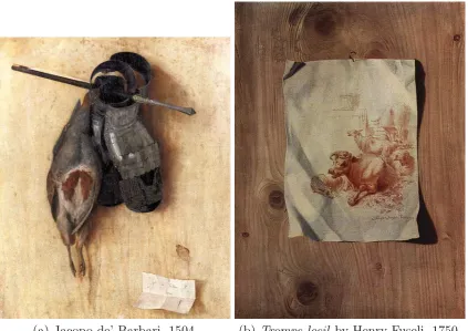
were Parrhasius’s painting. That was one of the first stories of Trompe loeil, literally means ‘deceiving the eye’ or often called ‘trick of the eye’, an art technique that uses realistic imagery to create the optical illusion that
of a partridge, gauntlets, and crossbow bolt (see Figure 1.1(a)), which is
considered as the first small scale Trompe l’oeil painting since antiquity. Another example is shown in Figure 1.1(b) from a painting of Henry Fuseli
(1750).
(a) Jacopo de’ Barbari, 1504. (b) Trompe loeil by Henry Fuseli, 1750. Figure 1.1: Examples of Trompe loeil paintings.
In modern day, Trompe loeil artists create their art by combining tra-ditional techniques with the modern technologies to create more types of
illusions. For example, while the house on 39 George V street, Paris was
being renovated, they printed and hung an interesting artwork on the
scaf-folding to shelter the rehabilitation, which is shown in Figure 1.2(a).
An-other modern Trompe loeil can be seen in Figure 1.2(b), created by Pierre Delavie on facade of the Palais de la Bourse, Marseille, which shows the
Figure 1.2: Examples of modern Trompe loeil paintings.
Trompe loeil not only makes a painting more realistic, but also exploits the techniques that can attack the weaknesses of human visual system,
which can be applied to digital image forensics. Using modern computer
graphics technologies, synthetic scenes, human characters or objects can
be easily created with a very high quality level, which could take years to
artists in classic Trompe loeil. Some examples of computer graphics images are shown in Figure 1.3, in which most of the images are very realistic.
However, these synthetic objects may be used to create situations which
may not be present in real world, and hence raising security risks. For
example in the US, possession of child pornography is illegal since it
im-plies abuse of minors. However, establishing the presence of minors from
the child pornography is challenging on legal ground, as owners of child
pornography can declare the images to be computer generated [36]. This
raise a need of tools able to automatically and reliably discriminate
be-tween CG and natural images in this particular case, and in multimedia
data in general. Hence, many techniques have been proposed to deal with
this problem. A big picture is shown in the next section while the literature
Figure 1.3: Examples of realistic CG photos.
1.1
CG versus Natural Multimedia Data
Discrimina-tion
Detecting computer graphics images has been studied in decades, starting
with classification methods on the type of images [2], mostly for
differen-tiation between graphics and photographs. However, these methods only
targeted to simple graphics images, e.g., cartoons, clip arts or drawing,
which are very different from the photographs. An example of the two
kind of images are shown in Figure 1.4 (a) and (c). Shown in Figure (b) is
an example of a photorealistic CG image, which is almost indistinguishable
by human perception. Only since 2005, with the raising of digital image
forensics, identifying photorealistic computer graphics became attractive
to the multimedia forensic community with many studies on this problem.
(a) A natural photograph. (b) A photorealistic CG image. (c) A graphic image. Figure 1.4: Examples of a photorealistic CG image, a photograph and a graphic image.
• Methods using Recording Devices properties: Photographic images are created in general by a camera, or a scanner. These devices
have various of characteristics that computer could not reproduce in
CG images. Some studies have proposed solutions by analyzing
phys-ical variances in the image (e.g., local patch statistics, fractal and
quadratic geometry, surface gradient) as introduced by Ng. et al. [18]
in 2005. Dehni et al. in 2006 and Khanna et al. in 2008 proposed
methods for solving this problem by evaluating the noise introduced
by the recording device, presented in [9] and [15], respectively. Dirik
et al. [10] and Gallager and Chen [21] introduced methods to
discrim-inate images created by the computer from the ones captured by the
camera by detecting traces of demosaicing and chromatic abberation.
• Methods from Natural Image Statistics: Natural images have some special properties different from the other types of images. One
of it is the sparse distribution of the wavelet coefficients which are
suitably modeled by a generalized Laplacian density [37]. Hence, in
2005, Lyu and Farid proposed a method in [36] to differentiate between
CG and photographic images by estimating statistical differences in
first approaches to this problem. Another method working on wavelet
domain was proposed by Wang and Moulin [56] in 2006, where they
discovered that the characteristic function of the coefficient histogram
of wavelet sub-bands is different for CG and natural images. In 2007,
Chen et al. [5] applied an idea from steganalysis to deal with this
problem on wavelet domain. Another method based on the Benford’s
law on Discrete Cosine Transform is proposed by Xu et al. [58] in
2011.
• Methods using Visual Features: Visual descriptors refer to fea-tures motivated by visual appearance such as color, texture, edge
properties, and surface smoothness [40]. These kind of methods were
used mostly to compared between simple CG with photograph, but
some of them are able to used in detecting highly realistic CG images.
In 2006, Wu et al. [57] proposed a method using several visual clues,
e.g., the number of unique colors, local spatial variation of color and
obtained highly performance on classification. In 2007 Ladonde and
Efros [28] proposed an method based on an assumption that color
composition of natural images is not random, and some compositions
appear more likely than the others. Hence, color compatibility can be
used as discriminate features to distinguish computer graphics from
photographic images. The other method in this group is proposed by
Pan et al. [41] in 2009, in which they used fractal dimension to detect
CG images on the Internet.
• Hybrid and other methods: Sutthiwan et al. proposed two dif-ferent methods in [49, 50] using high dimension feature vectors to
differentiate CG and natural images. Sankar et al. [47] in 2009
intro-duced a method by simply combine the features from various previous
combining various data in a hybrid approach was proposed by
Conot-ter et al. [8]. Recently, Wand and Double [55] and Kee and Farid
[26] proposed methods to measure visual photorealism, which can be
applied to measure the degree of photorealism in an image. However,
such measure is still weak and thus a better measure is required to be
able to differentiate between CG and natural data.
Although many interesting methods have been proposed, most of these
methodologies do not achieve satisfactory performance in the detection of
CG characters. Some examples of human characters are shown in Figure
1.5 where CG and natural faces are almost perceptually indistinguishable.
As a matter of fact, generic methods able to recognize synthetic images
cannot cope with the complexity of this specific problem, which requires
the use of specialized models.
(a) (b) (c) (d)
Figure 1.5: Examples of highly realistic CG characters.
Only the right-most picture is photographic while the first 3 pictures are computer generated.
People are, in many cases, a crucial target for computer graphics
com-munity, hence designers often try their best to create realistic virtual
char-acters. Indeed, computer generated (CG) characters are increasingly used
especially video games. Since the first virtual newsreader Ananova1
intro-duced in 2000, significant improvements have been achieved in both quality
and realism of CG characters, which are nowadays often very difficult to
be distinguished from real ones. Therefore, we consider critical to be able
to distinguish between computer generated and photographic faces in
mul-timedia data. This is the objective of this doctoral study. In the next
section, our proposed solutions and innovation are briefly reported.
1.2
Proposed Solutions and Innovation
The objective of this doctoral study is to develop efficient techniques to
dis-tinguish between computer generated and natural human faces, which can
be used in various contexts, i.e., in both still images and videos, with
differ-ent face poses or in complex situations, e.g., occlusions, differdiffer-ent lightning
conditions or varying facial animations.
Given such requirements, during this doctoral research we contributed
in each application scenario proposing the following approaches :
• Discrimination based on Asymmetry Information (AsymMethod)
Usually, when creating a human face, designers only create a half of the
face, then replicate it to form the other half. Based on that idea, we
proposed a geometric approach supporting the distinction of CG and
real human faces, which exploits face asymmetry as a discriminative
feature. This method can be used without requiring classification tools
and training or combined with existing approaches to improve their
performances.
• Discrimination through Facial Expressions Analysis (Express-Method)
As mentioned, we aim at developing methods not only for still images,
but also for discriminating between CG versus natural subjects in
video sequences. The first method can work also on a single shot,
but when a video source is available, much more information can be
extracted from the data. For instance, CG and real characters can
be discriminated by analyzing the variation of facial expressions in
a video. The underlying idea here is that humans can produce a
large variety of facial expressions with a high range of intensities.
For example, the way a person smiles changes depending on his/her
mood, and hence the same expression is usually produced in similar
but not equal ways. Computer generated faces, instead, typically
follow repetitive patterns, coded into pre-defined models. Therefore,
their variations are not as wide as in real faces. Consequently, a CG
character can be theoretically identified by analyzing the diversity
of facial expressions, through appropriated models. In this method,
face and expression models are created through sets of feature points
identified in critical areas of the face.
To the best of our knowledge, this is the first multimedia forensics
approach that aims at discriminating between CG versus natural
mul-timedia data in video sequences.
• Identifying synthetic facial animations through 3D face mod-els (ModelMethod)
The last method is aim at even more complicated situations, where
characters are moving and turning their faces. The analysis of the 3D
model allows to deal more easily with human faces, which are various,
lightning condition, poses, etc. Therefore, we propose to study the
evolution in chronological order of the 3D model of the analysed
char-acter, assuming that its variations allow to reveal synthetic animation.
Indeed, facial animation following fixed patterns can be distinguished
from natural ones which follow much more complicated and various
geometric distortion, i.e., bigger variations in the 3D model
deforma-tion.
To summarize, we primarily studied geometric-based techniques, which
make use of measurements on human faces. We investigated both image
and video CG versus natural discrimination methods, exploiting knowledge
of objects in the world and of the process of image formation. All of the
proposed methods can be used as standalone methods or combined with
existing approaches.
Following, we briefly present our main contribution to this field:
• CG versus natural human faces: To the best of our knowledge, in the context of Multimedia Forensics, we proposed first approaches to
deal with the problem of differentiate between CG and natural human
faces. This is also the first time the problem of discrimination of CG
versus natural data in videos are considered.
• Geometric-based techniques: the modeling and estimation of ge-ometry is less sensitive to resolution and compression that can easily
confound statistical properties of images and video, i.e., our proposed
methods are robust with different situations.
• Model-based techniques: analyzing through 3D models better fits the analysis of human faces, taking into account their variety,
deforma-bility, diversity of expressions, different poses, as well as the external
1.3
Thesis Structure
The thesis is organized in 5 chapters describing the research field together
with the main objectives of this doctoral study.
Chapter 2 presents an overview on visual realism of computer graphics
and the way synthetic facial animations are created. CG versus Natural
Data Discrimination methods are also deeply reviewed in this chapter.
In Chapter 3, the details of our proposed approaches are presented and
discussed.
Chapter 4 discusses about datasets used in our experiments together
with the experimental results.
Finally, Chapter 5 collects some concluding remarks and discusses the
State of the Art
This chapter presents a concise overview about discrimination between computer generated and natural multimedia data. We also focus our at-tention on visual realism of computer graphics and the way that synthetic facial animations are created.
“Study the past, if you would divine the future.” Confucius
2.1
Visual Realism of Computer Graphics
Since the level of photorealism of a CG product is considered as a value of
success, computer graphics community aware of the important of
photore-alism and its perception. Such studies on perception of photorephotore-alism offer
some hints about the perceptual differences between natural and artificial
multimedia data.
In 1986, Meyer et al. [39] showed to 20 people pairs of CG/natural
Figure 2.1: Examples of the pictures tested from [20].
For each pair of image, the left picture is computer generated while the right one is natural. Figure source: [20].
that test selected the wrong answer.
McNamara [38] in 2005 carried a similar experiment with more complex
CG images. They invited 20 people and show them randomly 10 images,
and asked them to label which images are CG, which are natural. The
results showed that some high quality CG images are undistinguishable
under some conditions of lighting.
More recently, in 2012, Farid and Bravo [20] conducted some
experi-ments that used human face images in different resolution, JPEG
com-pression qualities, and color to explore the ability of human to distinguish
computer generated faces from the natural ones. The CG images are
down-loaded from the Internet. The experiments provided a probability that an
image that is judged to be a photograph is indeed a true photograph,
which has 85% reliability for color images with medium resolution
(be-tween 218×218 and 436×436 pixels in size) and high JPEG quality. The
reliability drops for lower resolution and grayscale images. This work shows
that the CG faces from the Internet are quite distinguishable for human.
However, not all of the selected CG images from this study are highly
re-alistic, for example the CG faces shown in Figure 2.1 are less realistic than
2.2
CG versus Natural Data Discrimination methods
As mentioned in Chapter 1, since about 10 years, the research on
multime-dia forensics have started developing methods to identify photorealistic CG
data, mainly focusing on still pictures. These methods can be grouped into
4 categories, illustrated in Figure 2.2. Details of these groups are presented
in the following sections.
Figure 2.2: State-of-the-art approaches on still images.
The first group uses the recording device properties, mostly by analyzing the noises from the camera sensor, to identify natural images. Second group differentiates the two types of images based on natural image statistics like wavelet coefficients while third group investigates informa-tion from the visual features of the image. The last group contains other and hybrid methods from the first three groups.
2.2.1 Methods from Recording Devices properties
Characteristics of the recording devices and the processing from the
manu-facturer software are often presented in the images, e.g., chromatic
aberra-tion or distoraberra-tions (see Figure 2.2). Further more, most of digital camera
now are using charge-coupled device (CCD) or metal-oxide-semiconductor
(CMOS) sensors, which contain imperfect patterns such as pattern noise,
dark current noise, shot noise, and thermal noise [22]. Such noises are
natural images can be detected based on the analysis on these
character-istics.
In 2005, Ng et al. [18] identified three differences between photographic
images and CG images:
1. Natural images are subject to the typical concave response function
of cameras.
2. Colors of natural images are normally represented as continuous
spec-trum while in CG the color channels are often rendered independently.
3. Natural objects are more complicated while CG objects are normally
modelled by simple and coarse polygon meshes.
Hence, the authors proposed a method using image gradient, Beltrami
flow vectors, and principal curvatures to analyze the three mentioned
dif-ferences, which is summarized in Figure 2.3. Using SVM classification on
the Columbia open data set [17], they achieved an average classification
accuracy of 83.5%.
Dehnie et al. [9] in 2006 indicated that noise patterns, extracted by a
wavelet denoising filter, of natural images is different from the ones in CG
images. Hence, an input image can be classified as CG or natural based
on its correlation to the reference noise patterns. On their own data set,
the method achieved an average accuracy of about 72%.
In 2007, Dirik et al. [10] proposed a method to detect natural images by
analyzing the traces of demosaicking and chromatic aberration. According
to them, in natural images, the changes of the color filter array (CFA) is
smaller, comparing to CG images, when an input image is re-interpolated.
The authors also combined their proposed features with wavelet-based
fea-tures from the method of [36] to obtain a better performance. Their method
achieved an average classification accuracy of about 90% on their own data
Input6Image Fine6Scale Coarser6Scale Compute Rigid Body Moments where Local6Fractal6Dimension 3x36local6patches Local6patch6vectors 64x646pixel6blocks in6scaleVspace where where Beltrami6flow6vector =6Inverse6metric =6magnitude6of6metric where principle6components6of6A Surface6gradient fit6a6linear6function6to6log(F)6vsT6log(t)6plot6and compute6its6slope project6to6a 7Vsphere SVM6Classifier Linear6scale6space To6capture6the6texture complexity6in photographic6images To6capture6the6characteristics of6the6local6edge6profile To6capture6the6shape6of a6camera6response6function To6capture6the6artifacts6due to6the6CG6polygonal6model To6capture6the6artifacts6due to6the6color6independence assumption6in6CG where
Figure 2.3: Schema of the method in [18].
Based on the estimation of the noise pattern of the devices, in 2008,
Khanna et al. presented in [15] a method for discriminating between
scanned, non-scanned, and computer generated images. In this study, the
basic idea is analyzing noises of the scanner from row to row and column to
column, and then combining them with the noise of the camera, calculated
as difference between the de-noised image and the input one. Their idea is
summarized in Figure 2.4. On their own data set, the method achieved an
average accuracy of 85.9%.
Image De-noise filter – Noise pattern
• Mean
• Variance
• Skewness • Kurtosis
Estimate Correlations
Figure 2.4: Schema of the method in [15].
Gallagher and Chen [21] in 2008 demonstrated that the CFA in
original-size natural images can be detected. Firstly, they use a high-pass filter to
highlight the observation that interpolated pixels have a smaller variance
than the original ones. Then, they analyze the variance on green color
channel from the diagonal scan lines since interpolated and original pixels
respectively occupy the alternate diagonal lines. Their method achieved
an average classification accuracy of 98.4% on the Columbia open dataset
2.2.2 Methods from Natural Image Statistics
Natural images have some particular statistical properties that do not
ap-pears frequently in other types of images (computer generated, microscopic,
aerial, or X-ray images). One of the important natural image statistics is
the sparse distribution of the wavelet coefficients: natural images that are
suitably modeled by a generalized Laplacian density [37]. Shown in Figure
2.5 is the wavelet coefficient distributions of the second-level horizontal
subbands, respectively, for a photograph and a computer graphics. Based
on these statistical differences, some methods have been developed to
dis-tinguish CG images from the natural ones.
Figure 2.5: The log-histogram of the first level detail wavelet coefficients.
The wavelet coefficients are computed using Daubechies filters. Dash-line is the least squared fitted generalized Laplacian density. Figure source: [40].
The first approach in this group was introduced in 2005 by Lyu and Farid
[36], which is normally considered as one of the first forensics approaches
in this problem. In this study, the authors use a statistical model on
216-dimensional feature vectors calculated from the first four order statistics of
the wavelet decomposition. The idea of this method is summarized in
Fig-ure 2.6, where input image is first decomposed into three levels, then four
distribution and the linear prediction error distribution are computed for
each subband as features, finally a classic Support Vector Machine classifier
is applied.
They obtained classification rate of 66.8% on the photographic images,
with a false-negative rate of 1.2%. Datasets were collected from the
Inter-net.
12
Linear Predictor
Error statistic (108) Marginal statistic
(108)
H D V
1
2
3
Figure 2.6: Schema of the method in [36].
In a similar way, in 2006, Wang and Moulin [56] used a statistical model
with only 144-dimensional feature vectors achieving slightly better results
with respect to [36]. With less number of features, the computation speed
is about four times faster than that of Lyu and Farid [36]. They also
com-pared indirectly with the method in [18] and the obtained computational
is 70 times faster.
In 2007, Chen et al. [5] applied an idea from steganalysis, in which
they compute three levels of wavelet decomposition on the original and the
sta-tistical moments were computed for each subband which gave 234 features
in total. On a data set expanded from the Columbia open data set [17],
they achieved a classification accuracy of 82.1%.
Xu et al. [58] proposed a method in 2011 based on Benford’s law to
identify natural images. According to the authors, statistics of the most
significant digits extracted from Discrete Cosine Transform (DCT)
coeffi-cients and magnitudes of the gradient image of natural images are different
from CG images. They achieved an accuracy of 91.6% on their own dataset.
2.2.3 Methods from Visual Features
In 2006, Wu et al. [57] used the number of unique colors, local spatial
variation of color, ratio of saturated pixels, and ratio of intensity edges as
discriminative features and used k-NN to classify CG and natural images.
On their own dataset, they achieved an average accuracy of 95%.
In 2007, Lalonde and Efros [28] proposed a method that can identify
composite images by compare the color distribution between the
back-ground and the foreback-ground objects. Their idea is based on an assumption
that color composition of natural images is not random, and some
com-positions appear more likely than the others. This idea can be apply to
differentiate natural images from CG images where color compatibility can
be used as discriminate features. Figure 2.7 illustrates the idea of this
method.
Pan et al. [41] in 2009 proposed a method that use fractal dimension
to analyze the differences between CG and natural images. In particular,
they computed the simple fractal dimensions on the Hue and Saturation
components of an image in the HSV color space as discriminative features.
On their own data set, they achieved an average accuracy of 91.2%, while
Background Color Distribution
Object Color Distribution
Distribution
Comparison Realism score
Figure 2.7: Idea of the method in [28].
2.2.4 Hybrid and Other Methods
In 2009, Sutthiwan et al. [49] considered the JPEG horizontal and vertical
difference images as first-order 2D Markov processes and used transition
probability matrices to model their statistical properties [40]. On their
data set, they achieved the average accuracy of 94.0% by using SVM with
the 324 dimensional feature vectors. An improvement was proposed by
using Adaboost: the number of features is reduced to 150 and the accuracy
increased to 94.2%. In [50], they extended the work by Chen et al. [5].
In this study, they computed the features on the original image, its JPEG
coefficient magnitude image and the residual error. On the same dataset,
they achieved an accuracy of 92.7% by using Adaboost on 450 dimensional
feature vectors.
Sankar et al. [47] in 2009 proposed a hybrid method, in which they
combined all the features from Ianeva et al. [23], Chen et al. [5], Ng et
al. [18], and Popescu and Farid [42]. On the Columbia open data set [17],
they achieved an average accuracy of 90%.
In 2011, Wang and Doube [55] proposed a method to measure visual
roughness, shadow softness, and color variance. However, they evaluated
the realism by comparing the new video games to the old ones, hence such
measure is considered week and better measures are needed.
In 2011, Conotter and Cordin in [8] developed an hybrid method, which
not only exploits the higher-order statistics of [36] but also uses the
in-formation from the image noise pattern (36-dimensional feature vectors
calculated from the PRNU [33] and used also for source identification [7]).
Figure 2.8 illustrate the idea of this method.
Image De-noise filter –
Noise pattern
• Mean
• Variance
• Skewness
• Kurtosis Wavelet-based
features
Figure 2.8: Schema of the method in [8].
We introduced a series of State-of-the-Art methods so far together with
their performances, however, it is not easy to have a direct comparison
since most of the methods were tested on different datasets. Thus, to
summarize all of them, we reported their performance together with the
2.3
Generating Synthetic Facial Animations
Understanding how synthetic faces are generated and animated is the basis
for defining suitable algorithms to model them and to discriminate them
for natural images.
There are studies dating back to the 70s that analyse facial animations
(see for instance [12]). The Facial Action Coding System (FACS) by Ekman
[13] (updated in 2002 [11]) and the MPEG-4 standard [25] are the basis
for most algorithms generating synthetic facial animations. According to
FACS, face muscles are coded as Action Units (AUs) while expressions
are represented as AUs combination. In MPEG-4, explicit movements
of each face point are defined by Facial Animation Parameters (FAPs).
These parameters (FACS of FAPs) make the existed physically-constructed
model more realistic. Thus, synthesis of facial animations is performed
by modeling the facial animations and controlling parameters (Lee and
Elgammal [29]). Linear models, e.g., PCA by Blanz et al. [3] in 1999 and
Chen et al. [4] in 2012, and bilinear models [6][59] have been used for facial
expression analysis and synthesis.
In 2000, Seung et al. [48] discovered that a facial expression sequence lies
on a low-dimensional manifold. Thus, based on that inference, nonlinear
algorithms (e.g., local linear embedding (LLE) proposed by Roweis et al.
[46]) have been applied to find manifold from face datasets. However, these
data-driven approaches fail to find manifold representations where there are
large variations in the expression data by different type of expression and
CG versus Natural Human Faces
In this chapter, we focus on the specific class of images and videos con-taining faces, since we consider critical to be able to discriminate between photographic faces and the photorealistic ones. To this aim, we present new geometric-based approaches relying on face asymmetry information and the repetitive pattern from CG animations. These methods are able to detect CG characters in both still images and videos with high performances.
“Who sees the human face correctly: the photographer, the mirror, or the painter?” Pablo Picasso
As mentioned in Chapters 1 and 2, we primarily studied
geometric-based techniques, which make use of measurements on human faces, to
discriminate between CG and natural faces. We investigated both image
and video CG versus natural discrimination methods, exploiting
knowl-edge of how synthetic animations are created and performed. One of the
advantages of geometric-based techniques is that the modeling and
easily confound statistical properties of images and video. Furthermore,
all of these methods can be used as standalone methods or combined with
existing approaches. In the next sections, details of these methods are
introduced.
3.1
Discrimination based on Asymmetry Information
To the best of our knowledge, when creating synthetic human faces,
design-ers, in most cases, just make a haft of a face and then duplicate it to create
the other one. Then, they often apply post processing to achieve
photore-alistic results but usually not modifying the geometry of the model. Hence,
if a given face present a high symmetric structure, this could be considered
as a hint that it is generated via computer. On the other hand, although
human faces are symmetric, there does not exist a perfectly symmetrical
face, as confirmed by Penton-Voak et al. in [14]. The combination of such
two hints allow us to make the following assumption: the more asymmetric
a human face, the lower its probability to be computer generated. Based
on this assumption, we have developed a method (named AsymMethod) to
compute asymmetry information and thus discriminate between computer
generated and photographic human faces.
Our method contains three main steps as detailed in Figure 3.1: shape
normalization, illumination normalization and asymmetry estimation. First,
in shape normalization step, the input image is transformed into the
‘stan-dard’ shape, i.e. is normalized into the same coordinate system for every
face, in order to make the measurements comparable. Then, in illumination
normalization step, unexpected shadows, which could affect the accuracy
of the measurements, are removed from the normalized face. Asymmetry
measurements which are stable under different face expressions are then
measure-ments, we assign to the given face a probability whether it is computer
generated or not.
Figure 3.1: Schema of AsymMethod.
An example of the process is shown in Figure 3.2, where a) represents
the input image, b) the normalized face, and e) the result after illumination
normalization.
3.1.1 Shape Normalization
We apply the traditional approach from [32] to normalize a shape of a face
in order to have a common coordinate system. This normalization is not
only making the measurements easier, but allows to combine them with
other facial features (e.g., EigenFace or Fisher Face). In particular, two
inner eye-corners, denoted as C1 and C2 and the filtrum, denoted as C3 of
a face are chosen. The given face is then normalized by moving [C1, C2,
C3] into the normalized positions, by the following three steps as follows:
• Step 1. Rotate (C1, C2) into a horizontal line segment.
• Step 2. Apply the shearing transformation that make the philtrum be
on the perpendicular line through the middle point of (C1, C2).
• Step 3. Scale the image that (C1, C2) has the lengthaand the distance
from C3 to (C1, C2) is b. See Figure 3.3 for example.
We used the same normalized values as mentioned in [32], which used
the fix values of the special points: C1 = (40, 48), C2 = (88, 48), and C3 =
(64, 84). The (0, 0) is the top-left corner. Figure 3.2 b) shows an example
(a) (b)
(c) (d)
(e)
(f) (g)
Figure 3.2: Face asymmetry estimation.
Figure 3.3: Face normalization via inner eye-corners and a philtrum.
Figure source: [32]
3.1.2 Illumination Normalization
Illumination causes most challenging problems in facial analysis.
Asym-metry measure is calculated based on the intensity of the face image, thus,
the shadows, which are usually quantized as low value regions, play an
important role. However, what we need is the information of the face
structure, without any effects from shadows or unexpected lighting
illumi-nation. Hence, illumination normalization is required in order to enhance
the accuracy of the asymmetry measurements.
We apply the approach presented by Xie et al. in [19]. The basic idea is
to use the albedo of large scale skin and background, denoted as Rl(x, y)
to split the face image I into large-scale and small-scale components. Based on Lambertian theory, we have:
apply a transformation to overcome this issue as follows:
I(x, y) = R(x, y)L(x, y) =
R(x, y)
Rl(x, y))
(Rl(x, y)L(x, y)) (3.2)
= ρ(x, y)S(x, y)
where ρ contains the intrinsic structure of a face image, and S contains the extrinsic illumination and the shadows, as well as the facial structure. ρ
and S are called small-scale features and large-scale features, respectively. In order to split the image into large-scale and small-scale, the
Log-arithm Total Variance (LTV) estimation is used. This estimation is
in-troduced in [16] and is the best method to extract illumination-invariant
features so far. After splitting the image I into ρ and S, smoothing filter, which is also introduced in [19], are required to be applied on ρ in order to remove unexpected effects from the decomposition in (3.2).
An example of this step is shown in Figure 3.2 where c) and d) represent
the large-scale and small scale components, respectively, after applying
LTV on the image b). The illumination normalized result is shown in e).
3.1.3 Asymmetry Evaluation
In order to estimate asymmetry, we use the measure introduced by Liu
et al. in [32], which is less depend on face expressions. Let us denote
the density of the image with I, and the vertically reflected of I with I0. The edges of the densities I and I0 are extracted and stored in Ie and
Ie0, respectively. Two measurements for the asymmetry are introduced as follows:
Density Difference (D-Face):
Edge orientation Similarity (S-Face):
s(x, y) = cos θIe(x,y),I0
e(x,y)
(3.4)
where θIe(x,y),I0
e(x,y) is the angle between the two edge orientations of
images Ie and Ie0, at position (x, y). Figure 3.2 (e) shows the estimated
frontal face resulting from the illumination normalization step. In Figure
3.2 (f) and (g) the D-Face and S-Face are shown, respectively.
Based on these measurements, we can estimate the asymmetry of a given
face photo since the higher the value ofD-Face, the more asymmetric is the face, and the higher the value of S-face, the more symmetric the face. The total difference of D-Face and total dissimilarity of S-Face are calculated as follows:
D = P
x,y∈Ωd(x, y)
η1
; (3.5)
S = 1−
P
x,y∈Ωs(x, y)
η2
(3.6)
where η1, and η2 are the normalized thresholds, which scale D and S
into (0; 1), and Ω is the estimated region. Since our images are normalized
to the fixed size 128× 128, and Ω is fixed as in [32], both thresholds η1,
and η2 are fixed.
Finally, we assign to image I an exponential probability to be computer generated, as follows:
P = λe−λ
√
D2+S2
(3.7)
where λ is a constant (we use λ = 1.0). If P is over a threshold τ, I is classified as a computer generated human face (we use τ = 0.5).
The results, which are introduced in details in Chapter 4, show that
AsymMethod can be used as a stand alone method or in combination with
In the next section, ExpressMethod, which discriminate between CG and
natural faces in videos or sequences of faces, is presented.
3.2
Discrimination through Facial Expressions
Anal-ysis
In order to deal with more complicated situations in videos or sequences
of images, we proposed a second method, namely ExpressMethod, to
dis-tinguish between CG and real characters by analysing facial expressions.
The underlying idea is that facial expressions in CG human characters
follow a repetitive pattern, while in natural faces the same expression is
usually produced in similar but not equal ways (e.g., human beings do not
always smile in the same way). Our forensic technique take as input
var-ious instances of the same character expression (extracting corresponding
frames of the video sequences) and determine whether the character is CG
or natural based on the analysis of the corresponding variations. We show
that CG faces often replicate the same expression exactly in the same way,
i.e., the variations is smaller than the natural ones, and can therefore be
automatically detected.
Our method contains five steps as detailed in Figure 3.4:
• From a given video sequence, frames that contain human faces are
extracted in the first step A.
• Then, in step B, facial expression recognition is applied in order to
recognize the expressions of the faces. Six types of facial expressions
are used in this step, following the six universal expressions of Ekman
(happiness, sadness, disgust, surprise, anger, and fear) [13] plus a
‘neutral’ one. Based on the recognition results, faces corresponding
steps. Notice that the ‘neutral’ expressions are not considered, i.e.,
faces showing no expression are not taken into account for further
processing.
• In the next step C the Active Shape Model (ASM), which represents
the shape of a face, is extracted from each face. In order to measure
their variations, all shapes have to be comparable.
• In step D, each extracted ASM is then normalized to a standard shape.
After this step, all ASM shapes are normalized and are comparable.
• Finally, in step E, differences between normalized shapes are
anal-ysed, and based on the variation analysis results, the given sequence
is confirmed to be CG or natural.
The right part of Figure 3.4 shows an illustration of the analysis
pro-cedure on happiness expression. Seven frames that contain faces are
ex-tracted in step A. Then, facial expression recognition is applied in step B
and three happy faces are kept. For each face, the corresponding ASM
model, which is represented by a set of reference points, is extracted in
step C. Then, each model is normalized to a standard shape, step D. All
normalized shapes are then compared together in step E, and based on the
analysis results the given character is confirm as computer generated since
the differences between the normalized shapes are small (details about the
variation analysis are given in the following Subsection 3.2.5).
3.2.1 Human Faces Extraction
Face detection problem has been solved with the Viola-Jones method [54],
which can be applied in real-time applications with a high accuracy. In
this step, we reuse this approach to detect faces from video frames, and
Disgust Happy Surprise Happy Disgust Happy Neutral Human Faces
Extraction
Facial Expression Recognition
Active Shape Model Extraction
Variation Analysis Normalized Face Computation
RESULT INPUT
?
A
B
C
D
E
Figure 3.4: Schema of ExpressMethod.
method can be found in [53] and [54]. It is worth mentioning that in this
first work we do not face the problem of face recognition, thus assuming
to have just a single person per video sequence (the analysed character).
3.2.2 Facial Expression Recognition
Facial expression recognition is a nontrivial problem in facial analysis. In
this study, we applied an EigenFaces-based application [45] developed by
Rosa for facial expression recognition. The goal of this step is to filter
out the outlier expressions and keep the recognized ones for further steps.
Notice that this application associates an expression to a given face without
requiring any detection of reference points. In Figure 3.4 an example of
results of this application is shown with 7 faces (3 happy, 2 disgust, 1
surprise and 1 neutral).
3.2.3 Active Shape Model Extraction
Input images for this step are confirmed to have the same facial expression
of the same person, thanks to the preprocessing in the first two steps. In
order to extract face shapes, which are used in our analysis, an alignment
method is applied. In this step, we follow the Component-based
Discrim-inative Search approach [31], proposed by Liang et al. The general idea
of this approach is to find the best matching from the mode candidates,
where modes are important predefined points on face images (e.g., eyes,
nose, mouth) and are detected from multiple component positions [31].
Given a face image, the result of this step is a set of reference points,
representing the detected face. In Figure 3.6 (a) an example of this step
is shown, where the right image shows reference points representing the
face in the left image. In this method, the authors exploit the so called
Figure 3.5: The 87 points of Active Shape Model (ASM).
Figure source: Microsoft Research Face SDK.
example of this step on a CG face is also reported in Figure 3.6 (c), where
the left image shows the synthetic facial image and the right one shows the
corresponding ASM.
3.2.4 Normalized Face Computation
ASM models precisely and suitably represent faces, but they are
incom-parable since faces could be different in sizes or orientations. They need
to be normalized in order to be comparable. In this step, we apply the
traditional approach from [32] to normalize a shape of a face in order to
have a common coordinate system. This normalization is an affine
trans-formation used to transform the reference points into fixed positions. Since
eye inner corners and the philtrum are stable under different expressions,
these points have been chosen as reference points. Shown in Figure 3.5,
the reference points number 0 and 8 are two inner eye corners. The last
reference point, the philtrum, can be computed via the top point of outer
as follows:
pphiltrum =
p41+p42
2 +p51
2 (3.8)
where p41, p42, and p51 are the reference points on the extracted ASM.
After computing the three reference points, each ASM model is
nor-malized by moving {p41, p42, pphitrum} into their normalized positions, as
follows: (i) rotate the segment [p41, p42] into an horizontal line segment;
(ii) shear the philtrum to be on the perpendicular line through the middle
point of [p41, p42]; and finally (iii) scale the image so that the length of
seg-ment [p41, p42] and the distance from pphiltrum to [p41, p42] have predefined
fixed values (see [32] for more details). An illustration of this normalization
is shown in Figure 3.3 in Section 3.1.
Shown in Figure 3.6 (b) and (d) are examples of the normalized faces
after Face Normalization step. The left images show the normalized faces
and the right ones show the normalized reference points.
3.2.5 Variation Analysis
In this step, differences among normalized ASM models are analysed in
order to determine if a given character (and therefore the corresponding
set of faces) is CG or real. We analyse the differences as described in the
following paragraphs.
First, the distance di,p of each reference point p on a model i to the
average of all points p of all models is calculated as:
di,p = k(x, y)i,p−(x, y)pk (3.9)
where (x, y)i,p is the position of the reference point p on the model i;
(x, y)p = N1 N
P
i=1
(x, y)i,p, where N is the number of normalized ASM models;
Figure 3.6: Examples of computed ASM and normalized ASM.
Depending on the facial expression ξ (among six universal expressions), a subset Sξ of reference points (not all 87 points) are selected for the
anal-ysis. For example, with the happy facial expression (ξ = 1) only reference points from 0 to 15 and from 48 to 67, which represent the eyes and the
mouth, are considered, i.e., S1 = {0,1,2..15,48,49, ..,67}. The subsets are
selected based on our experiments and suggestions from EMFACS [13], in
which a facial expression is represented by a combination of AUs codes.
Shown in Table 3.1 are the reference points selected in our method and the
correspondent AUs codes from EMFACS. Some explanations of the AUs
codes are also listed in Table 3.2. Full codes in EMFACS could be seen in
[13].
Table 3.1: Expressions with Action Units and correspondent ASM points
ξ Expression Action Units (AUs) Reference Points (Sξ)
1 Happiness 6+12 S1 ={0−15,48−67}
2 Sadness 1+4+15 S2 ={0−35,48−57}
3 Surprise 1+2+5B+26 S3 ={16−35,48−67}
4 Fear 1+2+4+5+20+26 S4 ={16−35,48−57}
5 Anger 4+5+7+23 S5 ={0−64}
6 Disgust 9+15+16 S6 ={0−15,48−67}
Two main properties are taken into account in this analysis: mean and
variance, calculated as their traditional definitions:
µp =
1
N
N
X
i=1
di,p, and σp =
1
N
N
X
i=1
||di,p−µp||2 (3.10)
whereµp and σp are the mean and variance of all distancesdi,p at reference
point p over all models.
The given set of models on expressionξ is confirmed to be CG or natural by comparing the Expression Variation Value EV Vξ to the threshold τξ.
Table 3.2: Meaning of the AUs. AU Number FACS name
1 Inner Brow Raiser 2 Outer Brow Raiser 4 Brow Lowerer 5 Upper Lid Raiser1 6 Cheek Raiser 7 Lid Tightener 9 Nose Wrinkler 12 Lip Corner Puller 15 Lip Corner Depressor 16 Lower Lip Depressor 20 Lip Stretcher
23 Lip Tightener 26 Jaw Drop
The value of EV Vξ is computed as follows:
EV Vξ = αξ
1
|Sξ|
P
p
µp
λ1,ξ
+ (1−αξ)
maxp{σp}
λ2,ξ
(3.11)
where αξ is a weighted constant, αξ ∈ [0; 1]; λ1,ξ and λ2,ξ are the
normaliza-tion values used to normalize the numerators into [0; 1]. In our experiments
αξ are set to 0.7 for ξ = 1, ...,6.
EV Vξ is then compared with τξ, recognizing the character corresponding
to the set of faces as CG if EV Vξ < τξ, natural otherwise.
Shown in Figure 3.7 are the mean values, corresponding to all 87 ASM
points, for the sadness expression (ξ = 2) analysed on the two set of images shown in Figures 3.7(a) and 3.7(b). The horizontal axis represents p, from 1 to 87, while the vertical axis shows the value of µp. Since the facial
expression is sadness (ξ = 2), only the values from µ0 to µ35 and from
µ48 to µ57 are considered (see the selected reference points in Table 3.1).
In this example, the Expression Variation Value EV V2 of the CG face is
(a) Sadness human faces.
(b) Sadness CG faces.
0 10 20 30 40 50 60 70 80 90 0
0.5 1 1.5 2 2.5 3 3.5
Computer Generated Natural
Differences on the mean of ASM points between (a) and (b).
Figure 3.7: Example of differences on the mean of ASM points on sadness expression.
happiness faces is shown in Figure 3.8.
(a) Happiness human faces.
(b) Happiness CG faces.
Differences on the mean of ASM points between (a) and (b).
with the goal of keeping the miss classification as small as possible.
In the next section, our last proposed method is presented, which can be
applied to more complex situations and animations without using different
configurations while ExpressMethod requires the analysis of different sets
of points for each single expression.
3.3
Identifying Synthetic Facial Animations through
3D Face Models
ModelMethod is a model-based method which allow to deal with natural
behaviours of represented facial animation, where characters are moving
and turning their faces. Computer generated facial animations are usually
created by deforming a face model according to given rules or patterns.
Typically, the deformation patterns are pre-defined and contain some
pa-rameters to rule the intensity of the expression. Also natural expressions
are similar to one each other to some extent, due to physical limitations
and personal attitudes, although in this case the variety of the expressions
is much higher, taking into account asymmetries, different grades, bland
of various sentiments, context, and so on.
What we propose here is to define a metric which we can be used to
measure the diversity in animation patterns, in order to assess if the
rel-evant video shows a synthetic characters or a human being. The idea is
that a high regularity of the animations suggests that the face is computer
generated, while a high variety is typically associated to natural images.
The proposed method associates a 3D model to the face to be analyzed
and maps the various instances of the face in the video to the model,
ap-plying appropriate deformations. Then, it computes a set of parameters
associated to the relevant deformation patterns. Finally, it estimates the
thus leading to the classification of the face in synthetic or natural.
The choice of using a face model instead of working directly on the
image is motivated as follows:
• The face model is less dependent on changes of the pose;
• Meaningful information about the whole face is taken into account
instead of separate feature points;
• The face model reconstruction does not require all facial feature points,
which are not always available due to occlusion or lighting condition,
and can be computed for many more instances of the face within the
video.
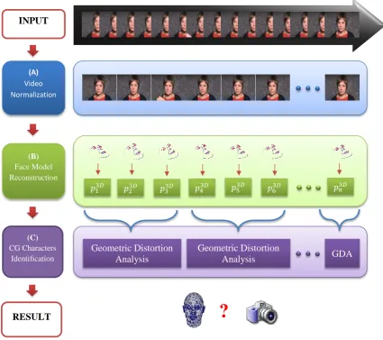
The proposed method, illustrated in Figure 3.9, consists of 3 main steps
as below:
• (A) Video normalization: the video sequence is brought to stan-dard parameters in terms of resolution and framerate, so as to
min-imize possible alterations of the model caused by different video
for-mats;
• (B) Face model reconstruction: facial feature points, which rep-resent the face shape, are extracted via Active Shape Model (ASM)
and a face form in 3D is reconstructed by modelling a neutral shape
to best approximate the extracted ASM;
• (C) CG characters identification: the sequence of actualized 3D face models is represented by applying a Principle Component
Analy-sis (PCA), and the variations of the obtained feature vectors are used
(A) Video Normalization
(B) Face Model Reconstruction
(C) CG Characters
Identification
RESULT INPUT
?
𝑝13𝐷 𝑝
23𝐷 𝑝33𝐷 𝑝43𝐷 𝑝53𝐷 𝑝63𝐷 𝑝𝑛3𝐷
Geometric Distortion Analysis
Geometric Distortion
Analysis GDA
Figure 3.9: Schema of ModelMethod.
3.3.1 Video Normalization
Since the proposed method applies to any kind of video source, first of all
we normalize the source to a standard format to avoid variations in the
model due to the characteristics of the video. The frame rate is therefore
reported in the range 10-12 frames/second, which are largely sufficient to
capture all the significant expression variations in a human face (noticed
that the human visual system can process 10 to 12 separate images per
second [43]).
To perform this operation, a distance measure Df(Fi, Fj) between face
models in frame Fi and frame Fj is defined and computed by exploiting
three special feature points:
Df(Fi, Fj) =
1 3
X
k∈K
||ρki −ρkj|| (3.12) where || · || is Euclidean distance, ρki and ρkj are the spatial coordinates of point k on the face in frame Fi and frame Fj and K = {left-eye inner
corner, right-eye inner corner, philtrum} (see these points in Figure 3.3).
For every second, i.e., for every i and j such that ||i −j|| = 1 second, if Df(Fi, Fj) is smaller or equal to a threshold T, M frames between Fi
and Fj are grabbed. In our experiments, with T equal 8, 10, and 12, the
number of frames grabbed M are 10, 11, and 12, respectively. Notice that there are no videos with Df(Fi, Fj) > 12 in our experimental datasets. As
to the spatial resolution, each face is analyzed in a resolution of 400×400.
We choose two inner corners and a philtrum due to their stability under
different expressions and lighting conditions [32]. Therefore, distances of
these points can be considered as a measure of speed of the head movement.
This step helps to convert an input video into a homogeneous series of
3.3.2 Face Model Reconstruction
In order to reconstruct the face model from a 2D input image, we apply the
method from [4]. After building a reference 3D model, this method adapt
this reference model to the 2D image through an optimization procedure.
To build the reference 3D model, Algorithm 1 is applied on a training
set of 3D images, to construct a normalized mean shape S3D which can be considered as a general 3D face model, and the corresponding eigenvectors
matrix ϕ3D, which can be used to transform a given 3D shape into the 3D face model. This normalized mean shape S3D and the eigenvectors matrix
ϕ3D are called 3D Point Distribution Model (PDM). Notice that the PDM is built only once and can be applied to different faces in different videos.
By using the PCA, new shapes can be expressed by linear combinations
of the training shapes [27], hence the normalized mean shape S3D can be deformed (larger eyes, wider chin, longer nose, etc.) to best fits the input
faces.
Given a PDM, we now have to approximate it to all instances of faces
output of step (A). In order to reconstruct the face model from a 2D input
image, we have to project the 3D PDM into 2D space. This could be done
through an optimization procedure, which is summarized as Algorithm 2.
The main idea is to perform the optimization process on a single instance
each time: face pose is estimated based on the generated shape, then
based on the new computed pose, the new face shape is re-estimated, and
so on, i.e., either shape or pose is estimated each time based on the other
information. Thus, step (B) will produce all the information needed to
map the set of 2D faces into the corresponding set of 3D face models.
Notice that differently from [4], the ASM points for each 2D face s2D
are extracted by using Luxand FaceSDK [34], which able to extract 66
Algorithm 1 Compute 3D Point Distribution Model (PDM)
Input: n different shapes of faces {s3D
1 , s32D, . . . , sn3D}, where s3iD = {x1
i, yi1, zi1, x2i, yi2, zi2, . . . , xdi, ydi, zdi}, where d is the number of ASM points and
(xki, yik, zik) is the spatial position of point kth on face ith.
Output: A normalized mean shape S3D and the corresponding eigenvectors matrixϕ3D
of the training faces. Method: (inspired from [4])
1: Normalize all face shapes: all the points are scaled into [-1, 1]:
Si3D ←N ormalize3D(si3D),i= 1,2, ..., n.
2: Compute the mean shape: S3D ← 1
n
Pn
i=1S 3D i
3: repeat
4: for each normalized shape S3D
i do
5: Find rotation matrix Ri and translation vector ti to transform Si3D into S
3D
.
6: S3D
i ←Ri(Si3D) +ti.
7: end for
8: Re-compute the mean shape: S3D ← 1
n
Pn
i=1S 3D i
9: until convergence.
10: Apply Principal Component Analysis (PCA) to all normalized shapes Si3D, i =
1,2, ..., nto have the eigenvectors matrix ϕ3D.
(ox, oy)), the rotation matrix R and the translation vector t in equation
(3.13) and (3.14), are represented as a single camera projection matrix,
and hence can be jointly approximated. They can be decomposed from
the camera projection matrix by using the method in chapter 6, section
6.3.2 in [52].
Given the 3D PDM defined exploiting Algorithm 1, we report in Figure
3.10 an example 3D face reconstruction (step B). The left picture shows
an example of 2D facial features extraction using Luxand FaceSDK [34].
Algorithm 2 is then applied to the extracted 2D points, and the 3D shape
and model are reconstructed, as shown in the right picture.
The accuracy of step (B) is critical for the following step (C) and will
Algorithm 2 Extract pose and face parameters (from [4])
Input:
• A shape in 2D: s2D = {x1, y1, x2, y2, . . . , xd, yd}, where d is the number of ASM points and (xk, yk) is the spatial position of point kth on the input face.
• A PDM (S3D and ϕ3D).
Output: The face model p3D, rotation matrix R and translation vector t.
Method:
1: Normalize the face shape: all the points are scaled into [-1, 1]: S2D ← N ormalize2D(s2D)
2: p3D ←0.
3: while p3D, R, and t do not converge do
4: Compute R and t by solving
Err = S
2D −P(R(S3D +ϕ3Dp3D) +t) 2 (3.13) using Zhang’s method [60], P is the projection transformation. A 3D point (xi, yi, zi)T is projected by P into 2D space as follows:
P xi yi zi = f zi xi yi + ox oy (3.14)
wheref is the focal length, and (ox, oy) is the principal point location on 2D image.
5: Compute the new face: S∗3D ←R(S3D +ϕ3Dp3D) +t
6: Generate the ideal 3D shape S03D: S03D ← x and y values from S2D and z values fromS∗3D.
7: Recompute p3D from S03D:
p3D = (ϕ3D)T(R−1(S03D−t)−S3D).

![Figure 2.3: Schema of the method in [18].](https://thumb-us.123doks.com/thumbv2/123dok_us/540219.2053520/31.595.111.528.164.597/figure-schema-of-the-method-in.webp)
![Figure 2.4: Schema of the method in [15].](https://thumb-us.123doks.com/thumbv2/123dok_us/540219.2053520/32.595.62.508.291.501/figure-schema-of-the-method-in.webp)
![Figure 2.6: Schema of the method in [36].](https://thumb-us.123doks.com/thumbv2/123dok_us/540219.2053520/34.595.109.460.233.494/figure-schema-of-the-method-in.webp)
![Figure 2.8: Schema of the method in [8].](https://thumb-us.123doks.com/thumbv2/123dok_us/540219.2053520/37.595.97.542.328.554/figure-schema-of-the-method-in.webp)