Doctoral School in Environmental Engineering
Assessing solar radiation components
over the alpine region
Advanced modeling techniques for
environmental and technological applications.
Mariapina Castelli
Doctoral thesis in Environmental Engineering, XXVI cycle Faculty of Engineering, University of Trento
Academic year 2014/2015 Supervisors:
Prof. Dino Zardi, University of Trento
Dott. Marcello Petitta, European Academy of Bolzano
University of Trento Trento, Italy
Acknowledgments
Contents
Abstract 15
1 Introduction 17
1.1 Aim of the thesis . . . 17
1.2 Outline of the thesis . . . 18
1.3 The importance of solar radiation data . . . 19
1.4 Ground based measurements of radiation . . . 22
1.5 Data-driven decomposition methods . . . 23
1.6 Radiative Transfer Modeling . . . 23
1.7 Remote sensing of solar radiation . . . 25
2 Fundamentals of solar radiation 27 2.1 Concepts and definitions . . . 27
2.2 Solar radiation at the top of the atmosphere . . . 29
2.3 Atmospheric absorption and scattering . . . 32
2.4 The effect of the Earth’s geometry . . . 35
2.4.1 Surface albedo . . . 37
3 Ground based measurement of solar irradiance in South Tyrol 39 3.1 Measurement of radiation components . . . 39
3.2 The ground network of pyranometers in South Tyrol . . . 45
4 Estimation of diffuse radiation with decomposition models and
artificial neural networks 51
3
4.1 Introduction . . . 51
4.2 Input data . . . 52
4.3 The model of Reindl . . . 54
4.3.1 Validation . . . 54
4.4 The model of Boland-Ridley-Laurent (BRL) . . . 55
4.4.1 Validation . . . 57
4.5 The logistic model . . . 57
4.5.1 Validation . . . 59
4.6 Artificial Neural Networks (ANN) . . . 59
4.6.1 Method . . . 63
4.7 Validation of logistic and ANN models . . . 66
4.8 Conclusions . . . 66
5 Atmospheric radiative transfer 69 5.1 The equation of radiative transfer . . . 69
5.2 The radiative transfer model libRadtran . . . 73
5.3 Applications: modeling the radiative forcing of measured aerosol profiles . . . 75
6 Radiative forcing and heating rate of measured vertical profiles of black carbon aerosol 77 6.1 Abstract . . . 77
6.2 Introduction . . . 78
6.3 Experimental . . . 81
6.3.1 Sampling sites . . . 81
6.3.2 Vertical profile measurements . . . 82
6.3.3 Aerosol Optical Properties . . . 87
6.3.4 Radiative transfer and heating rate calculations . . . 96
4
6.4.1 Vertical profile measurements . . . 100
6.4.2 Validation of aerosol optical properties . . . 107
6.4.3 Vertical profiles of aerosol optical properties . . . 114
6.4.4 DRE and heating rate profiles . . . 117
6.5 Conclusions . . . 122
7 Remote sensing of solar radiation 125 7.1 Basics of satellite remote sensing . . . 125
7.2 Meteosat geostationary satellites . . . 130
7.3 The method HELIOSAT . . . 133
7.4 The algorithm HelioMont . . . 135
7.4.1 Cloud Mask . . . 137
7.4.2 Clear-sky radiation . . . 141
7.4.3 All-sky radiation . . . 143
8 Validation and improvement of the algorithm HelioMont 149 8.1 Abstract . . . 149
8.2 Introduction . . . 150
8.3 Data and method . . . 151
8.3.1 The method HelioMont for deriving SIS from MSG data . . 153
8.3.2 Ground based radiation data . . . 154
8.3.3 Satellite and ground based atmospheric data . . . 156
8.4 Results . . . 157
8.4.1 Validation of all-sky SIS, SISDIF and SISDNI . . . 157
8.4.2 Validation of the mean diurnal cycle of SIS, SISDIF and SISDNI . . . 162
8.4.3 Validation of SIS, SISDIF and SISDNI under different sky conditions . . . 163
8.5 Modeling the effect of aerosols . . . 168
8.5.1 MACC aerosol data . . . 172
8.6 Conclusions . . . 173
8.7 Outlook . . . 176
9 Conclusions and outlook 179 9.1 Achievements . . . 179
9.2 Outlook . . . 181
List of Figures
2.1 Spectrum of electromagnetic radiation. From Wikipedia (2015). . . 282.2 Geometry of radiative transfer in polar coordinates (Liou, 2002) . . 29
2.3 The 2000 American Society for Testing and Materials (ASTM) E-490 AM0 (air mass 0) Standard Extraterrestrial Spectrum superim-posed to the blackbody emission curve at 5782 K . . . 31
2.4 Solar irradiance spectrum at the top of the atmosphere and at the surface for a solar zenith angle of 60◦, under clear-sky conditions (Liou, 2002). . . 34
3.1 View-limiting geometry of a pyrheliometer (Kipp&Zonen, 2008). The opening angle is 2×arctan(R/L) and the slope angle isarctan(R− r)/L. . . 40
3.2 Details of a pyranometer (Kipp&Zonen, 2013). . . 41
3.3 Shading devices for intercepting beam irradiance and measuring dif-fuse irradiance with a pyranometer (Kipp&Zonen, 2013). . . 42
6 3.4 Pyranometers of the province of Bolzano which were installed after
2009. . . 47
3.5 Histogram of the distance between measurement stations in South Tyrol. . . 47
3.6 Monthly averages of global solar irradiance in South Tyrol at sta-tions installed after 2009. The shaded area represents the standard deviation of the original 10 minute data. . . 48
4.1 Performances of the model of Reindl-Helbig at Bolzano (a, b), Davos (c, d) and Payerne (e, f). The plots on the left hand side show kd against kt, while the plots on the right hand side show the scatter-plot of modeled diffuse irradiance against measured diffuse irradi-ance and also include the statistical performirradi-ances, in terms of MAB, MBD and RMSE, in Wm−2. . . 56
4.2 Performances of the model of Boland-Ridley-Laurent at Bolzano (a, b), Davos (c, d) and Payerne (e, f). The plots on the left hand side show kd against kt, while the plots on the right hand side show the scatterplot of modeled diffuse irradiance against measured diffuse irradiance and also include the statistical performances, in terms of MAB, MBD and RMSE, in Wm−2. . . 58
7
4.4 Performances of the logistic model with coefficients averaged over the ones tuned for Bolzano (a, b), Davos (c, d) and Payerne (e, f). The plots on the left hand side show kd against kt, while the plots on the right hand side show the scatterplot of modeled diffuse irradiance against measured diffuse irradiance and also include the statistical performances, in terms of MAB, MBD and RMSE, in Wm−2. . . . 61
4.5 Performances of the logistic model, with coefficients derived from Bolzano, Davos and Payerne, at Weissfluhjoch. The plot on the left hand side showskd againstkt, while the plot on the right hand side shows the scatterplot of modeled diffuse irradiance against measured diffuse irradiance and also include the statistical performances, in terms of MAB, MBD and RMSE, in Wm−2. . . . 67
6.1 (a) Location of the three sampling sites: Terni in central Italy (Terni Valley), Milan in northern Italy (Po Valley) and Merano in the Alpine region (between Passiria and Val Venosta valleys); (b) the tethered balloon flying over Merano with the instrumentation package. 83 6.2 Vertical profiles measured over TR on 28 January 2010 (13:45-14:26
UTC): (a) BC (blue line) and aerosol (green line, OPC total particle-number concentration); (b) potential temperature (red line) and relative humidity (light blue line). . . 101 6.3 Linear correlation between the mixing height derived from each
ver-tical profile of aerosol concentration (p-MH) temperature (T-MH) and relative humidity (RH-MH). . . 102 6.4 The statistical mean profiles of both BC and aerosol number
8 6.5 Aerosol chemical composition determined BMH and AMH for TR,
MI and ME. Data shown are the respective aerosol mass fractions of each individual aerosol species. . . 105 6.6 (a) Aerosol phase function (P(θ)) along the atmospheric column
over MI and the one obtained at AERONET Ispra; (b) linear cor-relation between the babs determined from Mie calculations and the one measured by the micro-AethRAE51 along vertical profiles for
TR, MI and ME (the 1 : 1 black line is also plotted). . . 114 6.7 Vertical profiles of aerosol optical properties (babs, bsca, bext and
SSA) at 675 nm over (a) TR, (b) MI and (c) ME. . . 115
6.8 ∆DREAT M (a), ADRE (b) and HR (c) calculated for each site and broad-range altitude layers: BMH (from ground to MH), AMH (from MH to 1 km) and FT (> 1 km). . . 118 6.9 Continuous vertical profiles of ADRE over TR (a), MI (b) and ME
(c). . . 120 6.10 Continuous vertical profiles of HR over TR (a), MI (b) and ME (c). 121
7.1 First natural-color RGB image of the Earth acquired by the MSG-2 satellite on MSG-25 January MSG-2006. Low clouds are white, vegetation is green, deserts are reddish brown, and snow cover and high ice clouds are cyan. . . 131 7.2 The classification tree (left) versus the aggregated rating (right)
cloud masking method, from St¨ockli (2013b). . . 136
9
8.2 Monthly averages of satellite and ground based irradiance in Bolzano (2011), Davos (2011) and Payerne (2004-2009). The local minima of global and direct normal irradiance in June and July in Bolzano and Davos are due to the high percentage of cloudy days. In Bolzano no data were available for January because the radiometers were installed in February 2011. In Figure 8.2c the error bars represent the inter-annual standard deviation of monthly averages of satellite and ground measurements. Given its low variability from year to year, the climatology of SISDIF can be considered representative of the single years. . . 161
8.3 Mean diurnal cycle of MBD of irradiance components in Bolzano and Davos. Only the data between 8 a.m. and 4 p.m. are repre-sented because they are descriptive of the entire dataset, in fact in the remaining hours, during autumn and winter, the sun is below the local horizon. . . 163
8.4 Mean diurnal cycle of MBD of irradiance components in Payerne. Only the data between 8 a.m. and 4 p.m. are represented because they are descriptive of the entire dataset, in fact in the remaining hours, during autumn and winter, the sun is below the local horizon. The error bars represent the standard deviation of the daily cycle of MBD in the 6 years 2004-2009. . . 163
8.6 Monthly averages of satellite and ground measurement of diffuse irradiance in Bolzano (2011), Davos (2011) and Payerne (2004-2009) under clear-sky conditions. Only the time interval between 10 a.m. and 2 p.m. was considered in the averaging of cloud mask and irradiance because in these hours most of the irradiance is available. 166
8.7 Summary of the input used for performing RTM simulations in Bolzano and Davos. . . 170
8.8 Hourly averages of RTM simulations, ground measurements, and satellite retrieval of diffuse irradiance in Bolzano and Davos. MAB and MBD refer to the comparison between RTM simulations and ground measurements. Only the hours between 10 a.m. and 2 p.m. were considered. The daily averages of AOT, SSA and water va-por column amount measured by AERONET sun photometers were used as input for RTM simulations. The vertical dashed lines sepa-rate the days from each other. On the x axis there is the sequence cloud-free hours (40 for Bolzano, 45 for Davos) for which averages were computed. The surface albedo was set to 0.1 in Bolzano and 0.4 in Davos. . . 171
8.9 Comparison between daily AOD values obtained by different models and measurement instruments at Bolzano, during August 2011. For AERONET and MACC data, daily averages were computed from the original dataset, while MODIS data are available daily, and the Kinne database includes monthly climatologies. . . 173
8.10 Comparison between hourly averages of diffuse irradiance simulated by libRadtran with MACC aerosol data, estimated by HelioMont, and measured by ground-based instruments. . . 174
11
List of Tables
3.1 Name and altitude of the ground measurement stations which are mapped in Figure 3.4. . . 46
4.1 Parameter of the logistic function for Bolzano, Davos and Payerne. 59 4.2 Combinations of input parameters used for training the network. . . 64 4.3 Correlation coefficient, MAB and MBD for the network structures
which gave the best results. . . 64 4.4 Correlation coefficient, MAB and MBD, in terms of diffuse
irradi-ance, for the network structures which gave the best results. The results in terms of diffuse fraction are indicated in brackets. . . 65 4.5 Validation of the logistic function and of the ANN model at
Weiss-fluhjoch. . . 66
6.1 Originl size channels of OPC Grimm 1.107 calibrated with PLS (left side) and corrected (right side, columnar average) for the ambient refractive index determined over TR, MI and ME. . . 95 6.2 Comparison of the columnar optical and size distribution properties
12 6.3 Comparison of the Free Troposphere optical and size distribution
properties of the aerosol derived from OPAC continental average data and over AERONET-Davos site. n and k are the real and imaginary part of the complex refractive index. SSA is the Sin-gle Scattering Albedo. AOD and AODAbs are the Aerosol Optical Depth and the Absorption Aerosol Optical Depth, respectively. Dg andσg are the geometric mean diameter and the geometric standard deviation, respectively. . . 112
7.1 Advantages and disadvantages of satellite remote sensing compared to ground based measurements. . . 125
8.1 MAB and MBD (Wm−2) of the validation of hourly averages of SIS, SISDIF and SISDNI for different sky conditions in Bolzano, Davos and Payerne. . . 158 8.2 MAB and MBD (Wm−2) of the validation of daily averages of SIS
and SISDIF for different sky conditions in Bolzano, Davos and Payerne159 8.3 RMSE, MAB and MBD (Wm−2) for the monthly averages of SIS,
SISDIF and SISDNI in Bolzano, Davos and Payerne. The second row indicates for each station the same parameters in percentage of the corresponding mean value of ground measurements. . . 160 8.4 MAB and MBD (Wm−2) for the monthly averages of SISDIF in
Summary
This thesis examines various methods for estimating the spatial distribution of solar radiation, and in particular its diffuse and direct components in mountain-ous regions. The study area is the Province of Bolzano (Italy). The motivation behind this work is that radiation components are an essential input for a series of applications, such as modeling various natural processes, assessing the effect of atmospheric pollutants on Earth’s climate, and planning technological appli-cations converting solar energy into electric power. The main mechanisms that should be considered when estimating solar radiation are: absorption and scat-tering by clouds and aerosols, and shading, reflections and sky obstructions by terrain. Ground-based measurements capture all these effects, but are unevenly distributed and poorly available in the Italian Alps. Consequently they are inade-quate for assessing spatially distributed incoming radiation through interpolation. Furthermore conventional weather stations generally do not measure radiation components. As an alternative, decomposition methods can be applied for split-ting global irradiance into the direct and diffuse components. In this study a logistic function was developed from the data measured at three alpine sites in Italy and Switzerland. The validation of this model gave MAB = 51 Wm−2, and MBD = -17 Wm−2 for the hourly averages of diffuse radiation. In addition,
artifi-cial intelligence methods, such as artifiartifi-cial neural networks (ANN), can be applied for reproducing the functional relationship between radiation components and me-teorological and geometrical factors. Here a multilayer perceptron ANN model was implemented which derives diffuse irradiance from global irradiance and other
14 dictors. Results show good accuracy (MAB∈[32, 43] Wm−2, and MBD∈[-7, -25]
Wm−2) suggesting that ANN are an interesting tool for decomposing solar
radia-tion into direct and diffuse, and they can reach low error and high generality. On the other hand, radiative transfer models (RTM) can describe accurately the effect of aerosols and clouds. Indeed in this study the RTM libRadtran was exploited for calculating vertical profiles of direct aerosol radiative forcing, atmospheric ab-sorption and heating rate from measurements of black carbon, aerosol number size distribution and chemical composition. This allowed to model the effect of aerosols on radiation and climate. However, despite their flexibility in including as much information as available on the atmosphere, RTM are computationally expensive, thus their operational application requires optimization strategies. Algorithms based on satellite data can overcome these limitations. They exploit RTM-based look up tables for modeling clear-sky radiation, and derive the radiative effect of clouds from remote observations of reflected radiation. However results strongly depend on the spatial resolution of satellite data and on the accuracy of the ex-ternal input. In this thesis the algorithm HelioMont, developed by MeteoSwiss, was validated at three alpine locations. This algorithm exploits high temporal resolution METEOSAT satellite data (1 km at nadir). Results indicate that the algorithm is able to provide monthly climatologies of both global irradiance and its components over complex terrain with an error of 10 Wm−2. However the
esti-mation of the diffuse and direct components of irradiance on daily and hourly time scale is associated with an error exceeding 50 Wm−2, especially under clear-sky
15
Chapter 1
Introduction
1.1
Aim of the thesis
The research project behind this thesis raised from the demand of spatially dis-tributed solar radiation in the Alps for computing the photovoltaic (PV) potential at the regional scale. Since atmospheric aerosols and clouds modify the quality and quantity of surface radiation, we specifically focused on estimating the influ-ence of the atmosphere on surface incoming radiation and on climate. In addition, another application requiring radiation data which motivated the present work is the modeling of land-atmosphere exchanges of water and carbon, which requires net radiation as input. From these two fields, two more specific research inter-ests derived, which drove the focus of this thesis on discriminating the diffuse and direct components of irradiance: from one side, studying the performances of different technologies converting radiation into electric power, which respond variously to direct and diffuse radiation, and from the other side examining the effect of climate change, and of the consequent different levels of diffuse radiation, on photosynthesis and evapotranspiration.
This thesis is a first attempt to satisfy these requirements by answering to the following questions:
18
• What is the coverage of ground based measurement instruments in the area of interest?
• How reliable are decomposition methods and artificial neural networks for retrieving radiation components in this region?
• How can we characterize and model the effects of atmospheric aerosols on solar radiation?
• How can we model spatially distributed irradiance in the Alps?
• Which are the expected performances of the state-of-the-art remote sensing based algorithms for modeling surface incoming solar radiation?
• Is it possible to enhance the performances of these algorithms?
1.2
Outline of the thesis
The structure of this thesis is the following:
Chapter 1 describes the importance of solar radiation data in different fields and introduces the estimation methods which are examined and tested in this thesis.
Chapter 2 presents the main definitions and units used for working with solar radiation. Furthermore it discusses the factors affecting the incoming solar radiation, i.e. the atmosphere, clouds and topography.
Chapter 3 describes ground based instruments used for measuring solar radiation and its components. In addition it evaluates the availability of ground based data in the study area.
19
artificial neural networks were exploited, with global irradiance and other meteorological parameters as input features.
Chapter 5 illustrates the equation of radiative transfer and one particular radia-tive transfer model which is used in this work, namely libRadtran.
Chapter 6 reports on the estimation of radiative forcing and heating rate of measured aerosol profiles, performed by libRadtran.
Chapter 7 deals with satellite remote sensing of incoming radiation in general, and in particular with the HELIOSAT method and its latest formulation, called HelioMont, which was proposed by MeteoSwiss.
Chapter 8 presents the validation of the algorithm HelioMont performed at some measurement sites in the Alps. Furthermore it proposes improvements in the clear-sky model, which are based on an optimization of the input data on atmospheric aerosols.
Chapter 9 draws up important conclusions from the present work and discusses the potential for future applications.
1.3
The importance of solar radiation data
20 many hydrological, biophysical and biochemical processes on the Earth surface are driven by solar radiation, with feedbacks to the rest of the climate system (Bonan, 2002).
These processes include the diurnal development of the atmospheric boundary layer (ABL), which is the lowest part of the troposphere whose thermodynamics and kinematics undergo pronounced diurnal changes in response to the exchanges of energy, mass and momentum between the atmosphere and the Earth surface. Most of the ABL turbulence is driven by forcings from the ground. In fact solar heating of the ground during the day causes the rise of warmer air and the forma-tion of large eddies. In mountainous areas solar radiaforma-tion is also responsible for thermally driven flows over complex terrain (Serafin and Zardi, 2010a,b, 2011). In fact, the inhomogeneous heating of a valley generates a baroclinic atmosphere. In this conditions air density depends not only on pressure, but also on temperature, whose variations can produce vorticity.
compo-21
nent of net radiation, which is balanced by sensible, latent, and conduction heat fluxes in the energy balance of a surface.
The assessment of solar energy is also essential in applications converting solar radiation into electricity, such as PV plants and Concentrated Solar Power (CSP) systems. In last decades the production of power from PV and CSP is being more and more identified as a main contributor to the future energy mix. In fact PV produce 2% of the demand in Europe and roughly 4% of peak demand, and 44832 GWh of electricity from solar PV power were produced in 2011. PV systems offer manifold benefits, e.g. they exploits an unlimited energy source, they are avail-able all over the world, during operation they produce electricity with no waste production nor air pollution. Furthermore, also considering the whole life cycle, PV has a low carbon footprint (16-32 g CO2 per kWh) compared to fossil fuels
(300-1000 g CO2 per kWh) (Alsema et al., 2006). Another advantage is that as a
22 extent PV plants meet the electrical grid peak demand and contribute to cover it. In the next subsections the main methods for assessing surface incoming solar radiation are introduced. This thesis tests and exploits the following methods in the Alps.
1.4
Ground based measurements of radiation
Ground based radiometers are the most used instruments for monitoring solar ir-radiance at surface. The expected error in irir-radiance measurement is due to the difference between operation and calibration conditions. For high quality and well maintained instruments, the World Meteorological Organization (WMO) guide-lines admit maximum errors in the hourly radiation totals of 3% (World Mete-orological Organization, 2008). Unfortunately in most cases ground networks of radiometers do not cover sufficiently the area of interest. For example in the province of Bolzano, in the Italian Alps, which is the area of major interest for the project which motivated the present work, all measurement stations are located more than 5 km from each other, whereas the spatial autocorrelation of solar ra-diation is generally less than 1 km (Dubayah, 1992b; Dubayah and Paul, 1995). In addition conventional weather stations usually include global radiometers and only few of them are equipped with radiometers measuring either the diffuse or direct component of radiation.
23
gases absorb solar radiation. In addition, Rayleigh scattering by atmospheric molecules and Mie scattering by aerosols and clouds generate diffuse radiation. Clouds scatter visible light, either toward the Earth or back to space, produce surface shadowing, and absorb infrared radiation. In the mountains the effect of topography is crucial due to the high spatial variability of terrain altitude, slope steepness and orientation. Furthermore the shadows from the portion of terrain visible from the target area reduce beam radiation.
1.5
Data-driven decomposition methods
Decomposition models can be used for retrieving the direct and diffuse components where only global radiation is measured. They exploit global irradiance, clearness index, solar elevation and other meteorological or derived variables as predictors. Several methods are available, which can be classified according to the functional type or relation between the diffuse fraction and the predictors: polynomial mod-els (Liu and Jordan, 1960; Skartveit and Olseth, 1987; Reindl et al., 1990), model based on a logistic function (Ridley et al., 2010; Boland et al., 2013), and ex-ponential models (Maxwell, 1987; Perez et al., 1990). Here we consider the first two categories. In addition, we develop a decomposition method which is based on artificial neural networks (ANN). ANN are structures constituted by layers of neurons, which are multiple-input, multiple-output processing units resembling the functionality of biological neurons. In fact, they can adapt themselves to the problem to solve. ANN are mostly exploited for classification problems, clustering, and for approximating non-linear functions.
1.6
Radiative Transfer Modeling
24 work. They are described by the theory of light scattering for diffuse radiation, and by the Beer-Bouguer-Lambert law for the extinction of the direct component, which are modeled by the differential equation of radiative transfer. This equation states that the intensity of solar radiation traveling through a medium undergoes weakening due to extinction, strengthening due to emission, and deviation due to scattering.
The equation of atmospheric radiative transfer allows for various solutions dif-fering in the modeling of absorption, scattering and emission (Liou, 2002). Numer-ical codes for implementing these solutions are usually called Radiative Transfer Models (RTMs), and tipically take into account a simplified atmospheric struc-ture. RTMs can be classified according to either the absorption model or the scattering model. As to the former, line-by-line (LBL) models (e.g. Stamnes et al. (2000)) numerically integrate individual absorption lines to produce optical depth or transmittance profile as a function of wavelength; band models (Kato et al., 1999; Kotchenova et al., 2006) fit to LBL at narrow spectral interval; fast
25
be done. According to the number of photons the Monte Carlo approach can be very accurate, but the computational effort is very high. The disadvantage of us-ing RTMs is that accurate calculations are time consumus-ing, thus not convenient for application to large areas. In addition the most common RTMs consider the atmosphere as plane-parallel, thus only account for vertical variations of physi-cal parameters, while 3-D models, especially useful for describing the horizontal variations of clouds structure, are an emerging research topic and are not yet in operational use.
1.7
Remote sensing of solar radiation
RTMs require a substantial amount of information concerning rapidly changing atmospheric conditions, such as clouds and aerosol properties. However, the ra-diative forcing of clouds and, to a certain degree, also aerosol properties can be retrieved from satellite observations. In particular, geostationary satellite data offer a high frequency of observation, thus allowing to observe the daily variability of cloud cover. The main drawbacks of using geostationary satellite data are their coarse spatial resolution and large view angles for higher latitudes. These limi-tations are particularly severe in mountainous regions, where the altitude varies sharply and not only affects surface related parameters, but also the state of the atmosphere. Furthermore satellite radiometers measure visible radiation reflected by the Earth’s atmosphere, thus the retrieval of downward radiation at the Earth surface is not trivial, and requires the modeling of the physical interactions between radiation and aerosols, gases and clouds.
26 HELIOSAT and was proposed in many formulations following different sensor gen-erations (Beyer et al., 1996; Hammer et al., 2003; Rigollier et al., 2004), mainly changing the clear-sky model used for calculating cloud free irradiance and the relation between n and K.
One version of HELIOSAT which analyzes the peculiar conditions of mountain-ous areas was proposed by D¨urr and Zelenka (D¨urr and Zelenka, 2009) specifically for the Alps. This model includes snow detection, pixel georeferencing, satellite view angle distortion fixing, and terrain shading calculation. Despite its com-prehensiveness, this algorithm approximates the transmissivity of the atmosphere only through monthly climatological values of the Linke turbidity coefficient (Re-mund et al., 2003). The turbidity is included in the empirical clear-sky model of Kasten et al. (1984), and does not affect the procedure used to calculate the diffuse radiation fraction. At the same time a new clear-sky model for HELIOSAT was proposed: the algorithm SOLIS (M¨uller et al., 2004). The latter is based on RTM simulations of clear-sky irradiance. Later on SOLIS was modified introduc-ing the computationally efficient Look Up Tables (LUT) approach, which means that RTM runs were performed for discrete values of the atmospheric parameters, and then an interpolation was performed in dependence of atmospheric input data. This model was called MAGIC (M¨uller et al., 2009). Radiation values obtained with the LUT approach differ from the exact RTM solutions by no more than 1-2 Wm−2. Recently MeteoSwiss has coupled the MAGIC clear-sky model with a new
Chapter 2
Fundamentals of solar radiation
2.1
Concepts and definitions
Radiation designates all the phenomena describing the transport of energy in space. It is characterized by a frequency, ν, [Hz], and a wavelength, λ, [µm]. ν and λ are inversely proportional to each other, the constant of proportionality being the speed of an electromagnetic wave in vacuum, c= 2.998 ×10⁸ ms−1:
ν = c
λ (2.1)
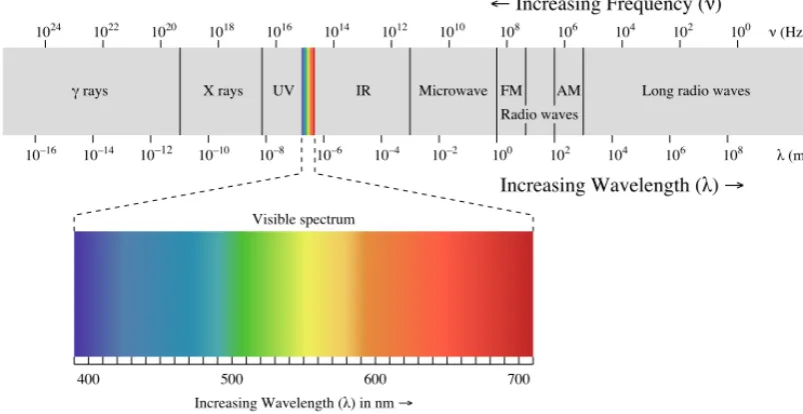
The electromagnetic spectrum is obtained by classifying radiation according to ν and λ (Figure 2.1)
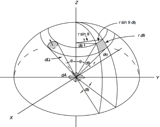
Consider the radiant energy dEλ, in the wavelength interval between λ and λ + dλ, that in the time interval dt crosses an element of area dA, in directions limited to the differential solid angle dΩ, which is oriented to an angle θ with respect to the normal to dA(Figure 2.2). This energy is expressed in terms of the monochromatic intensity, or radiance Iλ:
dEλ =Iλcosθ dA dΩdλ dθ (2.2)
28
Figure 2.1: Spectrum of electromagnetic radiation. From Wikipedia (2015).
Iλ =
dEλ
cosθ dA dΩdλ dθ (2.3) and is measured in W m−3 sr−1.
The monochromatic irradiance is defined as the normal component ofIλ inte-grated over the hemispheric solid angle:
Fλ = Z
Ω
Iλcosθ dΩ (2.4)
In polar coordinates:
Fλ = Z 2π
0
Z π/2
0
Iλ(θ, φ)cosθ sinθ dθ dφ (2.5)
For isotropic radiation:
Fλ =π Iλ (2.6)
29
Figure 2.2: Geometry of radiative transfer in polar coordinates (Liou, 2002)
F = Z ∞
0
Fλ (2.7)
It is measured in W m−2.
2.2
Solar radiation at the top of the atmosphere
The solar constant S is the total solar energy reaching the top of the atmosphere. It is defined as the energy per unit time which crosses a surface of unit area normal to the solar beam at the mean distance between the Sun and the Earth.
The Sun emits an irradiance F of 6.2 × 10⁷ Wm−2. If there is no medium
between the Sun and the Earth, according to the principle of conservation of energy, the energy emitted from the Sun must remain constant at some distance away, thus also in correspondence of the atmosphere of the Earth:
F 4π a2S =S4π r2 (2.8)
30 the solar constant can be expressed as:
S =F aS
r 2
(2.9)
In the ’70 the solar constant was obtained from total solar irradiance measure-ments performed by radiometers aboard many satellites, such as Nimbus 7 Earth Radiation Budget (ERB), Solar Maximum Mission Active Cavity Radiometer Ir-radiance Monitor (SMM ACRIM) 1 and 2, Earth Radiation Budget Experiment (ERBE) aboard the NASA satellites Earth Radiation Budget Satellite (ERBS), NOAA 9 e NOAA 10. From a number of measurements the generally accepted value of 1366 ± 3 Wm−2 has been suggested.
Since the irradiance emitted from the Sun can be considered isotropic, accord-ing to Equation 2.6 the solar intensity is given by I =F/π, thus:
S =I π aS r
2
=IΩ (2.10)
where Ω is the solid angle from which the Earth sees the Sun. If aE is the radius of the Earth, the solar energy intercepted by the Earth is Sπa2
E. If it is uniformly distributed on the surface of the Earth, the solar energy received per unit area per unit time at the top of the atmosphere is:
Q=S
π a2
E 4π a2
E
=S/4≈342W m−2 (2.11)
31
solar radiation fits closely with the blackbody emission at this temperature. How-ever, the ultraviolet (UV) region (< 0.4 µm) of solar radiation deviates greatly from the VIS and IR regions in terms of the equivalent blackbody temperature of the Sun, reaching a minimum of about 4700 K at about 0.14 µm. The energy emitted from the Sun is approximately distributed as follows: 50% in the IR, 40% in the VIS, and 10% in the UV.
Figure 2.3: The 2000 American Society for Testing and Materials (ASTM) E-490 AM0 (air mass 0) Standard Extraterrestrial Spectrum superimposed to the blackbody emission curve at 5782 K
The solar constant is defined for a mean distance between the Earth and the Sun, dm, that is 1.496 × 10¹¹ m, but the actual distribution of solar radiation at the top of the atmosphere depends on the eccentricity of the elliptical orbit of the Earth around the Sun. The point of maximum distance (1.521 ×10¹¹m) is called
aphelion and the Earth is in this position at the beginning of July. The point of minimum distance (1.471 × 10¹¹ m) is called perihelion, and corresponds to the
32 The irradiance on an horizontal surface at the top of the atmosphere also depends on the sun zenith angle:
Fh =F cosθ=S
dm d
2
cosθ (2.12)
whereF is the irradiance on a plane normal to the solar beam, anddis the actual Earth-Sun distance.
2.3
Atmospheric absorption and scattering
Solar radiation entering the Earth’s atmosphere is absorbed and scattered by at-mospheric gases, aerosols, clouds, and the Earth’s surface.
Atmospheric scattering changes the direction of propagation of radiation. It is generally elastic, which means that the scattered radiation has the same frequency as the incident one. However, a small fraction of photons undergoes inelastic scat-tering, in which the energy of radiation is also changed due to electronic transitions in the scattering molecules. This is the so called Raman scattering. Atmospheric scattering can be due to particles of different size, like gas molecules (∼10−4 µm),
33
each particle can scatter the radiation that has been already scattered by other particles. This process is called multiple scattering.
Absorption is the conversion of radiation in another form of energy, like heat. Absorption can be due to atmospheric molecules or aerosols. The UV radiation in the interval 0.2-0.3 µm is mainly absorbed by O3 in the stratosphere. Radiation
with λ shorter than 0.2 µm is absorbed by O2, N2, O and N. In the troposphere,
solar radiation is absorbed in the VIS and IR, mainly by H2O, CO2, O2 and O3.
Figure 2.4 shows the depletion of solar radiation in a cloud and aerosol free atmo-sphere. The top curve represents the solar spectrum at the top of the atmosphere, and the lower curve represents the solar spectrum at sea level. The difference between the two curves gives the combined effects of absorption and scattering of solar radiation by atmospheric gases. In the UV region the depletion of solar energy is dominated by ozone absorption, in the VIS by Rayleigh scattering, and in the near-IR region, which contains about 50% of solar energy, by water vapor absorption.
Scattering and absorption are often associated. Both processes remove energy from incident radiation, and this attenuation is called extinction. In general the amount of energy removed from the original beam of light by a particle is indicated with thecross section. The extinction cross section,σ, is the sum of the absorption and scattering cross sections. When the cross section is associated with a particle dimension, its units are expressed in terms of area (cm2). When it is expressed relative to unit mass, the units are in area per mass (cm2 g−1), and it is called
mass extinction cross section, k. When the cross section is multiplied by the particle number density (cm−3), it is called extinction coefficient, β, and its units
are expressed in terms of length (cm−1).
34
Figure 2.4: Solar irradiance spectrum at the top of the atmosphere and at the surface for a solar zenith angle of 60◦, under clear-sky conditions (Liou, 2002).
angle Θ and the total scattered intensity. P is defined so that its integral over the unit sphere centered on the scattering particle is 4π:
Z 2π
0
P(Θ)sinΘdΘdφ= 4π (2.13)
In terms of scattering cross section, the scattered intensity can be expressed as:
I(Θ) =I0
σs r2
P(Θ)
4π (2.14)
35
2.4
The effect of the Earth’s geometry
Solar radiation interacts with the surface of the Earth at two levels:
1. extraterrestrial irrradiance is influenced by the geometry of the Earth and its revolution and rotation;
2. irradiance at the Earth’s surface is modified by the effects of terrain, includ-ing shadowinclud-ing, elevation, slope and aspect.
The first group of effects depends on the position of the sun above the horizon, which can be calculated by astronomic formulas. Extraterrestrial irradiance falling on a horizontal plane (G0) varies across the year because of the eccentricity of the
Earth’s orbit. Introducing a correction factor, (e), which accounts for the changing distance between the sun and the Earth along the ecliptic, G0 can be expressed
as:
G0 =e Scos(θ) (2.15)
where:
e= 1 + 0.03344cos(j−0.048869) (2.16) The day angle j is expressed in radians:
j = 2π DOY /365.25 (2.17)
and DOY is the day of the year, which varies from 1 on January 1st to 365 (366) on December 31st (?).
36 Here we briefly describe how the direct and diffuse components of irradiance are modified by the Earth’s geometry. The direct component of solar irradiance at the Earth’surface is attenuated, in cloud-free conditions, by atmospheric aerosols and gases. This factors can be accounted for by introducing the Linke turbidity factor, TL:
DIR0 =S e exp(−0.8662TLm δR(m)) (2.18) where m is the relative optical air mass and δR(m) is the Rayleigh optical thickness, both of which can be calculated according the formulation of Kasten (1996).
Direct irradiance on an horizontal surface, DIRh, is calculated as:
DIRh =DIR0sin(h0) (2.19)
whereh0 is the angle between the sun and the horizon (sun elevation).
Direct irradiance on an inclined surface with a solar incidence angle δexp is calculated as:
DIRi =DIR0sin(δexp) (2.20) Shadow casting and surrounding terrain effect can be described by calculating global irradiance as a combination of its direct and diffuse component as follows:
37
2.4.1
Surface albedo
The ground albedo strongly depends on the nature of the surface, and on the spectral and angular distribution of the incoming radiation. The spectral albedo can be expressed as:
α = F ref λ Finc
λ
(2.22)
where Frel
λ is the reflected monochromatic irradiance and Fλinc is the incident one. Broadband albedo can be expressed as:
α = F ref
Finc (2.23)
where Frel is the reflected radiative flux and Finc is the incident one.
Reflected light is generated through two processes: Fresnel reflection and scat-tering. Fresnel reflection describes the process happening between two uniform surfaces with different indexes of refraction. In this case the angle of reflection is equal to the angle of incidence. Diffuse radiation, in contrast, is generated by surface elements whose dimensions are of the same order of magnitude as the wavelengths of incident light. The intensity of the scattered light is only function of the scattering angle, Θ. The distribution of the scattered light is specified in terms of a probability distribution function, which is called phase function and is indicated as P(Θ). P(Θ)sinΘdΘ/2 represents the fraction of scattered radiation which has been scattered through an angle Θ into an incremental ring of solid angle dΩ = 2πsinΘdΘ. The Henyey-Greenstein phase function is an useful formulation
for describing the angular distribution of anisotropic scattering:
P(g,Θ) = 1−g
2
(1 +g2−2g cosΘ)3/2 (2.24)
38
g = 1 2
Z π
0
cosΘP(Θ)sinΘdΘ (2.25)
Forg = 0 the scattering is isotropic, forg <0 most of the radiation is scattered backward, and forg >0 most of the radiation is scattered in the forward direction. If after the first reflection absorption is not so strong, radiation can be scattered multiple times. The effects of single and multiple scattering are described by the empirical formulation of Rahman et al. (1993):
ρ(θ0, θ, φ) =ρ0
cosk−1θ0cosk−1θ
(cosθ0 +cosθ)1−kP(g,Ω) [1 +R(G,∆)] (2.26) where:
G(θ0, θ, φ) = ptan2θ0
+tan2θ− 2tanθ0
tanθ cosφ (2.27)
and
R(G,∆) = 1−ρ0
∆ +G (2.28)
ρ0, k ∆ and g are empirical coefficients specified in Rahman et al. (1993). θ is
Chapter 3
Ground based measurement of
solar irradiance in South Tyrol
3.1
Measurement of radiation components
Ground based measurements allow to monitor solar radiation at point locations accounting for all the geometrical, environmental and atmospheric effects which modify the energy reaching the Earth surface. Regional meteorological services often organize ground based instruments in networks for assessing the spatial dis-tribution of irradiance at regional scale. The usefulness of these networks strongly depends on the spatial density which covers the region of interest, on the quality of the instruments, and on the accuracy of the maintenance procedures.
Direct solar radiation is measured by pyrheliometers, whose receiving surface is normal to the sun beam direction, and whose field of view is limited by an aperture. In order to detect only radiation from the sun and a narrow anulus of sky, WMO recommends that the opening angle is 5◦ and the slope angle is 1◦ (World Meteorological Organization, 2008) (Figure 3.1). To measure continuously, pyrheliometers are equipped with a sun tracker following the sun and allowing a rapid adjustment of the orientation of the instrument.
40
Figure 3.1: View-limiting geometry of a pyrheliometer (Kipp&Zonen, 2008). The opening angle is 2×arctan(R/L) and the slope angle is arctan(R−r)/L.
Global and diffuse radiation are measured by pyranometers (Figure 3.2). The instruments are placed on a plane surface and monitor solar irradiance from a solid angle of 2 π sr, in spectral range from 300 to 3000 nm. When measuring the diffuse component, direct radiation is screened by a shading device. Either a static shadow ring or a sun tracker fitted with a small sphere can be used (Figure 3.3).
41
Figure 3.2: Details of a pyranometer (Kipp&Zonen, 2013).
When the light beam is intercepted, an electronic circuit maintains a constant heat flux from the cavity to the heat sink by adjusting the input power, which can be accurately measured.
Most of the radiation sensors used in meteorological stations make use of a detector which is based on a passive thermal remote sensing element, called ther-mopile. The thermopile warms up responding to the total power absorbed by a black coating, which consists of a non-spectrally selective paint. The coating has many microcavities that trap more than 97% of the incident radiation. The detec-tor, which is made up of a large number of thermocouple junction pairs connected electrically in series, exploits the thermoelectric effect. As the active thermocouple junction (hot junction) absorbs thermal radiation, its temperature increases. The temperature of the other junction (cold junction) is kept constant. The differential temperature between the hot and the cold junction produces an electromotive force directly proportional to the temperature difference. Irradiance can be calculated dividing the output signal by the sensitivity of the instrument:
E ↓= U
42
Figure 3.3: Shading devices for intercepting beam irradiance and measuring diffuse irradiance with a pyranometer (Kipp&Zonen, 2013).
where E ↓ is the irradiance [Wm−2], U is the output of the radiometer [µV]
and S is the sensitivity [µVW−1m2]. The sensitivity of a radiometer, also called
calibration factor, depends on the physical properties of the thermopile, which is unique. Therefore each radiometer has unique calibration factor.
The assessment of the quality of radiation measurement is based on the fol-lowing physical properties of the instrument: sensitivity, stability, response time, cosine response, azimuth response, linearity, temperature response, thermal offset, zero irradiance signal and spectral response (World Meteorological Organization, 2008).
43
The radiometer resolution is the smallest change in radiation which the in-strument can detect. It depends on the physical properties of the detector.
Stability
The non-stability is the percentage change in sensitivity over one year. It is due to deterioration of the black coating by UV radiation.
Cosine and azimuth response
The cosine and azimuth response indicate the dependence of the directional response of the instrument on solar elevation and azimuth. Ideally, the re-sponse of the detector should be proportional to the cosine of the zenith angle of the solar beam, and constant with azimuth angle.
Linearity
The non-linearity of a radiometer is the percentage deviation in the sensitiv-ity over an irradiance range from 0 to 1000 Wm−2compared to the sensitivity
calibration irradiance of 500 Wm−2. The non-linearity effect is due to
con-vective and radiative heat losses at the black absorber surface which make the conditional thermal equilibrium of the radiometer non-linear.
Temperature response
The temperature dependence is the percent deviation with respect to the calibrated sensitivity at +20 ◦C. Some instruments have temperature com-pensation circuits which maintain a constant response over a large range of temperatures.
Thermal offset
The thermal offset is due to heat currents inside the instrument caused by the variation of the instrument temperature according to ambient temperature. It is quantified as the response in Wm−2 to a 5 Kh−1 change in ambient
44
Zero irradiance signal
The zero irradiance signal originates from a temperature difference between the internal components of the instrument. The outer dome is generally colder than the body of the inner absorber. This temperature gradient pro-duces a loss of energy from the absorber, which causes a negative output signal.
Spectral response
The spectral sensitivity is the percentage deviation of the product of spectral absorptance and spectral transmittance from the corresponding mean within the range 300 to 3000 nm.
45
which require that either the zero irradiance signals of all instruments are known, or pairs of identical pyranometers are used in the same configuration. Details on existing calibration methods can be found in World Meteorological Organization (2008).
3.2
The ground network of pyranometers in South
Tyrol
The network of pyranometers installed in the province of Bolzano and managed by the Meteorological Office of the Province is constituted by more than eighty instruments measuring global irradiance. Unfortunately none of them was ever calibrated since the installation, thus the quality of the data is expected to be very low and almost useless for a quantitative assessment. Only few instruments can be used, which were installed during 2009 and collect data without macroscopic measurement error. Figure 3.4 shows the map of these stations, and table 7.1 indicates the name and altitude of the stations included in the map.
Due to the sparse distribution of the measurement stations, the possibility to use this network for an assessment of the spatial distribution of the available so-lar energy in the province is very limited. The topography of the region, in fact, strongly affects irradiance causing an accentuated small scale spatial variability. Consequently, it is not possible to perform an analysis of the spatial correlation between the stations, which would be necessary for applying geostatistical interpo-lation techniques, like kriging. Literature shows, in fact, that the spatial autocor-relation of solar radiation in mountainous terrain does not exceed 1 km (Dubayah, 1992a, 1994; Dubayah and van Katwijk, 1992; Dubayah and Paul, 1995; Oliphant et al., 2003), while the distances between available measurement stations are much longer (Figure 3.5).
46 Wm−2 is typically reached in summer, and a minimum between 20 and 60 Wm−2in
winter, as expected at this latitude. Most of the signals evidence a local minimum in summer, in general in June. This behavior is associated to the secondary peak of convective precipitations which is typically observed in the Alps, and which was particularly intense in summer 2011.
ID NAME ALTITUDE
1 Auer 250
2 Deutschnofen 1470
3 Eyrs - Laas 874
4 Laimburg 224
5 Marienberg 1310
6 Meran Gratsch 330
7 Naturns 541
8 Pfelders 1618
9 Pfinnalm Gsies 2152
10 Plose 2472
11 Sarnthein 970
12 Schlanders 698
13 St. Magdalena in Gsies 1398 14 St. Valentin auf der Haide 1499 15 Stausee Zoggl St. Walburg 1142
16 Sulden 1907
17 Taufers 1235
18 Toblach 1219
47
Figure 3.4: Pyranometers of the province of Bolzano which were installed after 2009.
(a) (b)
(c) (d)
(e) (f)
49
(g) (h)
(i) (j)
(k) (l)
50
(m) (n)
(o) (p)
(q) (r)
Chapter 4
Estimation of diffuse radiation
with decomposition models and
artificial neural networks
4.1
Introduction
In this chapter we compare different kinds of decomposition models which estimate the fraction of diffuse radiation from measurements of global irradiance and other predictor parameters. These models can be used to obtain irradiance direct and diffuse components in regions, such as South Tyrol, whose networks of radiometers only measure global irradiance.
This analysis includes the following models:
1. The polynomial model of Reindl, modified by Helbig et al. (2009);
2. The Boland-Ridley-Laurent logistic model developed by Ridley et al. (2010);
3. A logistic model derived from data collected at three stations in the Alps;
4. A model based on artificial neural networks, developed here from alpine stations data.
52 The first one was chosen among other decomposition models because literature shows that it gives good results in the Eastern Alps (Helbig et al., 2010). The second and the third were selected because they allow to develop a generic logistic function, instead of a piecewise functions, they are easier to implement compared to other methods which exploit more predictors (Skartveit et al., 1998), and they also give better results in the area of interest (Lanini, 2010; Ridley et al., 2010). Finally, the fourth method has never been exploited for estimating irradiance components in the Alps.
4.2
Input data
This analysis is based on hourly averages of data collected at three measurement stations, located in the eastern Alps, where global irradiance and its components are measured. These stations include:
• The BSRN (Baseline Surface Radiation Network) station of Payerne (CH);
• The WRC (World Radiation Centre) station of Davos (CH);
• The EURAC station of Bolzano (IT).
Part of the data was excluded from the analysis, according to the following criteria:
1. Low solar elevation angle, φ, defined as follows:
φ <5◦ (4.1)
This condition is due to the cosine response of pyranometers.
53
F < 5W m−2 (4.2)
F G0
>1.2 (4.3)
Fdif
F >1.1 (4.4)
Fdif G0
>0.8 (4.5)
whereF is global irradiance,Fdif is diffuse irradiance, andG0 is
extraterres-trial irradiance on a horizontal plane.
Two parameters which are used in the decomposition models which are inves-tigated here are the diffuse fraction, defined as follows:
kd= Fdif
F (4.6)
and the clearness index, defined as:
kt = F G0
(4.7)
According to the suggestions of Reindl et al. (1990), two additional conditions were imposed:
kd≥0.9 f or kt<0.2, kd≤0.8 f or kt>0.6.
54
4.3
The model of Reindl
Reindl et al. (1990) developed different decomposition models from data of five sites with at least one year of data for each site. They examined different predic-tor variables which can influence the fraction of diffuse irradiance, and found that kt is the most important under cloudy and partially-cloudy sky conditions, while φ is the most relevant parameter under clear-sky conditions. Consequently, they developed three piecewise correlation models, all of which considered three inter-vals of clearness index, also including ambient temperature and relative humidity. Helbig (2009) combined two of these models, one of which only depends onkt, and the other also depending on φ.
The correlation model is defined as follows:
f or kt ≥0.78 kd= 0.147,
f or0≤kt ≤0.3 kd= 1.020−0.248kt,
f or0.3≤kt ≤0.78 kd= 1.400−1.749kt+ 0.177sin(π/2−θ).
(4.9)
This piecewise correlation generates a discontinuous function, with fixed inter-vals ofkt.
4.3.1
Validation
55
in fact, low values are overestimated and high values are underestimated, while at Davos there is a strong underestimation.
4.4
The model of Boland-Ridley-Laurent (BRL)
The BRL model, presented in Ridley et al. (2010), is a single function which in-cludes more predictors than the Reindl model, but it does not require additional measurements. The added parameters, in fact, can be calculated from measure-ments of global irradiance and from astronomical calculations. Apparent solar time (AST) is included for representing eventual differences in the atmosphere between the morning and the afternoon. The daily clearness index,Kt, is used for describing eventual features typical of the single days:
Kt= P24
j=1Fj
P24 j=1G0j
(4.10)
Finally, a variable called persistence, ψ, is included as a measure of the contin-uance of the global radiation level:
ψ =
kt−1+kt+1
2 sunrise < t < sunset
kt+1 t=sunrise
kt−1 t=sunset
The generic logistic model with five predictors has the following format:
kd=
1
1 +eβ0+β1kt+β2AST+β3φ+β4Kt+β5ψ (4.11) Ridley et al. (2010) estimated the parameters of the model from the data of seven locations worldwide by the minimum least squares method, giving the following expression for the BRL model:
kd =
1
56
(a) (b)
(c) (d)
(e) (f)
57
4.4.1
Validation
Figure 4.2 showskd calculated by equation 4.12 against measured kd. Even if this model seems to cover the spread of the data better than the model of Reindl, the error in the estimation of the hourly average of Fdif is major. This may be due to the fact that the locations used for deriving the model coefficients are too different from the alpine location of interest for this work. For this reason we decided to develop a new logistic model by using data from Bolzano, Davos and Payerne for estimating the parameters. This model is described in the next section.
4.5
The logistic model
We estimated the parametersβ of Equation 4.11 by using hourly averages of global and diffuse irradiance measured at Bolzano from 2011 to 2014, at Davos from 2006 to 2010, and at Payerne from 2000 to 2010.
The logistic function can be expressed as:
Y(X, β) = e β mX
1 +eβ mX (4.13)
where Y represents the diffuse fraction, X the input parameters, and β the coef-ficients of the model.
The log-likelihood function was used as criterion to fit the logistic regression, and its negative was minimized by the Broyden-Fletcher-Goldfarb-Shanno (BFGS) itherative method, by using the BRL coefficients as initial set of parameters:
58
(a) (b)
(c) (d)
(e) (f)
59
Coefficients Bolzano Davos Payerne β0 -1.1488 1.8027 3.1425
β1 -6.9849 -5.9796 -6.5631
β2 0.2571 0.0131 -0.0154
β3 -0.0073 -0.0075 -0.0037
β4 3.2585 3.3625 2.3691
β5 1.1533 0.8778 -0.0864
Table 4.1: Parameter of the logistic function for Bolzano, Davos and Payerne.
4.5.1
Validation
The site-specific logistic models are able to estimate the fraction of diffuse irra-diance with high accuracy, as indicated in Figure 4.3, with MAB of 29 Wm−2 at
Bolzano, 41 Wm−2 at Davos, and 44 Wm−2 at Payerne, and a MBD of 0 Wm−2
at Bolzano, 2 Wm−2 at Davos and 22 Wm−2 at Payerne.
In order to derive a logistic model which is generally applicable at different locations in the Alps, we averaged the coefficients of Table 4.3 and obtained the following expression:
kd = 1
1 +e1.2655−6.5092kt+0.0849AST−0.0062φ+2.9967Kt+0.6482ψ (4.15)
The application of this model gave the results shown in Figure 4.4, which are slightly better than the ones obtained with the site-specific coefficients, with MAB of 38 Wm−2 at Bolzano, 35 Wm−2 at Davos, and 26 Wm−2 at Payerne, and MBD of -4 Wm−2 at Bolzano, -16 Wm−2 at Davos, and 1 Wm−2 at Payerne.
4.6
Artificial Neural Networks (ANN)
60
(a) (b)
(c) (d)
(e) (f)
61
(a) (b)
(c) (d)
(e) (f)
62 estimating diffuse irradiance (Soares et al., 2004; Elminir et al., 2007; Kassem et al., 2009; Kaushika et al., 2014), but no attempt has been made specifically focused on the Alps. This class of algorithms is commonly referred to asmultilayer perceptron, even if it is not composed of perceptrons, but ofsigmoid neurons. Perceptrons, in fact, are neurons connected by weights, which take several inputs and produce a single output which is 0 if the weighted sum of the inputs is below threshold value, and 1 if it is above the threshold. Sigmoid neurons are similar to perceptrons, but their output is modified by anactivation function, so that it is not just 0 or 1, but f(wx+b), where b is calledbias:
b =−threshold (4.16) This characteristic is crucial because it allows the network to learn changing the weights and the bias in order to improve the results.
Such a network of neurons connected by weights allows a nonlinear mapping between an an input and an output vector. The network of nodes generates an output signal, which is modified by a nonlinear activation function. The superposi-tion of many simple nonlinear activasuperposi-tion funcsuperposi-tions allows to approximate complex nonlinear functions. The activation function used here is calledsigmoid function, and is defined by:
σ(z) = 1
1 +e−z (4.17)
where:
z =X j
wjxj−b (4.18)
where xj are the inputs, wj are the weights, and b is the bias.
63
A feed-forward network was used in the work presented here, in which the out-put from one layer is used as inout-put for the next layer, without loops. The gradient descent with momentum back-propagation algorithm was adopted for training the weights of the network.
4.6.1
Method
Two different experiment were performed. The first one only uses data from the station of Payerne, because it offers measurements of a wide set of meteorological parameters. The input features include: global irradiance (F), sun azimuth (α) and zenith (θ) angle, longwave irradiance (LW), aerosol optical thickness (AOT), atmospheric pressure (P), and relative humidity (RH). F, θ, α and AOT were chosen according to well-known physical relationship with the output variable, LW was included as it is closely related to cloud cover, which is a main driver of diffuse radiation, and finally meteorological parameters (T, P, RH) were considered as predictors of the sky conditions.
A feature selection based on the connection weights (Olden et al., 2004) has also been applied for verifying the importance of the predictors.
The second experiment also exploits data from Bolzano and Davos, and is based on different input features, i.e. the same ones used to develop the logistic model in the previous section.
Experiment 1
64
Model Input Parameters 1 F, α, θ, LW 2 F, α, θ, LW, AOD 3 F, α, θ, LW, AOD, P, RH 4 F, α, θ, T, P, RH
Table 4.2: Combinations of input parameters used for training the network.
For each combination of input variables, various network architectures were tested in order to find the optimal one, i.e. the one which produces the small-est error and the biggsmall-est correlation coefficient between small-estimated and measured diffuse irradiance.
Results were compared according to mean absolute bias (MAB) and mean bias deviation (MBD), calculated as in Castelli et al. (2014).
Model Neurons in Hidden Layers R MAB [Wm−2] MBD [Wm−2]
1 50 30 0.860 41 -6
1 40 30 20 10 0.842 45 -9
2 80 40 20 0.880 38 -8
2 100 40 20 0.875 40 -6
2 90 40 20 0.907 33 -7
3 90 40 20 0.870 38 -7
3 60 30 20 0.860 40 -10
4 90 40 20 0.810 50 -6
Table 4.3: Correlation coefficient, MAB and MBD for the network structures which gave the best results.
65
50 Wm−2, and MBD ranges between -6 and -10 Wm−2. The worst model, in terms
of MAB and MBD, is the number 4, which does not include longwave radiation nor AOD.
The observed results are of the same order of magnitude as the ones of the decomposition methods tested in previous sections. However the models developed here have been tested only on a validation dataset extracted from ground-based data which were used for training the network. More validation is required at different sites for testing the exploitation of these models at alpine locations where diffuse irradiance is not measured. The main limitation is the scarcity of high quality data in the region of interest, and the small number of parameters measured by common meteorological stations. One option which will be tested in future is using satellite-based and reanalysis data instead of measured data.
In the following section, another ANN model is developed, exploiting input features which are generally easy to obtain.
Experiment 2
The input variables which are considered in this experiment are: kt, AST, φ, Kt and ψ, as for the logistic model. All the data available at the stations of Bolzano, Davos and Payerne have been aggregated for training the network.
Table 4.4 summarizes the results obtained with different network architectures.
Neurons in Hidden Layers R MAB MBD
90 40 20 0.882 (0.951) 32 (0.077) -17 (-0.044) 120 60 20 0.880 (0.952) 32 (0.076) -19 (-0.048) 80 60 40 20 0.878 (0.950) 34 (0.081) -23 (-0.056) 60 50 40 30 0.826 (0.911) 37 (0.096) -10 (-0.035) 80 40 0.872 (0.953) 34 (0.080) -25 (-0.054)
66
4.7
Validation of logistic and ANN models
The logistic function and the ANN model, developed from the data of Bolzano, Davos and Payerne, have been validated at the station of Weissfluhjoch (CH), at 2540 m.a.s.l.. This procedure allowed to check if these models are enough general to be exploited at different locations in the Alps. Results are summarized in Table 4.5, where MAB and MBD of ANN are the averages with standard deviation of the values obtained for the network architectures included in Table (4.4).
Results are comparable for the two models, but ANN performs slightly better. Both models estimate diffuse irradiance with acceptable accuracy at the considered location, even if its altitude is much different than the one of the stations used for tuning the functions.
Model MAB [Wm−2] MBD [Wm−2]
logistic 51 -17
ANN 43± 1 -10 ± 3
Table 4.5: Validation of the logistic function and of the ANN model at Weiss-fluhjoch.
4.8
Conclusions
In this chapter first we tested two existent decomposition models (the Reindl-Helbig and the BRL) at three alpine stations. Since these models did not give satisfactory results, we developed a site-specific logistic function and an ANN model specifically for the sites of interest.
67
(a) (b)
Figure 4.5: Performances of the logistic model, with coefficients derived from Bolzano, Davos and Payerne, at Weissfluhjoch. The plot on the left hand side shows kd against kt, while the plot on the right hand side shows the scatterplot of modeled diffuse irradiance against measured diffuse irradiance and also include the statistical performances, in terms of MAB, MBD and RMSE, in Wm−2.
Chapter 5
Atmospheric radiative transfer
5.1
The equation of radiative transfer
In Chapter 2 we described qualitatively the processes of solar radiation absorp-tion and scattering taking place in the atmosphere. Here we can formalize them by introducing the equation of radiative transfer (Liou, 2002). When travers-ing a medium of thickness ds, the intensity of a beam of radiation Iλ undergoes weakening due to extinction and strengthening due to emission from the traversed material and multiple scattering from the other directions. The difference between the intensity of the emerging and incoming radiation can be expressed as:
dIλ =−kλρIλds+jλρds (5.1) where ρ is the density of the medium, kλ is the mass extinction cross section for radiation of wavelength λ, and jλ is a source function coefficient. If we define a source function Jλ =jλ/kλ, Equation 5.1 becomes:
dIλ
kλρds =−Iλ+Jλ (5.2)
70 In the wavelength region between 0.2 and 5µm, emissions from the Earth and the atmosphere can be neglected. Supposing that multiple scattering can also be neglected, Equation 5.2 becomes:
dIλ
kλρds =−Iλ (5.3) For a finite thickness s1 of the medium traversed by radiation, Equation 5.3 can
be integrated, giving the emerging intensity:
Iλ(s1) =Iλ(0)exp
−
Z s1 0
kλρds
(5.4)
If the medium is homogeneous, kλ is constant with s, and from Equation 5.4 we obtain the Beer-Bouguer-Lambert law, which describes the decrease in intensity of a beam of radiation traversing an homogeneous absorbing and scattering medium:
Iλ(s1) =Iλ(0)e−kλ
Rs1
0 ρds (5.5)
For many applications concerning radiative transfer in the Earth’s atmosphere, the atmosphere is considered plane-parallel, i.e. atmospheric properties vary only in the vertical direction. In this case it is convenient to substitute the general linear distance s with the distance along the vertical direction, z, thus equation 5.2 becomes:
cosθdIλ(z;θ, φ) kλρdz
=−Iλ