Static and dynamic properties of spin-orbit-coupled Bose-Einstein condensates

Static and dynamic properties

of spin-orbit-coupled

Bose-Einstein condensates

Ph.D. thesis

Supervisor:

Prof. Sandro Stringari

Candidate:

Giovanni Italo Martone

Trento, December 12th, 2014

The preparation for the Ph.D. is always one of the most intense experiences in a person’s life. Here I would like to spend a few words to thank all the people who helped and supported me throughout such a delicate period.

First of all, I would like to acknowledge my supervisor, prof. Sandro Stringari, for his guidance during the last three years. I confess that it is very hard for me to find the proper words to express all my gratitude. I will never forget all the support and the encouragement he has provided me, both from the scientific and the personal point of view, the strong determination with which he helped me each time a new problem appeared, his patience and, above all, his trust in me. I consider having worked with him as one of the greatest privileges I ever had in my life.

I am also grateful to prof. Lev P. Pitaevskii, with whom I had the honor to collaborate during a significant part of my doctoral studies in Trento. I learned a lot from him in every single discussion we had. His kindness, his rigorous scientific mind and his outstanding knowledge of physical problems have represented an important source of inspiration for my research work.

I would like to express my very sincere thanks to Yun Li, the postdoc in the BEC group who followed my first steps as a doctoral student. The support and the friendship of such a pleasant, generous person have helped me a lot in countless difficult situations, even after her departure from Trento. I will never forget my Chinese “little boss”.

I am also indebted towards the permanent members of the experimental team of the BEC Center, Gabriele Ferrari and Giacomo Lamporesi, for patiently providing me much valuable advice on the experimental issues related to the detection of the stripe phase in spin-orbit-coupled Bose gases.

the secretaries, Beatrice Ricci (CNR), Flavia Zanon and Rachele Zanchetta (ERC) and Micaela Paoli (Ph.D. School), and of the technician Giuseppe Froner, who helped me solve all the bureaucratic and technical problems related to my activity at the University of Trento.

Very special thanks are due to my old friend and colleague Leonardo Carcagn`ı, the person who introduced me for the first time into the fascinating world of ultracold gases. His advice of applying for a Ph.D. position in the BEC Center represents one of the most relevant contributions to this thesis work.

Un altro grazie molto speciale vorrei rivolgerlo, con tutto il cuore, alle ragazze dell’open space, Giovanna, Mary e Roberta. A loro assocer`o per sempre uno dei ricordi pi`u belli non solo del mio dottorato, ma di tutta la mia vita. E cos`ı, dopo aver passato tre anni a lamentarmi del nostro ufficio, adesso so che ne sentir`o la mancanza. . .

Non posso non ringraziare il trentino doc Andrea, che mi ha dato un grandissimo sostegno nei momenti pi`u difficili della mia lunga fase di ambientamento a Trento. E non voglio dimenticare i conterranei Daniel, Giuseppe e Matteo, la cui presenza qui `e stata di grande aiuto ad alleviare la nostalgia di casa. Un grazie anche a Fabrizio e Giulio, per la loro amicizia e tutte le stimolanti discussioni che hanno animato i miei rientri a Brindisi.

Introduction 1

1. Theory of standard weakly-interacting Bose gases 5

1.1. Order parameter. Gross-Pitaevskii theory . . . 5

1.1.1. Diluteness criterion . . . 5

1.1.2. Gross-Pitaevskii equation . . . 6

1.2. Dynamic properties of Bose-Einstein condensates . . . 10

1.2.1. Bogoliubov theory and elementary excitations . . . 10

1.2.2. Hydrodynamic formalism and Thomas-Fermi limit . . . 13

1.3. Linear response functions . . . 15

1.3.1. Dynamic structure factor and sum rules . . . 15

1.3.2. Density response function . . . 19

1.3.3. Response function of a weakly-interacting Bose gas . . . 22

2. Ground state of a spin-orbit-coupled Bose-Einstein condensate 25 2.1. Single-particle picture . . . 25

2.2. Many-body ground state . . . 27

2.2.1. Mean-field phase diagram: a variational approach . . . 28

2.2.2. Effects of non-zero detuning and spin-asymmetric interactions . . 33

2.2.3. Experimental results for the ground state . . . 37

2.3. Magnetic polarizability and compressibility . . . 38

2.3.1. Calculation and properties of the magnetic polarizability . . . 38

2.3.2. Thermodynamic compressibility . . . 40

3. Dynamic properties of the uniform phases 41 3.1. Dynamic density response and excitation spectrum . . . 41

3.1.1. Calculation of the dynamic density response function . . . 41

3.1.2. Dynamic density response in the uniform phases . . . 43

3.1.3. Excitation spectrum in the uniform phases . . . 44

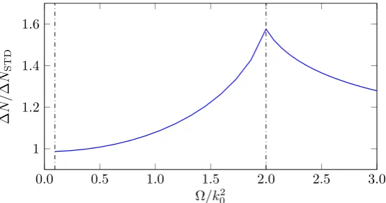
3.1.4. Quantum depletion . . . 46

3.2. Static response function and static structure factor . . . 47

3.3. Velocity and density vs spin nature of the sound mode . . . 49

4. Collective modes in harmonic traps 53 4.1. Dipole mode: a sum-rule approach . . . 53

4.1.1. Sum rules and excitation frequency of the dipole operator . . . 55

4.1.3. Dipole mode and oscillation amplitudes . . . 60

4.2. Hydrodynamic formalism for spin-orbit-coupled Bose gases . . . 61

4.2.1. Hydrodynamic equations and current operator . . . 61

4.2.2. Equilibrium configuration and collective modes . . . 62

5. The stripe phase 67 5.1. Static and dynamic properties of the stripe phase . . . 67

5.1.1. Ground state and excitation spectrum . . . 67

5.1.2. Static structure factor and static response function . . . 70

5.2. Experimental perspectives for the stripe phase . . . 73

Conclusions and outlook 81

A. Coefficients in the density response function 83

Bibliography 85

A large variety of exotic phenomena in solid-state systems can take place when their constituent electrons are coupled to an external gauge field, or in the presence of strong spin-orbit coupling. For example, magnetic fields influencing the motion of the electrons are at the base of the well-known quantum Hall effect [1], whereas spin-orbit coupling, i. e. the coupling between an electron’s spin and its momentum, is crucial for topological insulators [2, 3], Majorana fermions [4], spintronic devices [5], etc.

Ultracold atomic gases are good candidates to investigate these interesting quantum phenomena. Since the first realization of Bose-Einstein condensation in a dilute atomic gas [6, 7, 8], the experimental techniques aiming at creating and manipulating these sys-tems have undergone remarkable improvements. Nowadays one is able to work with both bosonic and fermionic gases, and to realize mixtures of different species [9]. The inter-particle interactions can be tailored practically at will through Feshbach resonances [10]. By using laser light it is possible to achieve a large variety of energy landscapes, including harmonic, periodic, quasiperiodic, and disordered potentials. The dimensionality of the system can also be controlled by using a tight optical confinement of the atomic cloud along one or two directions. This has paved the way to the study of the one-dimensional Tonks-Girardeau gas [11, 12] and the two-dimensional Berezinskii-Kosterlitz-Thouless transition [13].

The main difficulty in employing ultracold gases to simulate condensed-matter phe-nomena like those listed above stems from the fact that atoms are neutral particles, and consequently they cannot be coupled to a gauge field. In addition, they do not exhibit any coupling between their spin and their center-of-mass motion.

In the last few years there have been several proposal to realize artificial gauge fields for quantum gases, thus overcoming the problem of their neutrality [14]. In particular, approaches based on the analogy between the Coriolis and Lorentz forces have been suc-cessfully implemented to realize synthetic gauge fields in rotating neutral fluids, proving to be very efficient for the observation of quantized vortices [15, 16, 17]. An alternative scheme relies on the notion of geometric phase [18], which emerges when the motion of a particle with some internal level structure is slow enough, so that the particle follows adiabatically one of these levels. In such conditions, the particle experiences an effective vector potential. In ultracold atomic gases, several methods to implement these ideas exploit the space-dependent coupling of the atoms with a properly designed configura-tion of laser beams; the synthetic gauge field arises when the system follows adiabatically one of the local eigenstates of the light-atom interaction Hamiltonian (dressed states) [19, 20, 21, 22]. Other approaches are also possible, such as the periodic shaking of an optical lattice with special frequencies, which couples different Bloch bands [23].

coupled to artificial gauge fields [24, 25, 26, 27, 28]. For instance, in the experiment of Ref. [25] a space-dependent atom-light coupling was employed to simulate an effective magnetic field exerting a Lorentz-like force on neutral bosons; this procedure has been used to generate quantized vortices in Bose-Einstein condensates.

Another interesting situation occurs when the local dressed states are degenerate, giving rise to spin-orbit-coupled configurations. In particular, by using a suitable ar-rangement of Raman lasers, the authors of [29] managed to engineer a one-dimensional spin-orbit coupling, characterized by equal Rashba [30] and Dresselhaus [31] strengths, on a neutral atomic BEC. The same scheme has been subsequently extended to realize spin-orbit-coupled Fermi gases [32, 33].

These first experimental achievements have stimulated a growing interest in this field of research, resulting in a wide number of papers devoted to artificial gauge fields and, more specifically, to spin-orbit-coupled quantum gases, both from the theoretical and the experimental side. In this thesis we will focus on the properties of Bose-Einstein con-densates with the kind of spin-orbit coupling first realized by the NIST team [29], which at present is the only one available experimentally. However, it must be pointed out that several other kinds of configurations have been considered theoretically, including pure Rashba and spin-orbit-coupled spin-1 systems. Readers who are interested in a broader overview about spin-orbit-coupled quantum gases and, more generally, about artificial gauge fields on neutral atoms, are referred to some recent reviews [14, 34, 35, 36] and references therein.

Outline. This thesis is organized as follows:

• in Chapter 1 we review some of the main theoretical tools for the investigation of the static and dynamic properties of Bose-Einstein condensed gases. In particular, we first consider the mean-field approach yielding the Gross-Pitaevskii equation, and then we describe the Bogoliubov theory and the hydrodynamic approach for the study of the collective modes. We also give a brief overview on the formalism of linear response functions, which will be widely employed throughout all this thesis;

• in Chapter 2 we illustrate the zero-temperature phase diagram of a spin-orbit-coupled Bose-Einstein condensate. This phase diagram turns out to be very rich, and includes novel quantum phases, such as a spin-polarized plane-wave phase and a stripe phase exhibiting periodic modulations in the density profile. We also study the properties of the various kinds of phase transition that can take place in the system as one varies the spin-orbit and the interaction parameters;

• in Chapter 4 we deal with the collective excitations of the system in the presence of harmonic trapping. A special emphasis is put on the center-of-mass oscillation, whose properties are studied with a sum-rule approach. Its frequency turns out to be deeply affected by the coupling with the spin degree of freedom, and experiences a strong reduction close to the transition between the plane-wave and the single-minimum phases. By resorting to the hydrodynamic formalism we prove that an analogous behavior is shared by all the modes involving a motion of the gas along the direction of the spin-orbit coupling;

• in Chapter 5 we investigate in detail the properties of the stripe phase. Due to the simultaneous presence of superfluidity and crystalline order, this phase shares interesting analogies with supersolids. This is also confirmed by the calculation of the excitation spectrum, which exhibits a double gapless band structure. In the last part of the chapter we present a procedure to enhance the visibility of the fringes and the stability of the striped configurations, thus making the experimental detection of the modulations in the density profile a realistic perspective.

Notations and conventions. In all this thesis, with the exception of Chapter 1, the Planck constant ¯h and the atomic mass m will be set equal to 1.

Vectors will be typeset in bold math characters: r, p, . . . The unit vector along the x direction will be denoted by ˆex.

The subscripts x and _⊥ will be used to denote the components of a vector along the x direction and in the y-z plane, respectively.

When necessary, we will use hats on top of the operators to distinguish them from the numerical quantities: ˆn(r), ˆj(r), . . .

Abbreviations. The following abbreviations will sometimes be used: BEC: Bose-Einstein condensation;

GP: Gross-Pitaevskii;

weakly-interacting Bose gases

The theory of Bose-Einstein condensation has been the subject of a huge literature since much time before its experimental achievement. This chapter is devoted to the presen-tation of some of the main theoretical tools used to study the properties of standard atomic Bose gases. The same tools will be employed in the next chapters to study the physics of spin-orbit-coupled Bose-Einstein condensates. In particular, we review the Gross-Pitaevskii mean-field approach and its conditions of applicability (Section 1.1), and we discuss several methods to investigate the elementary excitations of these sys-tems (Section 1.2). A special emphasis is put on the illustration of the formalism of the linear response theory (Section 1.3). An exhaustive treatment of these concepts is however out of the aims of this thesis; readers interested in more extended discussions can see Refs. [37, 38, 9, 39], on which this chapter is based.

1.1. Order parameter. Gross-Pitaevskii theory

1.1.1. Diluteness criterion

Let us consider an atomic Bose gas of N particles enclosed in a volume V. The position and momentum of each particle will be denoted by rj and pj, respectively, with j ∈

{1,2, . . . , N_} being the particle index. Each couple of atoms interacts through some interatomic potentialV(rj−rk) depending on their relative position. For neutral atoms, any realistic interatomic potential is typically isotropic and short-range. Isotropic means that _V only depends on the relative distance rjk = |rj −rk| of the atoms and not on their orientation in space, while short-range implies that there exists a distance r0, also called the range of the potential, beyond which the interaction is negligible.

In a rarefied atomic gas the mean interparticle distanced= ¯n−1/3, fixed by the average density ¯n=N/V, is much larger than the range of the potential r₀, i.e. the inequality

¯

nr₀3 1 (1.1)

Another consequence of inequality (1.1) is that the distance between two particles is always large enough to allow for the use of the asymptotic expression for the wave function of their relative motion, which is fixed by the scattering amplitude. Therefore all the properties of the system will depend solely on this latter quantity, while the specific details of the two-body potential will not matter. In addition, in the case of a Bose gas at a temperature smaller than the critical temperature for Bose-Einstein condensation, the relevant values of momenta are those satisfying the inequality

pr0 ¯

h 1. (1.2)

At such small values of p the scattering amplitude becomes independent of energy as well as of the scattering angle, and can be safely replaced with its low-energy value. The latter, according to standard scattering theory, is determined by the so-called s-wave scattering length a (see, for example, [38, Sect. 9.2]). In conclusion, one expects that all the effects of the interactions on the physical properties of the gas are determined by one single parameters, which is exactly thes-wave scattering lengtha. In particular, the diluteness condition, which has to be fulfilled in order to apply the theory of dilute gases, can be written as _|a_| n¯−1/3, that is,

¯

n_|a_|3 1. (1.3)

The quantity ¯n_|a_|3 is usually called the gas parameter. Before going on, we notice that, near a Feshbach resonance, the inequality (1.2) is still satisfied, while the diluteness condition (1.3) does not generally hold [38, Sect. 9.2].

1.1.2. Gross-Pitaevskii equation

The many-body Hamiltonian of an atomic Bose gas of N particles can be written as ˆ

H = N X

j=1 _pˆ2

j

2m +Vext(ˆrj)

+ 1 2

N X

j, k=1 j6=k

V(ˆrj−rˆk). (1.4)

where ˆpj =−i¯h∇j denotes the momentum operator of thej-th particle,m is the atomic mass, and we have introduced an external field Vext(ˆr). Let us now rewrite ˆH in the formalism of second quantization, introducing the atomic field operator ˆψ; one has

ˆ H =

Z

drψˆ†(r)

−¯h

2

∇2

2m +Vext(r)

ˆ ψ(r) + 1

2 Z

dr0drψˆ†(r) ˆψ†(r0)V(r0−r) ˆψ(r) ˆψ(r0).

(1.5)

The field operator can be conveniently written in the form ˆ

ψ(r) =X J

where the summation runs over the possible values of a complete set of quantum numbers J, ϕ_J represent a convenient basis of single-particle wave functions, while ˆa_J (ˆa†_J) are the annihilation (creation) operators of a particle in the state ϕJ. The latter obey the bosonic commutation relations

[ˆaJ,ˆa†J0] =δ_JJ0, [ˆa_J,ˆa_J0] = [ˆa† J,ˆa

†

J0] = 0. (1.7)

For example, for a homogeneous system of spinless bosons in a box (Vext = 0), the quantum numbers J can be taken to be the quantized values of the momentum palong the three directions in space, and the corresponding wave functions ϕp would just be plane waves.

Bose-Einstein condensation occurs when one of the single-particle states (hereafter called the condensate, J = 0) is occupied in a macroscopic way, i.e. its occupation number N0 is of the order ofN, while the other single-particle states have a microscopic occupation of order 1. In this case, it is useful to rewrite Eq. (1.6) separating the contribution of the condensate term from the other components:

ˆ

ψ(r) =ϕ0(r) ˆa0+ X

J6=0

ϕJ(r) ˆaJ. (1.8)

The advantage of the representation (1.8) is that it allows to naturally introduce the so-called Bogoliubov approximation, which consists in replacing the operators ˆa0 and ˆ

a†₀ with the c-number √N0. This is equivalent to neglecting the non-commutativity of ˆ

a₀ and ˆa†₀, which is reasonable when dealing with phenomena related to Bose-Einstein condensation, where the occupation number N0 =hˆa†0aˆ0i 1. Indeed, the commutator between ˆa0 and ˆa†0 is equal to 1, while the operators themselves are of the order of

√

N0. Equation (1.8) then becomes

ˆ

ψ(r) =ψ0(r) +δψ(ˆ r), (1.9) where we have defined ψ0 =

√

N0ϕ0 and δψˆ=PJ6=0ϕJaˆJ. In the case of a dilute Bose gas at very low temperatures the noncondensate component δψˆ is negligible, and the system can be described by means of the classical field ψ0 only, which hereafter will be referred to as the condensate wave function or the order parameter. The density n(r) of the gas then corresponds to the condensate density,

n(r) =_|ψ0(r)|2 , (1.10)

and one has the normalization condition R dr_|ψ0(r)_|2 = N0 = N for the condensate wave function ψ0.

The order parameterψ0characterizes the Bose-Einstein condensed phase, and vanishes above the critical temperature needed for the condensation to occur.

number of particles. Its exact meaning can be explained as follows: since the occupation numberN₀ 1, adding one single particle to the condensate does not affect the physical properties of the system. Therefore, a state _|N_i containing N particles is in practice physically equivalent to the states |N + 1i ∝ a†_0|N_i and |N ₋1i ∝ a0|Ni. Thus, it makes sense to writeψ₀ =_hψˆ_i, provided that the states on the left have one less particle in the condensate than the states on the right. This allows to consider the replacement of ˆψ by ψ0 as a kind of mean-field approximation, which is essentially the analogue of the classical limit of quantum electrodynamics, where the classical electromagnetic field entirely replaces the microscopic description in terms of photons.

One should also recall that the field operator ˆψ is defined only up to a constant phase factor. From its definition (1.8), one can see that the order parameterψ0 =

√

N0ϕ0shares the same property. One can always multiply this function by the numerical factor eiα leaving all the physical observables unaffected. Making an explicit choice for the value of the order parameter, and hence for its phase, corresponds to a formal breaking of gauge symmetry. The phase of the order parameter, being related to the superfluid velocity (see Eq. (1.36) below), plays a major role in characterizing the superfluid phenomena (for a more in-depth discussion of the relationship between superfluidity and Bose-Einstein condensation see, for example, [38, Sect. 6.2]).

In order to derive the equation governing the field ψ₀, which can also describe time-dependent configurations, one first has to switch to the Heisenberg picture for the time evolution of a quantum system. In this representation the quantities ˆψ,ψ0 and δψˆhave an explicit time dependence. The quantum field ˆψ(r, t) fulfills the exact equation

i¯h∂

∂tψ(ˆ r, t) = [ ˆψ(r, t),H]ˆ =

−¯h

2

∇2

2m +Vext(r) + Z

dr0ψˆ†(r0, t)V(r0−r) ˆψ(r0, t)

ˆ ψ(r, t).

(1.11)

One could be tempted to say that, in the conditions where the noncondensate component is negligible, we can directly replace ˆψ by ψ0 in the previous equation. However, for a realistic interatomic potential V, such a replacement is not generally correct. Indeed, a realistic potential always contains a short-range term which varies rapidly at distances of the order of r0, thus making quantum correlations important. However, in virtue of the above discussion on the diluteness criteria, we know that the actual form of the two-body potential is not important for describing the macroscopic properties of the gas, the only relevant parameter being the s-wave scattering length. As a consequence, one can replace the bare potential by an effective potential

Veff(r0−r) =g δ(r0−r), (1.12) where the coupling constant g is related to the s-wave scattering length a through [38, Sect. 4.1]

g = 4π¯h 2_a

Hence, we can legitimately make the simultaneous replacement of ˆψ byψ0 and of V by

Veff, and Eq. (1.11) becomes

i¯h∂

∂tψ0(r, t) =

−h¯

2_∇2

2m +Vext(r) +g|ψ0(r, t)| 2

ψ0(r, t). (1.14) Equation (1.14) corresponds to the well-known time-dependent Gross-Pitaevskii equa-tion for the order parameter of the condensate. It was derived independently by Gross [40] and Pitaevskii [41], and is the main theoretical tool for investigating nonuniform dilute Bose gases at low temperatures. The Gross-Pitaevskii equation has the typi-cal form of a mean-field equation, where the order parameter must be typi-calculated in a self-consistent way.

It is worth mentioning that the GP equation (1.14) can also be obtained using a variational procedure. In fact, by imposing the stationarity condition

δ Z

dtdr

−i¯hψ₀∗ ∂ ∂tψ0

+

Z dt E

= 0 (1.15)

to the action, one has the equation

i¯h∂ψ0 ∂t =

δE

δψ∗₀ , (1.16)

for the order parameter, where the energy functional E is given by

E[ψ0] = Z

dr

¯ h2

2m|∇ψ0| 2

+Vext(r)_|ψ0|2+ g 2|ψ0|

4

. (1.17)

The ground state of the system can be easily obtained within the formalism of the Gross-Pitaevskii mean-field theory. For this, one should recall that, for stationary states evolving in time according to the law e−iEt/¯h_{, the relation ψ}

0 =hψˆi yields the law ψ0(r, t) =ψ0(r)e−iµt/¯h (1.18) for the time evolution of the order parameter, with µ= E(N)₋E(N ₋1) _∼ ∂E/∂N being the chemical potential. From (1.14) one finds that ψ0 obeys the so-called time-independent Gross-Pitaevskii equation

−h¯

2_∇2

2m +Vext(r) +g|ψ0(r)| 2

Before concluding the present section, it is useful to briefly discuss some relevant properties of homogeneous systems, where V_ext = 0. In this case the solution of the stationary GP equation (1.19) describing the ground state is independent of r and can be chosen to be real; then one has ψ0(r) =√n, where ¯¯ n =N/V is the average density. This wave function corresponds to a plane-wave state with momentum p = 0. From (1.17) one finds the value

E = gN 2

2V (1.20)

for the ground-state energy. A straightforward calculation yields the results µ=

∂E ∂N

V

=gn ,¯ P =₋

∂E ∂V

N = gn¯

2

2 (1.21)

for the chemical potential1 _{µ and the pressure P. Another useful quantity to calculate} is the thermodynamic compressibility

κ_T =

∂P ∂¯n

−1 = 1

gn¯, (1.22)

which, as expected, tends to infinity in the ideal gas limit g _→ 0. Using the hydrody-namic relation

κT = 1

mc2 (1.23)

for the compressibility one obtains the important result

c= r

g¯n

m (1.24)

for the sound velocity. We will see in Par. 1.2.1 that this result coincides with the value obtained considering the long-wavelength limit of the dispersion relation of the elementary excitations.

The condition of thermodynamic stability implies that the compressibilityκ_T must be positive, i.e. a >0. Hence, we conclude that a dilute uniform Bose-Einstein condensed gas can exist only if the value of thes-wave scattering length is positive. However one can prove that, in the presence of external fields, Bose-Einstein condensed gases can exist, in a metastable configuration, also if the scattering length is negative [38, Chap. 11].

1.2. Dynamic properties of Bose-Einstein condensates

1.2.1. Bogoliubov theory and elementary excitations

Elementary excitations play an important role in the description of the dynamic behavior of a many-body quantum system. In the case of Bose fluids, one of the most relevant

1_{The chemical potential could also be inferred by insertingψ}

0(r) =√n¯into the stationary GP equation

historical examples has been the study of the excitation spectrum of superfluid 4_He. This was the subject of several pioneering works by Landau, Bogoliubov and Feynman (for a more detailed discussion on the dynamic behavior of interacting Bose superfluids see, for example, [42]).

For weakly interacting Bose gases at very low temperatures, Bogoliubov theory rep-resents the main tool for the theoretical investigation of the spectrum of elementary excitations. The starting point of this approach is the time-dependent GP equation (1.14) for the order parameter. We have already seen that the ground state of the sys-tem is characterized by a stationary solution of the form (1.18). In the low-sys-temperature limit, where the elementary excitations do not interact with each other, the excited states can be found by linearizing the GP equation and calculating the corresponding eigenfrequencies ω. This can be done by looking at solutions of the form

ψ0(r, t) = e−iµt/¯hψ0(r) +u(r)e−iωt+v∗(r)eiωt , (1.25) corresponding to small oscillations of the order parameter around the ground-state value. Inserting (1.25) into (1.14), keeping only the terms linear in the complex functionsuand v, and collecting all the terms evolving in time like e−iωt _{and e}iωt_{, one finds the coupled} differential equations

¯

hω u(r) = hHˆ0−µ+ 2g|ψ0(r)|2 i

u(r) +g(ψ0(r))2v(r), (1.26a)

−¯hω v(r) = hHˆ0−µ+ 2g|ψ0(r)|2 i

v(r) +g(ψ₀∗(r))2u(r), (1.26b)

where ˆH0 = −¯h2∇2/(2m) +Vext(r). The solutions of Eqs. (1.26) provide the eigenfre-quencies and the amplitudes u and v of the normal modes of the system.

The formalism we have just discussed was developed by Pitaevskii [41] to investigate the excitations of vortex lines in a uniform Bose gas. It is worth mentioning that this procedure is equivalent to the diagonalization of the Hamiltonian in Bogoliubov approximation, in which one expresses the noncondensate component δψˆ of the field operator (1.9) in terms of quasiparticle annihilation (ˆbJ) and creation (ˆb†J) operators through [43, 44]

δψ(ˆ r, t) = X J6=0 h

uJ(r)ˆbJ(t) +vJ∗(r)ˆb

†

J(t) i

. (1.27)

By imposing the Bose commutation rules to ˆbJ and ˆb†J, one finds that the quasiparticle amplitudes u and v must obey the normalization condition

Z

dr[uJ(r)u∗J0(r)−v_J(r)v_J∗0(r)] = δ_JJ0. (1.28)

Equations (1.26) must in general be solved numerically. However, an analytic solution can be found for uniform gases (Vext = 0), whereµ=gn¯(see Eq. (1.21)) andψ0(r) =

√

Eqs. (1.26) reduce to

¯

hω uq =

¯ h2q2

2m +gn¯

uq+gnv¯ q, (1.29a)

−¯hω vq =

¯ h2q2

2m +gn¯

vq+gnu¯ q. (1.29b)

This eigensystem yields the famous Bogoliubov form [45]

(¯hωB)2 =

¯ h2q2

2m ¯ h2q2

2m + 2gn¯

(1.30)

for the excitation spectrum of a uniform Bose gas. Equation (1.30) coincides with the free-particle energy ¯h2q2/2m at large momenta; at low momenta it instead reduces to the phonon-like dispersion ωB = cq, where the sound velocity c exactly coincides with the value (1.24) given by hydrodynamic theory. The transition between the two regimes takes place when ¯h2q2/2m_∼gn. By setting ¯¯ h2q2/2m =gn¯ with q=ξ−1 one can define the characteristic length ξ = ¯h/√2mg¯n; the physical meaning of ξ will be discussed in Par. 1.2.2.

The oscillation amplitudes relative to the spectrum (1.30), which obey the normaliza-tion condinormaliza-tion |uq|2− |vq|2 = 1 (see Eq. (1.28)), are

uq, vq =±

¯

h2q2/2m+gn¯ 2εB(q) ±

1 2

1/2

, (1.31)

where ε_B(q) = ¯hω_B(q) is given by the positive solution of (1.30).

A relevant quantity that can be evaluated within Bogoliubov theory is the depletion of the condensate due to quantum and thermal fluctuations. For homogeneous system this can be done by introducing theq component

δψˆq = Z

dre−iq·rδψ(ˆ r) =uqˆbq +v∗−qˆb †

−q (1.32)

of the noncondensate term (1.27) of the field operator, which is related to the occupation number nq of particle states with momentum ¯hq6= 0 through the relation

nq =hδψˆq†δψˆqi=|v−q|2+|uq|2hˆb†qˆbqi+|v−q|2hˆb†−qˆb−qi . (1.33) In deriving the previous equation, we made use of the bosonic commutation rules for the operators ˆbq and ˆb†q, as well as of the fact that the averages hˆb−qˆbqi and hˆb†qˆb

Starting from Eq. (1.33), the number of atoms in the condensate at a given temperature T can be calculated through the relation

N0 =N − X

q6=0

nq =N − V (2π)3

Z dq

|vq|2+ |

uq|2+|v−q|2 exp [εB(q)/kBT]−1

. (1.34)

The integral of Eq. (1.34) can be evaluated explicitly at T = 0, yielding the following result for the condensate density:

¯ n0 ≡

N₀ V = ¯n

1− 8

3√π na¯ 31/2

. (1.35)

Hence, the fraction of atoms out of the condensate turns out to be proportional to the square root of the gas parameter ¯na3. This quantity is small because we have assumed that the diluteness condition (1.3) holds. Therefore, result (1.35) represent a justification

a posteriori of the use of the Bogoliubov prescription for the Bose field operators and the perturbative treatment of the noncondensate component at zero temperature.

The measurement of the excitation spectrum of an ultracold atomic gas represents a direct test of the validity of Bogoliubov theory. In particular, in the experiments of Refs. [46, 47, 48] the authors employed two-photon Bragg spectroscopy to probe the excitations in a BEC, and they found a quite good agreement between their data and the theoretical predictions based on the Bogoliubov dispersion law (1.30) (see [49] for a review on the experimental measurement of Bogoliubov excitations in BECs).

1.2.2. Hydrodynamic formalism and Thomas-Fermi limit

Hydrodynamic theory of superfluids provides an elegant and powerful approach to the study of the low-lying collective modes of Bose-Einstein condensed gases. In order to develop the hydrodynamic formalism, one needs to represent the complex order pa-rameter in terms of two real variables, namely its modulus and phase. We then write ψ0(r, t) =pn(r, t) eiφ(r,t)_{, where n represents the superfluid density, while the phase φ} is related to the superfluid velocity vs through the relation [38, Sect. 6.2]

vs = ¯ h

m∇φ . (1.36)

The equations governing the dynamics of n and φ can be obtained by rewriting the stationarity condition of the action (1.15) in terms of these two variables,

δ Z

dtdrhn¯ ∂φ ∂t +

Z dt E

= 0, (1.37)

with the energy functional given by (see Eq. (1.17))

E[n, φ] = Z dr ¯ h2 2m

_∇√n2+ ¯h 2

2mn|∇φ| 2

+V_ext(r)n+g 2n

2

Condition (1.37) yields the continuity equation ∂n

∂t +∇ ·j = 0, (1.39)

where we have defined the current density

j =n¯h

m∇φ , (1.40)

and the equation for the phase ¯

h∂φ ∂t +

¯ h2 2m|∇φ|

2

+Vext+gn− ¯ h2 2m√n∇

2√_n

= 0. (1.41)

When written in terms of the superfluid velocity vs, the second term on the left-hand side of Eq. (1.41) readsmv2

s/2, which does not explicitly depend on the Planck constant ¯

h. The last term on the left-hand side of Eq. (1.41) is instead proportional to ¯h2, and corresponds to the so-called “quantum pressure” term. Its presence is a direct consequence of the Heisenberg uncertainty principle, and reveals that the importance of quantum effects is emphasized in nonuniform gases. However, the quantum pressure can be neglected if the density of the gas changes slowly in space. To make this argument more quantitative, let us indicate by R the typical distance characterizing the density variations taking place in the system. This can be the size of the condensate if we are interested in the ground state, or the wavelength of the density oscillations if we consider time-dependent configurations. Then the quantum pressure term scales as

∇2√_n/√_{n ∼ R}−2_{, and becomes negligible if R is much larger than the characteristic} length

ξ= √ ¯h

2mgn, (1.42)

also called the “healing length” of the condensate (recall that this quantity was already introduced in Par. 1.2.1 to discuss the transition between the phonon and single-particle regimes in the Bogoliubov excitation spectrum). Under such conditions, to which we will refer as the Thomas-Fermi limit, Eq. (1.41) reduces to the simplified form

¯ h∂φ

∂t +

¯ h2 2m|∇φ|

2

+Vext+gn

= 0, (1.43)

which could also be derived from the stationarity condition (1.37) neglecting the quan-tum pressure contribution (first term) in the energy functional (1.38).

Equations (1.39) and (1.43) are the two hydrodynamic equations describing a Bose-Einstein condensed gas in the presence of an external potential Vext. They play an important role in the study of the ground state as well as of the collective modes of such systems.

(1.43) characterized by a time-independent density n =n0(r) and a phase of the form φ =₋µt/¯h, with µthe ground-state chemical potential. From Eq. (1.43) one finds

gn0(r) +Vext(r) = µ . (1.44) Equation (1.44) expresses the condition of local equilibrium for a system whose chemical potential, in the absence of the external field, would be given by the Bogoliubov relation µ = gn. It also allows to estimate the density profile in the presence of an external¯ potential; for example, if Vext is of harmonic type, the predicted density profile has the characteristic shape of an inverted parabola.

The collective modes can be studied in a similar fashion. To this aim, we consider small fluctuations of the density and the phase above the ground-state configuration, i.e. we writen =n0+δnandφ =−µt/¯h+δφ, and we linearize the hydrodynamic equations (1.39) and (1.43). This yields

∂ ∂tδn+

¯ h

m∇ ·(n0∇δφ) = 0, (1.45a)

¯ h∂

∂tδφ+g δn = 0. (1.45b)

By taking the derivative of Eq. (1.45a) with respect totand using Eq. (1.45b), one finds the useful relation

∂2

∂t2δn=∇ ·

c2(r)_∇δn (1.46)

for the density fluctuations of the superfluid, wherec(r) =pgn0(r)/mhas the meaning of a local sound velocity (see Eq. (1.24)).

As we mentioned above, the hydrodynamic theory is expected to correctly describe density oscillations whose wavelength is much larger than the healing length (1.42). In particular, in a uniform system (Vext = 0) the solutions of (1.46) are sound waves propagating with the Bogoliubov velocity (1.24). The main advantage of the hydrody-namic formulation is that it allows to simplify the study of collective oscillations also in trapped configurations, where analytic results for the frequencies of the low-lying discretized modes can be obtained [50, 51, 52].

1.3. Linear response functions

1.3.1. Dynamic structure factor and sum rules

we will focus on density excitations, and we will show how to calculate the response in the case of a weakly-interacting Bose gas. For simplicity, we will focus only on systems at zero temperature; however, the results we are going to show can be extended also to finite temperatures, by including the proper Boltzmann factors in all the formulas [38, Chap. 7].

Let us consider a many-body system described by the Hamiltonian H, and let F and G be two linear operators of physical interest2_{. Without loss of generality one can} take these operator as having vanishing ground-state expectation values. The system is assumed to be coupled to an external field through the time-dependent Hamiltonian

Hpert(t) =−λGe−iωteηt−λ∗G†eiωteηt. (1.47) In Eq. (1.47) λ represents the strength of the external field, which, following the above considerations, will be taken small enough in order to apply linear response theory. The presence of the factor eηt_{, with η positive and small, ensures that att =−∞the system} is governed by the unperturbed HamiltonianH. The adiabatic condition implied by this factor is crucial in order to work in the linear regime.

Let us now calculate the fluctuation δ_hF†_i induced by the presence of the external field. This fluctuation oscillates in time with the same frequency ω as the external perturbation (1.47), and can be written as

δ_hF†_i=λe−iωteηtχ_F†_,G(ω) +λ∗eiωteηtχ_F†_,G†(−ω). (1.48) The quantity χF†,G(ω) is called the “linear response function” or the “dynamic polariz-ability” of the system. It satisfies the propertyχ∗_F†_,G(ω) = χ_F,G†(−ω). As we mentioned before, the response function gives information about the properties of the system in the absence of the external perturbation, and can be straightforwardly calculated using perturbation theory. If the system is in its ground state _|0_i at t= _−∞, then one finds the result [53, 54]

χ_F†_,G(ω) =− 1 ¯ h

X

n

h0|F†_|n_ihn_|G_|0i

ω₋ωn0 + iη −

h0|G_|n_ihn_|F†_|0i

ω+ωn0+ iη

, (1.49)

where _|n_i and ωn0 = (En−E0)/¯h are, respectively, the eigenstates and the excitation frequencies relative to the unperturbed Hamiltonian (H|n_i=En|ni).

A useful quantity is the dynamic structure factor relative to the operator F: SF(ω) =

X

n

|hn_|F_|0_i|2δ(¯hω₋¯hωn0). (1.50)

The quantity|hn_|F_|0i|2 is called the strength of the operatorF relative to the state|n_i. Notice thatS_F vanishes at ω <0, since the excitation energies ¯hω_n0 are always positive.

2 _{Since now on, in this thesis we will omit the “hats” above the symbols for the operators whenever}

In the simplest caseF =G, the response functionχF ≡χF†_,F can be written in terms of the corresponding dynamic structure factor S_F as

χF(ω) =− Z ∞

−∞

dω0

SF(ω0) ω₋ω0_{+ iη} −

SF†(ω0) ω+ω0_{+ iη}

. (1.51)

Using the Dirac relation lim η→0

1

x₋a+ iη = P 1

x₋a −iπδ(x−a), (1.52)

where P is the principal part, the function χ_F can be naturally separated into its real and imaginary parts, which are given by

ReχF(ω) = − Z +∞

−∞

dω0

SF(ω0)P 1

ω₋ω0 −SF†(ω 0

)P 1 ω+ω0

(1.53) and

ImχF(ω) = π(SF(ω)−SF†(−ω)) , (1.54) respectively. Notice that Reχ_F is symmetric with respect toω, while Imχ_F is antisym-metric. Furthermore, for positiveωone finds that ImχF andSF are equal, up to a factor π. The latter property actually holds only at zero temperature, while at finite tempera-ture the two functions can significantly differ; in particular, the dynamic structempera-ture factor exhibits a much stronger dependence on T with respect to ImχF, which consequently represents a more fundamental quantity from the point of view of many-body theory [38, Chap. 7].

In order to determine explicitly the response function or, equivalently, the dynamic structure factor, one generally needs to solve the Schr¨odinger equation and find the eigenstates and the eigenfrequencies of the system. However, one can obtain useful information on the behavior of the dynamic structure factor by resorting to the method of sum rules, which provides an algebraic way to evaluate the moments of the dynamic structure factor

mp(F) = ¯hp+1 Z +∞

−∞

dω ωpSF(ω) = X

n

(En−E0)p|hn|F|0i|2 . (1.55)

A major advantage of this method is that it can reduce the calculation of the dynamical properties of the many-body system to the knowledge of a few key parameters relative to the ground state. Indeed, using the completeness relation P_n|n_ihn_| = 1 and the definition (1.50) for the dynamic structure factor, one easily obtains the following sum rules:

where the average is taken on the ground state, and we have considered only the lowest moments. In general, S_{F 6}=S_F† so that the sum rules (1.57) and (1.59) may also differ from zero. The sum rules (1.57) and (1.58) are related to the high-frequency expansion of the dynamic response function (1.51), which is given by

χF(ω)ω→∞ =−

1 ¯ hωh[F

†

, F]i − 1

(¯hω)2h[F

†

,[H, F]]i. (1.60) Notice that the leading term in the expansion, which behaves like 1/ω, vanishes if F commutes with its adjoint, as in the case of the density operator (see next paragraph). Another interesting property is that the sum rules (1.56) and (1.59) containing the anticommutators do not enter the above expansion. In the opposite limit of smallω, the dynamic polarizability approaches its static limit (static polarizability) according to the law

χF(0) ≡χF(ω)ω→0 =m−1(F) +m−1(F†), (1.61)

where m−1 is the inverse energy-weighted moment of the dynamic structure factor. In contrast to the moments with p _≥ 0, the inverse energy-weighted moments cannot be reduced in terms of commutators, and they are usually evaluated through the direct calculation of the static response.

One of the advantages of the formalism of linear response function is that, in the T = 0 limit we are considering, where the dynamic structure factor vanishes for ω <0, it allows to derive rigorous upper bounds for the energy ¯hωmin of the lowest state excited by the operator F. In particular, for any value of p, the following inequalities hold:

¯

hωmin ≤

mp+1(F) mp(F)

(1.62)

and

¯

hωmin ≤ s

mp+1(F) mp−1(F)

. (1.63)

Analogously, one can prove that the moments of F satisfy mp+1(F)

mp(F) ≥

mp(F) mp−1(F)

, (1.64)

which for p= 0 provides an upper bound to the non-energy-weighted moment m0: m0(F)_≤pm1(F)m−1(F). (1.65)

1.3.2. Density response function

In this paragraph we will apply the formalism of linear response theory to the most important problem of the density response function.

Let us consider the q component

ˆ ρq =

N X

j=1

e−iq·rj ₌

Z

dre−iq·rn(ˆ r) (1.66)

of the density operator

ˆ n(r) =

N X

j=1

δ(r₋rj), (1.67)

where rj is the coordinate operator of the jth particle. The density response function, hereafter called χ(q, ω), is obtained by making the choice F = G = δρˆ†_q, with δρˆ†_q =

ˆ

ρ†_{q− h}ρˆ†_qi, in Eq. (1.49). Notice that the ground-state expectation value hρˆ†_qivanishes in uniform systems if q₆= 0. One can write

χ(q, ω) =−1

¯ h

X

n "

h0|δρˆq|ni 2 ω₋ωn0+ iη −

_h0_|δρˆ†_q|n_i2 ω+ωn0+ iη

#

. (1.68)

Analogously, the dynamic structure factor takes the form (see Eq. (1.50) with F =δρˆ†_q) S(q, ω) =X

n

_h0|δρˆq|ni 2

δ(¯hω₋¯hωn0). (1.69) The relevance of the dynamic structure factor resides in the fact that it characterizes the scattering cross-section of inelastic reactions where the scattering probe transfers mo-mentum ¯hqand energy ¯hω to the system, as happens, for example, in neutron scattering from liquid helium.

Let us now discuss the behavior of the moments mp(q) = ¯hp+1

Z +∞

−∞

dω ωpS(q, ω) (1.70)

of the dynamic structure factor. In many cases these can be evaluated explicitly through the method of sum rules. The derivation of sum rules for the density operator can be greatly simplified if the unperturbed configuration is invariant with respect to either parity or time reversal, in which case the following identity holds:

S(q, ω) =S(₋q, ω). (1.71)

The non-energy-weighted (p= 0) moment can be expressed as

m0(q) = ¯h Z +∞

−∞

dω S(q, ω) =N S(q), (1.72) where the quantity

S(q) = 1

N hρˆqρˆ−qi − |hρˆqi| 2

(1.73) is the so-called static structure factor, which is determined by the fluctuations of the density. Equation (1.73) was derived using Eq. (1.69) and the completeness relation P

n|nihn| = 1. At small q the static structure factor is sensitive to dynamical cor-relations. However, at high q only incoherent processes are important, and the sum ˆ

ρ†_qρˆq = P

j,kexp [iq·(rj −rk)] is exhausted by the j = k term; as a consequence, one finds the model-independent asymptotic behaviorS(q)q→∞ = 1. It is worth pointing out

that the static structure factor is always symmetric under inversion ofq into ₋q, even in the cases where the identity (1.71) does not hold; this general feature follows from the expression (1.73) and the commutation relation involving the density operators:

S(q)−S(−q) = 1

Nh[ˆρq,ρˆ−q]i= 0. (1.74) Another very relevant sum rule is given by the energy-weighted moment

m1(q) = ¯h2 Z +∞

−∞

dω ω S(q, ω) = 1 2h[δρˆ

†

q,[H, δˆρq]]i, (1.75) where we have used the completeness relation and the identity (1.71). To calculate the double commutator of Eq. (1.75), we first notice that, for velocity-independent po-tentials, only the kinetic energy contributes to the inner commutator [H, δρˆq], which becomes

[H, δρˆq] =−¯hq·ˆjq, (1.76) where

ˆ

jq = 1 2m

N X

j=1

pje−iq·rj+ e−iq·rjpj

= Z

dre−iq·rˆj(r) (1.77) is the q component of the current density operator

ˆ

j(r) = 1 2m

N X

j=1

[pjδ(r−rj) +δ(r−rj)pj] . (1.78)

The double commutator can now be evaluated explicitly, yielding [δρˆq,[H, δρˆ−q]] = N¯h2q2/m. Then, one finds the model-independent result

m1(q) = ¯h2 Z +∞

−∞

dω ω S(q, ω) = Nh¯ 2_q2

also known as the f-sum rule [55, 56]. This is the analogue of the well-known dipole Thomas-Reich-Kuhn sum rule for atomic spectra, and represents a remarkable result in many respects. First, it holds for a wide class of many-body systems, independent of statistics and temperature. Second, as we shall see later, it can be used, together with other moments, to estimate the frequency of the collective excitations. In addition, the f-sum rule is also deeply connected to the equation of continuity. This can be seen by taking the inverse Fourier transform of Eq. (1.76) and switching to the Heisenberg representation, which yields

∂

∂tˆn(r, t) +∇ ·jˆ(r, t) = 0. (1.80) By taking the average of the previous equation over an arbitrary configuration out of equilibrium, one recovers the usual conservation law of the particle number.

The double commutator appearing in Eq. (1.75) also fixes the high-ω behavior of the dynamic response function (recall that the term 1/ω identically vanishes in this case):

χ(q, ω)ω→∞ =−

1

(¯hω)2h[δρˆq,[H, δρˆ−q]]i=− N q2

mω2 . (1.81)

Hence, for systems where the inversion property (1.71) holds, one finds the relation χ(q, ω)ω→∞ = −2m1(q)/(¯hω)2 between the density response function and the

energy-weighted moment of δρˆq. However, the validity of Eq. (1.81) is not restricted to this hypothesis.

Finally, let us consider the inverse energy-weighted moment

m−1(q) = Z +∞

−∞

dωS(q, ω)

ω . (1.82)

From Eq. (1.61) one finds that this moment is related to the static response of the system,

N χ(q)_≡χ(q,0) = 2m−1(q), (1.83)

where we have again made use of Eq. (1.71). In uniform systems the low-q limit of the static response can be related to the thermodynamic compressibility κ_T. In fact, in this case the deformations induced by the external force can be exactly expressed in terms of the local changes of the pressure, and a simple calculation gives the results

lim q→0

Z +∞

−∞

dωS(q, ω)

ω =

N κT

2 =

N

2mc2 , (1.84)

where we made use of Eq. (1.23) relating the compressibility to the sound velocity c. Equation (1.84) is known as the compressibility sum rule.

for the energy of the elementary excitations in terms of the static structure factor, which corresponds to the so-called Feynman energy [57]

¯

hωF(q) =

m1(q) m0(q) =

¯ h2q2

2mS(q), (1.85)

where we have used the sum rules (1.72) and (1.79). The Feynman estimate has been extensively used to discuss the excitation spectrum of superfluid helium as a function of

q. Inequality (1.65), in combination with the f-sum rule (1.79) and the relation (1.61), instead connects the static structure factor to the static response function:

S(q)≤

s ¯ h2q2

4m χ(q). (1.86)

In the small-q limit, where χ(q) approaches the compressibility κT = 1/mc2, one finds the useful result that the static structure factor vanishes linearly asq _→0,

S(q)_≤ ¯hq

2mc. (1.87)

Still in the same limit, using Eq. (1.63), one finds that the lowest excitation frequency vanishes like

ωmin(q)≤cq . (1.88)

The above results have been derive on a very general basis. No assumption on the exact nature of the system has been made, except for the validity of the f-sum rule and the fact that the compressibility is finite. With this simple assumptions, we proved that the excitation spectrum is gapless (Eq. (1.88)) and that the density fluctuations, given by S(q), are vanishingly small in the long-wavelength limit (Eq. (1.87)). In the next paragraph we will prove that, in the special case of a standard weakly-interacting Bose gas, the bounds (1.87) and (1.88) become identities, since all the moments are exhausted by a single excited state. Actually, in the dilute Bose gas this is true for all values of

q. It is also remarkable that in superfluid helium, a system characterized by strong correlations, the bounds (1.87) and (1.88) become identities in the small-q limit.

1.3.3. Response function of a weakly-interacting Bose gas

In this paragraph we present a method to calculate the density response function of a weakly-interacting Bose gas. This approach is based on the formalism of the Bogoliubov theory, which has already been exploited in Par. 1.2.1 to find the excitation spectrum of this system. An equivalent procedure, which relies on the formalism of quasiparticle operators, is illustrated in [38, Sect. 7.6].

equation (1.14) with an additional term accounting for the presence of the perturbation, i¯h∂

∂tψλ(r, t) =

H0+Vλ(r, t) +g|ψλ(r, t)|2

ψλ(r, t), (1.89) with H0 = −¯h2∇2/2m+Vext(r) and Vλ(r, t) = −λei(q·r−ωt)eηt + H.c. To simplify the notation, in the next steps of the calculation we will omit the small imaginary part η of the oscillation frequency; it will be restored at the end, once the full expression of the density response function will be available.

In the limit of smallλ one can look for solutions of Eq. (1.89) corresponding to small-amplitude oscillations around the unperturbed ground-state configuration, namely

ψλ(r, t) = e−iµt/¯hψ0(r) +uλ(r)e−iωt+v∗λ(r)eiωt

. (1.90)

This ansatz is formally equal to the one of Eq. (1.25), but now the small amplitudes uλ and vλ are proportional to the perturbation strength λ, and depend on both its wave vector q and frequency ω. In order to calculate these amplitudes, one must insert Eq. (1.90) into (1.89), keep only the linear terms in λ,uλ and vλ, and collect separately the terms evolving in time like eiωt_{and e}−iωt_{. This procedure yields the following coupled} differential equations:

h ˆ

H0−µ+ 2g|ψ0(r)|2−¯hω i

uλ(r) +g(ψ0(r))2vλ(r) = λeiq·r, (1.91a) h

ˆ

H0−µ+ 2g|ψ0(r)|2+ ¯hω i

vλ(r) +g(ψ0∗(r)) 2

uλ(r) =λeiq·r_{. (1.91b)} Once the previous equations have been solved, it is straightforward to calculate, up to linear order in λ, the fluctuation of the density

δnλ(r, t) =|ψλ(r, t)|2_{− |ψ0(r)|}2 _{= [ψ}∗

0(r)uλ(r) +ψ0(r)vλ(r)] e

−iωt_{+ c.c. (1.92)} The q component of δnλ is then found to exhibit the typical structure, already shown in Eq. (1.48), for the fluctuation of an operator caused by an external perturbation,

δρq,λ(t) = Z

dre−iq·r_{δnλ(r, t) = λχ(q, ω)e}−iωt_+λ∗

˜

χ(q,₋ω)eiωt, (1.93) where the density response function, corresponding to the coefficient of the term oscil-lating in time like e−iωt_{, is given by}

χ(q, ω) = λ−1 Z

dre−iq·r_[ψ∗

form uλ(r) = uλeiq·r _{and v}

λ(r) = vλeiq·r, with uλ and vλ satisfying the inhomogeneous equations

¯ h2q2

2m +gn¯−¯hω

uλ+gnv¯ λ =λ , (1.95a)

¯ h2q2

2m +gn¯+ ¯hω

v_λ+gnu¯ _λ =λ , (1.95b) where we have used the results ψ0(r) = √¯n and µ = g¯n for the uniform Bose gas. Solving Eqs. (1.95) one finds that the amplitudes are given by

u_λ, v_λ =_∓1 ¯ h

ω_±hq¯ 2/2m ω2_−ω2

B(q)

√

¯

n λ , (1.96)

where ωB(q) is the Bogoliubov dispersion law (1.30). After inserting these results into Eq. (1.94) and carrying out the integration over r, we finally obtain the expression of the density response function for a weakly-interacting Bose gas,

χ(q, ω) =₋

1

ω₋ωB(q) + iη −

1

ω+ωB(q) + iη

Nh¯2q2

2mεB(q), (1.97) whereε_B = ¯hω_B, and we have restored the small imaginary part of the frequency by re-placingωwithω+iηclose to the poles. Comparing Eq. (1.97) with the general structure of the density response function given in Eq. (1.68), one finds that in weakly-interacting Bose gases only a single state is excited by a density perturbation, its frequency being given by the Bogoliubov expression (1.30).

The dynamic structure factor can be easily obtained by applying the Dirac relation (1.52) to the response function (1.97) and taking its imaginary part. One finds

S(q, ω) = π−1Imχ(q, ω) =N ¯h 2

q2

2mεB(q)δ(¯hω−εB(q)) (1.98) for ω_≥0, while S(q, ω) = 0 for ω <0. Using this expression for the dynamic structure factor, one can immediately see that the f-sum rule (1.79) is satisfied, while the inverse energy-weighted moment reads

m−1(q) =N ¯ h2q2 2mε2

B(q)

. (1.99)

In the small-q limit one has ε_B(q) = ¯hcq, and therefore Eq. (1.99) approaches the con-stant value N/2mc2_{, in agreement with the general result (1.84) for the compressibility} sum rule.

The static structure factor is also easily evaluated and takes the nontrivial form S(q) = ¯h

2_q2

2mεB(q). (1.100)

Bose-Einstein condensate

A key feature of spin-orbit-coupled Bose-Einstein condensates is their rich phase dia-gram. The aim of this chapter is to illustrate some relevant ground-state properties of the quantum phases exhibited by these systems. We first discuss the situation at the single-particle level (Section 2.1), showing how the spin-orbit Hamiltonian is realized experimentally, and highlighting the peculiar features of the single-particle energy spec-trum. Then we consider the many-body ground state (Section 2.2), whose properties are investigated within the mean-field Gross-Pitaevskii theory through a variational ap-proach. We point out the occurrence of novel configurations, including a striped and a spin-polarized phase, and we study the properties of the various phase transitions that can take place in the system. Finally, we calculate two important quantities character-izing the system in all its quantum phases, namely the magnetic polarizability and the compressibility (Section 2.3). This chapter is based on Refs. [58, 59, 60].

2.1. Single-particle picture

The experimental setup employed in Ref. [29] to realize spin-orbit coupling consists of a 87_{Rb Bose-Einstein condensate in the F = 1 hyperfine manifold, with a bias magnetic} field providing a nonlinear Zeeman splitting between the three levels of the manifold. The BEC is coupled to the field of two Raman lasers having orthogonal linear polariza-tions, frequencies ωL and ωL+ ∆ωL, and wave vector difference k0 =k0eˆx, with ˆex the unit vector along the x direction. The laser field induces transitions between the three states characterized by a Rabi frequency Ω fixed by the intensity of the lasers. This Raman process is illustrated schematically in Fig. 2.1. The frequency splitting ωZ be-tween the states_|F = 1, mF = 0iand|F = 1, mF =−1iis chosen to be very close to the frequency difference ∆ωL between the two lasers, while the separationωZ−ωq between

|F = 1, mF = 0i and |F = 1, mF = +1i contains a large additional shift from Raman resonance due to the quadratic Zeeman effect. This implies that the state _|mF = +1i can be neglected, and we are left with an effective spin-1/2 system, with the two spin states given by _|↑i = _|mF = 0i and |↓i = |mF =−1i. The single-particle Hamiltonian of this system takes the form (we set ¯h =m = 1)

h₀ = p 2 2 +

Ω

2σxcos(2k0x−∆ωLt) + Ω

2σysin(2k0x−∆ωLt)− ωZ

|−1_i=_|↓i

|0i=|↑i

|+1_i

δ/2

δ/2

ωq+ 3δ/2

ωZ

BEC

Figure 2.1. Level diagram. Two Raman lasers with orthogonal linear polarizations couple the

two states|↑i=|mF = 0iand|↓i=|mF =−1iof theF = 1 hyperfine manifold of87Rb, which

differ in energy by a Zeeman splittingωZ. The lasers have frequency difference ∆ωL=ωZ+δ,

whereδ is a small detuning from the Raman resonance. The state_|mF = +1ican be neglected

since it has a much larger detuning, due to the quadratic Zeeman shiftωq.

respect to helicoidal translations of the form eid(px−k0σz)_{, consisting of a combination of}

a rigid translation by distance d and a spin rotation by angle ₋dk0 around thez axis. Let us now apply the unitary transformation eiΘσz/2_{, corresponding to a position and}

time-dependent rotation in spin space by the angle Θ = 2k0x −∆ωLt, to the wave function obeying the Schr¨odinger equation. As a consequence of the transformation, the single-particle Hamiltonian (2.1) is transformed into the translationally invariant and time-independent form

hSO₀ = 1 2

(px−k0σz)2+p2⊥

+Ω 2σx+

δ

2σz. (2.2)

The spin-orbit nature acquired by the Hamiltonian results from the noncommutation of the kinetic energy and the position-dependent rotation, while the renormalization of the effective magnetic fieldδ= ∆ωL−ωZ results from the additional time dependence exhib-ited by the wave function in the rotating frame. The new Hamiltonian is characterized by equal contributions of Rashba [30] and Dresselhaus [31] couplings. It has the peculiar property of violating both parity and time-reversal symmetry. It is worth pointing out that the operator p entering (2.2) is the canonical momentum −i∇, with the physical velocity being given byv± =p∓k0eˆx for the spin-up and spin-down particles. In terms of pthe eigenvalues of (2.2) are given by

ε±(p) =

p2_x+p2_⊥

2 +Er± s

k0px− δ 2

2 + Ω

2

4 (2.3)

−2 −1 0 1 2

−0.5 0 0.5 1

|↑i |↓i |↓i

|↑i

px/k0 ε±

(

px

)

/k

2 0

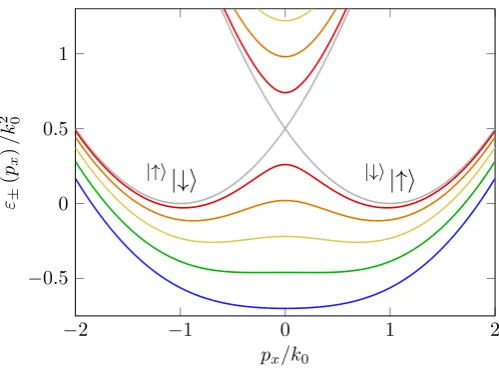
Figure 2.2. Single-particle dispersion (2.3) atδ = 0. Eigenergies calculated for Raman coupling

ranging from Ω = 0 (grey) to Ω = 2.4k2₀ (blue). The two minima in the lower branch disappear

at Ω = 2k2₀.

We now focus on the case δ = 0 and Ω ≥ 0. In Fig. 2.2 we plot the dispersion (2.3) as a function of px, for different values of Ω. The lower branch ε−(p) exhibits, for

Ω < 2k2

0, two degenerate minima at momenta p = ±k0 p

1−Ω2_/4k4

0eˆx, both capable to host Bose-Einstein condensation. At larger values of Ω the spectrum has instead a single minimum at p = 0. The effective mass of particles moving along x, fixed by the relation m/m∗ = d2_ε/dp2

x, also shows a nontrivial Ω dependence. Near the minimum one finds [61]

m m∗ =

        

1₋

Ω 2k2

0 2

for Ω <2k2 0

1− 2k

2 0

Ω for Ω >2k 2 0

(2.4)

Thus, the effective mass exhibits a divergent behavior at Ω = 2k2

0, where the double-well structure disappears and the spectrum has a p4_x dispersion near the minimum.

Before concluding the present section, it is worth mentioning that a single-particle dispersion similar to (2.3) can also be achieved by trapping the atoms in a shaken optical lattice, as has been recently realized experimentally [28]. In such systems, different Bloch bands coupled through lattice shaking bear several analogies with the spin states involved in the Raman process described above [62].

2.2. Many-body ground state

the many-body Hamiltonian takes the form

H =X

j

hSO₀ (j) + 1 2

X

σ, σ0 Z

drg_σσ0nˆ_σ(r)ˆn_σ0(r), (2.5)

where hSO₀ is given by (2.2), j = 1, . . . , N is the particle index, and σ, σ0 are the spin indices (_↑,_↓=_±) characterizing the two spin states. The spin-up and spin-down density operators entering (2.5) are defined by ˆn±(r) = P_jP±,jδ(r−rj), whereP± = (1±σz)/2

denotes the two spin projection operators. The relevant coupling constantsgσσ0 = 4πa_σσ0 in the different spin channels are fixed by the corresponding s-wave scattering lengths aσσ0. Notice that the two-body interaction terms are not affected by the spin rotation discussed in Sect. 2.1.

2.2.1. Mean-field phase diagram: a variational approach

To investigate the ground state of the system we resort to the Gross-Pitaevskii mean-field approach, which has been discussed in Sect. 1.1. For this, we introduce the two-component wave function Ψ = (ψ↑ ψ↓)T describing our spin-1/2 condensate, and we

write the energy functional associated to Hamiltonian (2.5) as

E[Ψ] = Z

dr

"

Ψ†hSO₀ Ψ + 1 2

X

σ, σ0

gσσ0 Ψ†P_σΨ Ψ†P_σ0Ψ #

. (2.6)

When written in terms of ψ↑,↓, Eq. (2.6) reads

E[ψ↑, ψ↓] = Z

dr

" ψ∗↑(r)

(px−k0)2+p2⊥

2 ψ↑(r) +ψ

∗ ↓(r)

(px+k0)2+p2⊥

2 ψ↓(r) # + Z dr Ω 2

ψ_↑∗(r)ψ↓(r) +ψ∗↓(r)ψ↑(r)

+δ 2

|ψ↑(r)|2 − |ψ↓(r)|2

+ Z

drhg↑↑

2 |ψ↑(r)| 4

+g↓↓

2 |ψ↓(r)| 4

+g↑↓|ψ↑(r)|2|ψ↓(r)|2 i

. (2.7)

The use of the mean-field description for a spin-orbit-coupled Bose gas can be justifieda posterioriby estimating the quantum depletion of the system and proving that it remains small for reasonable values of the spin-orbit coupling parameters; this calculation is postponed to Sect. 3.1.

Since now on, in this thesis we will assume δ = 0 and equal intraspecies interactions g↑↑ = g↓↓ ≡ g, unless otherwise specified; the effects of the presence of a non-vanishing

magnetic detuning and of spin-asymmetric interactions on the ground state will be briefly discussed in Par. 2.2.2.

The Gross-Pitaevskii equation for the spinor order parameter can be deduced in the same way as in Sect. 1.1 and reads

i∂Ψ ∂t =

hSO₀ + +1

2(g+g↑↓) Ψ

†

Ψ+1

2(g−g↑↓) Ψ

†

σ_zΨσ_z

where the right-hand side corresponds to the functional derivative δE[Ψ]/δΨ† _{of the}

energy (2.6).

The ground-state wave function in uniform matter can in principle be determined by looking for a stationary solution of Eq. (2.8) of the form Ψ(r, t) = e−iµt_{Ψ(r). However,} here we will use a different approach, consisting in a variational procedure based on the following ansatz [58]:

Ψ (r) = √¯n

C+

cosθ

−sinθ

eik1x_+C −

sinθ

−cosθ

e−ik1x

, (2.9)

where ¯n = N/V is the average density, and k1 represents the canonical momentum where Bose-Einstein condensation takes place. For a given value of ¯n, k0, Ω and of the coupling constants g and g↑↓, the variational parameters are C+, C−, k1 and θ. Their values are determined by minimizing the energy (2.7) with the normalization constraint R

drΨ†_{Ψ =N, i. e. |C}

+|2+|C−|2 = 1. Minimization with respect toθyields the general

relation

θ = 1

2arccos k₁ k0

(0≤θ_≤π/4) (2.10)

fixed by the single-particle Hamiltonian (2.2). Once the other variational parameters are determined, it is possible to calculate key physical quantities like, for example, the momentum distribution accounted for by the parameter k1, the total density

n(r) = Ψ†Ψ = ¯n "

1 + 2|C+C−| p

k₀2₋k2₁ k0

cos (2k1x+φ) #

, (2.11)

the longitudinal (sz(r)) and transverse (sx(r), sy(r)) spin densities sz(r) = Ψ†σzΨ = ¯n _|C+|2− |C−|2

k1 k0

, (2.12)

sx(r) = Ψ†σxΨ =−n¯ "p

k2 0−k12 k0

+ 2|C+C−|cos (2k1x+φ) #

, (2.13)

sy(r) = Ψ†σyΨ = ¯n|C+C−|

2k1 k0

sin (2k1x+φ) , (2.14)

with φ the relative phase betweenC₊ and C−, and the corresponding spin polarizations

hσki= R

drsk(r)/N withk=x, y, z. Before going on, we notice that results (2.13) and (2.14) hold in the spin-rotated frame where the Hamiltonian takes the form (2.5). Since the operators σ_x and σ_y do not commute with σ_z, the transverse spin density along x calculated in the original laboratory frame exhibits an additional oscillatory behavior sx(r) cos (2k0x−∆ωLt)−sy(r) sin (2k0x−∆ωLt), with sx(r) andsy(r) given by (2.13) and (2.14), characterizing the laser potential of Eq. (2.1) (an analogous result holds for the transverse spin density along y).

values of the canonical momentum k1. In this case the energy is independent of C±,

reflecting the degeneracy of the ground state.

The same ansatz is well suited also for discussing the role of interactions, which cru-cially affect the explicit values ofC+, C− and k1. By inserting (2.9) into (2.7), one finds

that the energy per particleε =E/N takes the form ε= k

2 0 2 −

Ω 2k0

q

k2₀₋k₁2₋F(β) k 2 1 2k2

0

+G1(1 + 2β) , (2.15) where we have defined the dimensionless parameter β=|C+|2|C−|2 ∈[0, 1/4] and the

function

F(β) = k₀2₋2G2

+ 4 (G1+ 2G2)β , (2.16)

with the interaction parametersG1 = ¯n(g+g↑↓)/4 andG2 = ¯n(g−g↑↓)/4 (here we assume

G₁ > 0 to ensure the stability of the system in the absence of external potentials