Remote Control of Space Robots Change-Adaptive in its
External Environment
https://doi.org/10.3991/ijoe.v15i07.10219
Feliks Kulakov
St. Petersburg Institute of Informatics and Automation of the Russian Academy of Sciences (SPIIRAN), Saint Petersburg, Russia
Seifedine Kadry (*)
Beirut Arab University, Beirut, Lebanon [email protected] Gennady Alferov, Polina Efimova
Saint Petersburg State University, Saint Petersburg, Russia
Abstract—In the paper a method of remote bilateral control of space robots operating in a non-deterministic environment with a large delay in control sig-nals transmission is presented. The method provides adaptation of space robot behavior to possible changes in its external environment. Compared to the known approaches, this method reduces influence of external environment vari-ation on the control process.
Keywords—Bilateral control, remote control, local sensory systems, adaptive control, stability of control process.
1
Introduction
One of the most promising and high-demand fields of robot’s application is per-formance of variety of work in space. It gives a huge economic effect and saves peo-ple from being in a dangerous space environment for the required operations to be performed. That is why the problem to create space robots controlled remotely from the ground control center is extremely important.
Unfortunately, dealing with this problem is now on the stage not sufficient to cre-ate reactive space robots capable of successful performing the required actions in space, although the researches in this direction have a long history.
and human brain generating signals to control muscles of human body and hands performing the required action.
If such operations are necessary to be performed with the help of robots not in space, but on Earth in a non-deterministic environment, then a copying bilateral con-trol is usually used, which allows using the human intellectual capabilities, central nervous and sensory systems for control.
It is known that in control process so-called master arm is used. Its movement is repeated by the task tool (gripper) of a controlled robot. Thus, a person controls movement of gripper with the help of visual system making gripper move in space in the required manner in accordance with the task being performed. If an object is moved by gripper with the use of mechanical constraints, the forces of interaction between the gripper with the moved object and the external environment are possible to be generated during the operation. These forces can be measured by a special force-moment sensor usually mounted on the arm wrist. Then they are transmitted to the holder of the master arm by using a force-moment control system. These forces are perceived by the human hand moving the holder, which allows the human to instantly correct the movement of the holder and the robotic gripper, accordingly.
Only by instantaneous response of a human to interaction forces the operation is possible to be successfully completed. Any delays of reaction makes the required operation difficult to be performed, and if delay lasts more than 0.2 seconds, it makes it impossible. That is why the use of bilateral control of space robots in the form it is now is impossible and requires a radical improvement.
By now, the following approaches to the solution of remote control over space ro-bots can be outlined.
The first one is based on the use of so-called passivity bilateral control scheme [1, 2], in which the power developed by manipulator’s task tool controlled bilaterally by the master arm, should not exceed the power developed by the human hand moving the master arm.
Although this imposes certain restrictions on the functionality of the bilateral con-trol system, but in accordance with the theory of energy dissipation this satisfies the requirement stability which is one of the most important requirements of bilateral control ensuring its efficiency. On the other hand, an important requirement of trans-parency unfortunately is not fully satisfied. As noted above, it would be difficult for a human to perform the required operation, namely, to move objects with holonomic constraints in the absence of transparency, which is the identity of the operator’s sen-sations remotely controlling the robot with the sensen-sations experienced in the absence of delay.
control signals of the space robot drives. The correction is generated while the master arm is moved. This approach gives a better implementation of transparency.
The third approach is based on the use of a sliding control [5, 6]. This approach is difficult to be implemented since the control equipment and the mechanical part of the robot are necessary to function in very difficult modes control sign often changing and extremal values. This leads to the large accelerations of the structural elements, and consequently, large reactive forces. There also exist different methods in use, but they are much less common.
The results of theoretical and experimental studies of these approaches show that it is possible to solve the problem of delay if it does not exceed at least 1-2 sec. In addi-tion, the external environment in which the real robot manipulator is supposed to function must be “linear”, i.e. linear approximations of “predictive” corrections should be good enough.
2
Feature of the Proposed Method of Remote Control
The approach proposed in the article [7-15] provides for the division of the control process into two stages. The first stage, performed at the ground control center, is the stage of training the robot to the required action. The second one is the stage of im-plementation of this action by a real space robot.
At the first stage, the control is implemented not by the robot itself, but by its very good model, perhaps a computer, but better than a half-natural or, if possible, natural one.
The model should function the environment that is a model of real external envi-ronment of the robot. In this “modeled” envienvi-ronment, a human must perform the re-quired operation using a robot model. For this, in particular, it is permissible to use a bilateral model control using a master arm. The human hand moving the master arm makes the task tool of the robot model move along the trajectory of the master arm. At the same time, the human hand feels the power of interaction of the task tool of the model with models of environmental objects. Movement of this object is limited by constraints. It is permissible to use other methods to perform operations, for example, with the use of so-called master glove, which is mentioned below.
While performing the required operation, a wide range of various data necessary for use in the process of remote control of a space robot is formed with the use of appropriate sensors.
These include a trajectory of variation in space and time of the position vector of the robot model’s task tool in its body coordinates, a time variation vector of force of interaction between the task tool of the robot model and modeled environmental ob-jects, as well as data that carry information about the position of models of environ-mental objects, which the task tool of the robot is supposed to interact with.
are the necessary invariant, which is a passport of the required operation containing all the necessary data for its execution.
At the second stage, the real space robot should be controlled. Its local control sys-tem of should developed the program trajectory formed at the first stage and transmit-ted through the communication channel to the local robot control system.
Thus, the described method of organizing remote control of space robots with large delay in the transmission of control signals belongs to a class of methods allowing to perform the off-line control mode, which involve forming a plan and then its imple-mentation.
The degree of their execution success is determined by quality of the external envi-ronment models and the robot itself used in the training process. If the program trajec-tories are obtained during the training process with the use of some inaccurate model, then these program trajectories would give erroneous behavior of the robot during operating in a real external environment.
The proposed approach provides forming a correction signal of the program trajec-tory of the space robot’s task tool, which increases the probability of successful exe-cution of the required operation. This makes it stand out from the class of traditional off-line remote control approaches.
The possibility of program trajectory correction is based on the statement that there is a passport for any operation of interacting with objects of the external environment executed by the task tool. It is an invariant of the operation containing all the neces-sary data for its execution.
Thus, in order for an operation of interaction between task tool and environmental objects to be successfully executed, the mutual position of the task tool and object and the forces of their interaction during the process of performing the operation, are nec-essary to be identical to the forces and position in the training process. The correction signal is generated as a result of processing additional information.
This additional information gives data that can be used to determine the mutual po-sition between the task tool of space robot model and the models of environmental objects, as well as interaction forces between them. For more information, it is neces-sary to use a variety of sensors, which should be equipped with a model of space ma-nipulator. They can be location, force-moment, tactile sensors, as well as TV-cameras, necessary for the implementation of vision system.
The formation of corrective signals also requires using analogical current addition-al information obtained in the process of executing the required operation by space robot with the use of sensors that are identical to the robot model’s sensors installed in the same way as on the model.
Since this additional information is the result of functioning of the robot’s sensory system, let it be named “sensory image”. The correction signal is a function of mis-match value between the “modeled” and the real sensory images. It equals to a “zero” in case of zero mismatch between them. A good example of a sensory images are images of a set of characteristic points belonging to the model of the external envi-ronment of a robot.
of the external environment, obtained with the help of TV-cameras located on the model of the task tool, they are distinguished by. The images of analogical points of the real external environment are generated at the stage of the program trajectory execution by the robot with the use of TV cameras located on a real task tool likewise on its model.
Therefore, in case of ideal formation of the program trajectory and its perfect de-velopment, the images of these points must coincide with the images of the “mod-eled” points. However, in reality, the possible inaccuracy of the modeled external environment causes no coincidence. The no coincidence of the positions of the char-acteristic modeled points images and the corresponding real points are used to form the correction value for the position of the space manipulator’s task tool when the program is performed by its control system. Sensory images can also be “power” images obtained with the help of wrist force-moment sensors of the robot and its model. The processing of these signals results in the force vectors of interaction be-tween the model of the task tool and the models of the moving bodies from external environment, as well as the force vectors of interaction between the real task tool and real bodies.
As mentioned above, the correction signal is the result of the process of the sensory image regulation “by deviation” from its desired value. To improve the dynamics of this process, it is possible to use a more sophisticated method of regulation, for exam-ple, a combined one, instead of regulating “by deviation”.
It is important to note that the modified off-line remote control method retains all the advantages of the unmodified method, i.e. mostly removes the time lags and its variations, and at the same time has less dependence on the quality of the environ-mental model than the traditional method.
The modified off-line remote control method is more efficiently used for imple-menting remote control in stationary or quasi-stationary environments when objects of the external environment do not move too fast. However, it remains functional, as in the case of free-moving objects of the environment, as in the case when the move-ments of objects are limited by constraints. For example, such an object could be a cabinet with sockets into which the boards moved along the directions should be in-serted. A possible medium may be a surface of an arbitrary profile polished with a special tool, exerting pressure on the surface with the required force. A possible ex-ternal environment may be engagement of two parts: one of them has a hole and the other is a pin inserted into this hole.
The operations described above and others like them can be used to create an inter-preter for an expandable problem-oriented language to implement the supervisory control of a space robot.
• The law of the time variation for the vector of robot’s 𝑔𝑔(𝑡𝑡) generalized coordinates, formed by using sensors measuring the generalized coordinates, • The law of the time variation for the vector of force of interaction between the task
tool of the robot and the object of the external environment 𝐺𝐺(𝑡𝑡). The listed data is used in the laws of robot control.
Firstly, these laws support the motion of the robot’s task tool in free space along a trajectory close to the trajectory of modeled task tool moved by an operator during training.
Secondly, this law provides a repetition of the force of interaction between the task tool and the object for the “constrained” motion when the mechanical constraints are imposed on the moving tool. This allows to successfully perform an operation requiring the interaction between the task tool and the object being moved.
These control laws implement the control method “by rejection” and therefore the discrepancy function is an essential element of these laws. In the considered case it is the discrepancy between the vector 𝑔𝑔&(𝑡𝑡)of the desired and 𝑔𝑔(𝑡𝑡) of the current time
variation of the generalized coordinates vectors, as well as the desired 𝐺𝐺&(𝑡𝑡) and
current 𝐺𝐺(𝑡𝑡) vectors of interaction between the task tool and a moved subject of external environment.
However, this data is not enough to form the control laws that would allow maintaining the position of the task tool relative to objects of the external environment in the same manner as during training a robot.
All the considerations above require the addition of data obtained as a result of training the robot with a new data type. These are vectors of time variation of positions which are the so-called characteristic points of the second type on the surface of the modeled external environment of the robot 𝑥𝑥((𝑡𝑡), where 𝑖𝑖 = 1, 2, . . . , 𝑛𝑛.
In contrast to the characteristic points of the first type formed with the use of machine vision system, the positions of the characteristic points of the second type are measured by using a radar scanning laser or radio wave device rigidly constrained with the task tool of the mechanical “arm” of the robot.
Each position vector of a characteristic point can be represented in the coordinate system of the device, for example, in a spherical coordinate system as 𝑥𝑥(𝑟𝑟(, 𝜑𝜑
2(, 𝜃𝜃2().
When the required operation is performed by a real robot in a real external environment, characteristic points are also formed with the help of a scanning device similar to a “modeled” one.
The obtained position vectors of characteristic points 𝑋𝑋((𝑅𝑅(, 𝜑𝜑
6(, 𝜃𝜃6() of a real
external environment differ from the corresponding vectors of “positions of modeled characteristic points”. Modeled and real characteristic points that have two of the three components of the position vectors of these points being equal to each other are considered to be corresponding to each other. For example, if the position vectors are represented in spherical coordinates, these components may be the angular coordinates:
Assume that the typical difference between a real environment and its model consists only in the relative displacement and rotation of these surfaces relative to each other.
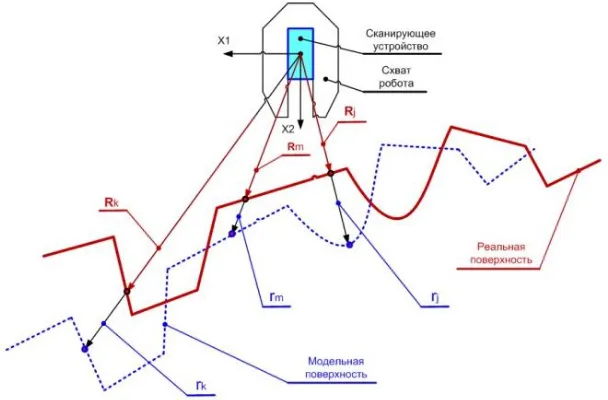
Therefore, to achieve the position of the task tool (gripper) relative to the external environment surface, which is identical to their relative “modeled” position, it is sufficient to additionally rotate and move the gripper (Fig. 1 represents the considerations above).
Fig. 1. Two-dimensional case of the external environment
For greater certainty figure 1 presents not three-dimensional, but two-dimensional case of the external environment. The positions vectors of the corresponding characteristic points of the real environment 𝑋𝑋((𝑅𝑅(, 𝜑𝜑() and its model 𝑥𝑥((𝑟𝑟(, 𝜑𝜑
2( ),
identified by locating devices, differ only in their radius vectors 𝑅𝑅(≠ 𝑟𝑟(, where 𝑖𝑖 =
1, 2, . . . , 𝑛𝑛 is the number of characteristic point.
In order for the position of the gripper relative to the real surface to be identical to the position of its model relative to the surface model, it is necessary that the position vectors of at least 2 characteristic points (in three-dimensional environment at least three characteristic points not lying on one straight line) be equal, i.e.
𝑋𝑋(= 𝑥𝑥(, where 𝑖𝑖 = 1, 2, . . . , 𝑛𝑛)
It is easy to prove that if for 3 points in three-dimensional environment position vectors coincide, then the equalities given above are valid for a larger number of corresponding characteristic points.
discrepancy 𝑥𝑥&(𝑡𝑡) − 𝑋𝑋(𝑡𝑡) between the desired and current positions of the task tool
relative to the surface of the external environment (in addition to the discrepancy functions of the generalized coordinates vectors 𝑔𝑔&(𝑡𝑡) and 𝑔𝑔(𝑡𝑡) and vectors of forces
interaction 𝐺𝐺&(𝑡𝑡) and 𝐺𝐺(𝑡𝑡), where:
𝑥𝑥9&= (𝑥𝑥9:, 𝑥𝑥9;, . . . , 𝑥𝑥9<), 𝑋𝑋 = (𝑋𝑋:, 𝑋𝑋;, . . . , 𝑋𝑋<)
4
Dynamic Analysis of the Control Process with Adaptation of
the Robot to the External Environment
The papers [7–13] present a detailed dynamic analysis of the robot control process with the use of in the control law the terms depending on the described above two types of discrepancy functions for the desired and current vectors of the generalized coordinates and the forces of interaction between the task tool and objects of the external environment.
This papers also present determined requirements for the structure and parameters of the control law, as well as the requirements for the construction parameters of the robot to maintain control efficiency, its stability while tracking the required movement trajectories of the task tool and while tracking the force of its interaction with environmental objects [16-25].
The stability of the control process must maintain with the complication of the control law by a new member depending on the vector of discrepancy between the desired and current positions of the task tool relative to the objects of its external environment.
To find the representation of this additional term maintaining stability of the control process, consider a functional that is square of module of the discrepancy function 𝐹𝐹 = |𝑥𝑥&− 𝑋𝑋|;.
Let us show that the control process is asymptotically stable if in the control law that additional term is a vector proportional to the anti-gradient of the functional [26-27].
The vector 𝑥𝑥&(𝑡𝑡) contained in 𝐹𝐹 is only time-varying function and is independent
of 𝑔𝑔. Therefore, an additional member of the control law proportional to the anti-gradient can be represented as:
𝑈𝑈AB?= −𝐾𝐾 E F𝜕𝜕𝑋𝑋 (
𝜕𝜕𝑔𝑔 H
I
(𝑥𝑥&( − 𝑋𝑋((𝑔𝑔)),
𝑖𝑖 = 1, 2, . . . , 𝑛𝑛 (1)
where JKLKNMOIis a transposed (3xn) functional matrix. As mentioned above, the modeled 𝑥𝑥&((𝑟𝑟
&(, 𝜑𝜑&(, 𝜃𝜃&() and real 𝑋𝑋((𝑅𝑅(, 𝜑𝜑6(, 𝜃𝜃6() position
Therefore, only the first non-zero coordinate remains in the three-dimensional vectors (𝑥𝑥&( − 𝑋𝑋((𝑔𝑔)). Then the vector (𝑥𝑥&( − 𝑋𝑋((𝑔𝑔)) can be represented in the more
compactly form:
𝑈𝑈AB?= −𝐾𝐾 E F𝜕𝜕𝑅𝑅 (
𝜕𝜕𝑔𝑔 H
I
(𝑟𝑟&(− 𝑅𝑅(),
𝑖𝑖 = 1, 2, . . . , 𝑛𝑛, (2)
𝜕𝜕𝑅𝑅(
𝜕𝜕𝑔𝑔 = 𝐴𝐴:𝐽𝐽,
where:
𝑟𝑟&(, 𝑅𝑅( are first components (radii) of position vectors 𝑥𝑥&(, 𝑋𝑋( of modeled and real
characteristic points;
KSM
KN is 1xn functional matrix (Jacobi-matrix) relating the incremental vector of the
generalized coordinates of the robot Δ𝑔𝑔 with incremental vector of spherical coordinates (Δ𝑅𝑅, Δ𝜑𝜑, Δ𝜃𝜃);
À1 is the first row of 3x3 matrix A relating the incremental vector (Δ𝑋𝑋, Δ𝑌𝑌, Δ𝑍𝑍) of Cartesian coordinates with the incremental vector of spherical coordinates
𝐽𝐽(= 𝐽𝐽 W( + 𝐽𝐽Y(
𝐽𝐽W(, 𝐽𝐽Y( are (3xn) blocks of the Jacobi matrix 𝐽𝐽(= Z[\
M
[]M ^ providing relation between
the angular velocity vector 𝑊𝑊 and the linear velocity 𝑉𝑉 of the coordinates origin of the gripper and the generalized velocity vector 𝑔𝑔.
𝑋𝑋a( is an oblique-angled matrix corresponding to the vector 𝑋𝑋( represented in the
Cartesian coordinate system related with the gripper. The dynamic description of the robot is as follows:
𝐴𝐴𝑔𝑔̈ + 𝐵𝐵𝑔𝑔̇ + 𝐷𝐷 = −𝑘𝑘g𝑘𝑘Nhi&𝐹𝐹 − 𝑘𝑘g𝑘𝑘Nhi&∑<(k:JKS
M
KNO I
(𝑟𝑟&(− 𝑅𝑅() (3)
𝐴𝐴 =𝜕𝜕𝑇𝑇𝜕𝜕𝑔𝑔 , 𝐵𝐵 =𝜕𝜕𝐴𝐴𝜕𝜕𝑔𝑔 −12 𝜕𝜕(𝑔𝑔̇𝐴𝐴)𝜕𝜕𝑔𝑔 + 𝐾𝐾&(m, 𝐷𝐷 = −𝜕𝜕𝜕𝜕𝑔𝑔
In (3) the control law component 𝑈𝑈 depending on the discrepancy functions (𝑔𝑔&−
𝑔𝑔) and (𝐺𝐺&− 𝐺𝐺) is omitted, since in [7] the authors propose the conditions for
stability of the robot control process with the use of this component. Therefore, the instability of the control process can be generated only by the component 𝑈𝑈AB? added
to the control law (2). For this purpose, it is useful to use new variables in the dynamic description:
Δ = (𝑔𝑔 − 𝑔𝑔n), Δ̇ = (𝑔𝑔̇ − 𝑔𝑔̇n), Δ̈ = (𝑔𝑔̈ − 𝑔𝑔̈n),
Consider the expression (3) to the representation in terms of the introduced variables Δ, Δ̇, Δ̈. This is well known to require to subtract the right and left sides of expression (3) in which the variables 𝑔𝑔, 𝑔𝑔̇, 𝑔𝑔̈ are replaced with 𝑔𝑔, 𝑔𝑔̇, 𝑔𝑔̈ of the same sides, in which 𝑔𝑔, 𝑔𝑔̇, 𝑔𝑔̈ are replaced with 𝑔𝑔o+ Δ, 𝑔𝑔̇o+ Δ̇, 𝑔𝑔̈o+ Δ̈.
Consider also the quasistationary mode, i. e.:
𝑔𝑔&(𝑡𝑡) ≈ 𝑐𝑐𝑐𝑐𝑛𝑛𝑐𝑐𝑡𝑡, 𝑋𝑋&(𝑡𝑡) ≈ 𝑐𝑐𝑐𝑐𝑛𝑛𝑐𝑐𝑡𝑡,
and therefore
𝑔𝑔o(𝑡𝑡) ≈ 𝑐𝑐𝑐𝑐𝑛𝑛𝑐𝑐𝑡𝑡, 𝑔𝑔̇o(𝑡𝑡) ≈ 𝑐𝑐𝑐𝑐𝑛𝑛𝑐𝑐𝑡𝑡.
As a result of this transformation, the dynamics equations in deviations after its linearization in the vicinity of values 𝑔𝑔o, 𝑔𝑔̇o take the following form:
𝐴𝐴oΔ̈ + 𝐵𝐵oΔ̇ + 𝑁𝑁oΔ + 𝑘𝑘g𝑘𝑘 ∑<(k:JKS
M
KNO IKSM
KNΔ = 0 (4)
where
𝐴𝐴o, 𝐵𝐵o are positively defined symmetrically constant matrices with a value 𝑔𝑔 = 𝑔𝑔o
which always occurs in mechanical system.
Symmetry and positive definiteness of 𝑁𝑁o follows from the fact that it is used for
estimation of the potential force near the equilibrium point 𝑔𝑔 = 𝑔𝑔o≈ 𝑐𝑐𝑐𝑐𝑛𝑛𝑐𝑐𝑡𝑡.
𝑘𝑘g𝑘𝑘 ∑<(k:JKS
M
KNO IKSM
KN is a symmetric and positively definite matrix (due to its
structure and scalarity of matrices 𝑘𝑘g and 𝑘𝑘).
Thus, in the resulting dynamics equation (4) which is a linear approximation of the initial nonlinear dynamic description of the behavior of the remotely controlled robot (3). All coefficients for variables Δ, Δ̇, Δ̈ are positively defined symmetric matrices. Consequently, this equation describes an asymptotically stable process, [7] which is easily proved by using the Lyapunov theorem.
Note the following useful feature of the proposed adaptive method of remote control: the fact that the characteristic points of the robot’s external environment are simple to be proposed, and their number is not regulated and can be changed in the process of control.
In comparison with other methods [4], this fact makes it possible to increase the reliability and quality of the control process, to smooth over and avoid possible control signal steps caused by “possible non-smoothness” of external surface.
The described process of implementing adaptive control is a process continuous in time. Indeed, after transferring the data generated during the training process to the local control system, it is simultaneously “processed” by the robot’s local control system until the end of the required operation. The generated data is:
• Programmed values of the time variation of the generalized coordinates vector 𝑔𝑔&((𝑡𝑡),
• Vectors 𝐺𝐺&((𝑡𝑡), of the force of interaction between the task tool and objects of
• The radii 𝑟𝑟&((𝑡𝑡) of the position vectors 𝑥𝑥&((𝑟𝑟&(, 𝜑𝜑&(, 𝜃𝜃&() of characteristic points from
external environment.
The control process is stopped only in case of emergency. Then, a corresponding message is sent to the central control center.
So-called discrete approach to implement the process of adaptive control is also possible. It differs adaptation process of the robot’s task tool to the possible inaccuracy of the modeled external environment which the robot is trained with.
The adaptation process is actually the process of implementing the algorithm for minimizing the discrepancy functional. Such algorithm can be an algorithm of mathematical programming, for example, the gradient one. The algorithm includes the following steps:
• Measurement of the current value of the generalized coordinates vector 𝑔𝑔&((𝑡𝑡).
• Measurement of the radii 𝑅𝑅(, where 𝑖𝑖 = 1, 2, . . . , 𝑛𝑛 are the first component of the
position vectors 𝑋𝑋( of the characteristic points, corresponding to the radii 𝑟𝑟 &( of the
position vectors 𝑥𝑥&( obtained from the control center.
• Anti-gradient of the discrepancy evaluation functional by the expression (2). • Move the robot by an amount Δ𝑔𝑔 proportional to the evaluated anti-gradient. • Check the value of the functional and the repetition of points 1....4 in case if the
functional is more than some predetermined small value, otherwise the end of the work.
As follows from the description of the adaptation process, its discreteness develops in the continuous movement of the robot at each step of the algorithm to calculate the value of the next movement Δ𝑔𝑔.
Note that using the gradient minimization algorithm implies that the magnitude of the gradient decreases as it approaches the zero minimum, i.e. when 𝑅𝑅( approaches to
𝑟𝑟&( as shown in (2) and, therefore, the step size decreases slowing down the control
process.
Therefore, to speed up the process, another method adapted to the peculiarities of the problem being solved is proposed to be used. This reduces finding an argument of the functional corresponding to its zero minimum, to an iterative process of solving algebraic equations by the Newton method.
In this case, these equations are formed by equating the discrepancy function to zero. Taking into account the identity of the angular coordinates of the position vectors of the corresponding characteristic points, this gives an equation of the form:
𝑟𝑟&= 𝑅𝑅((𝑔𝑔), 𝑖𝑖 = 1, 2, . . . , 𝑛𝑛, (5)
where 𝑟𝑟&= (𝑟𝑟&:, 𝑟𝑟&;, . . . . 𝑟𝑟&<),𝑅𝑅(𝑔𝑔) = (𝑅𝑅:, 𝑅𝑅;, . . . . 𝑅𝑅<).
Since the vector of generalized coordinates is six-dimensional, the necessary condition for a solution to the equation to exist is the six-dimensionality of the vectors 𝑅𝑅(, 𝑟𝑟
&(, i.e. it is necessary to use six characteristic points to implement the adaptation
To find the desired vector 𝑔𝑔 from (5) by using the Newton method, it is necessary to represent the differentiable vector-function 𝑅𝑅(𝑔𝑔) as a series of the vector Δ𝑔𝑔 terms in a certain neighborhood of the current value 𝑔𝑔 = 𝑔𝑔o, and only linear terms remain in
the expansion:
𝑟𝑟&= 𝑅𝑅(𝑔𝑔o) +KSKNΔ𝑔𝑔 (6)
If the functional matrix KS
KN presented by expression (6) is non-singular, then from
(6) it follows that:
𝐴𝐴N= JKSKNO u:
(𝑟𝑟&− 𝑅𝑅(𝑔𝑔o)) (7)
The value 𝑔𝑔v= 𝑔𝑔
o+ Δ𝑔𝑔 is the first approximate value of the desired argument 𝑔𝑔.
The second approximation is found from (6) by replacing the value 𝑔𝑔o by obtained
value 𝑔𝑔v . The process continues until the discrepancy function reaches a
predetermined small value. At each step, the robot is moved by the obtained value Δ𝑔𝑔 until the descrepancy function reaches a specified small value.
5
Conclusion
In the article, a method for implementing remote bilateral control of space robots is proposed. The approaches given in [7-13] are developed, which increases possibility of successful implementation of sustainable remote control by a manipulation robot operating in the environments with varying topography.
The control process consists of the following steps:
• With the help of a video camera and a scanning three-dimensional locator, the “topography” of the external environment in which the remote-controlled robot should function is formed. In other words, the coordinates of points on the surface of external environment in the coordinate system of the scanning device, for exam-ple, spherical, are determined with a certain scanning step.
• A three-dimensional model of the external environment is created in the control center of the robot. It can be full-scale or combined, consisting of full-scale and virtual elements "joint" with each other using augmented reality technology. • To perform the required operation the robot is trained by a human operator in this
modeled environment by using a robot model preferably a physical (full-scale) one. For this purpose, the human operator performs the required operation with the use of the mode of bilateral control of the robot model.
movement can be limited to constraints (for example, when performing assembly operations).
• In addition, the number of generated data includes the laws of time variation for the vector of characteristic points on the surface of external environment to correct the position of the robot’s task tool in relation to objects of the external environment. • Perform the desired operation by the robot.
6
References
[1]Anderson R., Spong M. Bilateral Control of Teleoperators with time Delay // IEEE Trans.
on Automatic Control. 1989. V. 34, No. 5. P. 494–501. https://doi.org/10.1109/9.24201
[2]Hokayem P., Spong M. Bilateral Teleoperation: An Historical Survey // Automatica. 2006.
V. 42. P. 2035–2057. https://doi.org/10.1016/j.automatica.2006.06.027
[3]Niemeyer G., Slotine J. Stable Adaptive Teleoperation // IEEE J. Oceanic Engineering.
1991. V. 16(1). P. 152–162. https://doi.org/10.1109/48.64895
[4]Fite K., Goldfarb M., Rubio A. Transparent Telemanipulation in the Presence of Time
De-lay // Proc. IEEE/ASME Intern. Conf. on Advanced Intelligent Mechatronics 1. Port
Is-land, Kobe, Japan. 2003. P. 254–259. https://doi.org/10.1109/AIM.2003.1225104
[5]Park J., Cho H. Sliding-mode Control of Bilateral Teleoperation Systems with
Force-reflection on the Internet // Proc. IEEE/RSJ Intern. Conf. on Intelligent Robots and
Sys-tem. V. 2. Takamatsu, Japan. 2000. P.1187–1192. https://doi.org/10.1
109/IROS.2000.893180
[6]Garcia-Valdovinos L., Parra-Vega V., Arteaga M. Observer-based Higher-order Sliding
Mode Impedance Control of Bilateral Teleoperation Under Constant Unknown Time De-lay // Intelligent Robots and Systems, IEEE/RSJ Intern. Conf. Beijing, China. 2006. P. 1692–1699.
[7]F.M.Kulakov Metods of Supervisory Remote Control over Space Robots (2018) Journal of
Computer and Systems International, 2018, Vol. 57, No.5,pp. 822-839. DOI:. 10.1134/S1064230718050088
[8]Kulakov F., Alferov G.V., Efimova P., Chernakova S., Shymanchuk D. Modeling and
Control of Robot Manipulators with the Constraints at the Moving Objects (2015) 2015 Intern. Conf. "Stability and Control Processes" in Memory of V.I. Zubov ,SCP 2015
-Proceedings, P.7342075, pp. 102-105. https://doi.org/10.1109/SCP.2015.7342075
[9]Alferov G.V., Malafeyev O.A. The Robot Control Strategy in Domain with Dynamical
Obstacles (1996) Lecture Notes in Computer Science. (including subseries Lecture Notes in Artificial Intelligence and Lecture Notes in Bioinformatics), 1093, pp. 211-217. https://doi.org/10.1007/BFb0013961
[10]Kulakov F., Alferov G., Efimova P. Methods of Remote Control over Space Robots (2015)
2015 Intern. Conf. on Mechanics - Seventh Polyakhov’s Reading, P. 7106742. https://doi.org/10.1109/POLYAKHOV.2015.7106742
[11]Kulakov F., Alferov G., Sokolov B., Gorovenko P., Sharlay A. Dynamic analysis of space
robot remote control system (2018) AIP Conference Proceedings, 1959, P. 080014. https://doi.org/10.1063/1.5034731
[12]Kulakov F., Sokolov B., Shalyto A., Alferov G. Robot Master Slave and Supervisory
Con-trol with Large Time Delays of ConCon-trol Signals and Feedback (2016) Applied
[13]Kulakov F., Kadry S., Alferov G., Sharlay A. Bilateral Remote Control over Space
Manip-ulators (2018) AIP Conference Proceedings,. 2040, P.150015 https://doi.org/10.1
063/1.5079218
[14]D. V. Shymanchuk On the coupled orbit-attitude control motion of a celestial body in the
neighborhood of the collinear libration point L1 of the Sun-Earth system, in 2017 Con-structive Nonsmooth Analysis and Related Topics (Dedicated to the Memory of V.F. De-myanov), CNSA 2017 - Proceedings IEEE Conference Proceedings CFP17L17-ART, edit-ed by L. N. Polyakova (Institute of Electrical and Electronics Engineers, Saint Petersburg, Russia, 2017), pp. 1–-4.
[15]Shymanchuk D. V. Modeling of controlled coupled attitude-orbit motion in the
neighbor-hood of collinear libration point L_1. Vestnik of Saint Petersburg University. Applied mathematics. Computer science. Control processes, 2017, vol. 13, iss. 2, pp. 147-167.
[16]Kadry, S., Alferov, G., Ivanov, G., Sharlay, A. About stability of selector linear differential
inclusions. (2018) AIP Conference Proceeding, 2040, P.150013. https://doi.org/10.1
063/1.5079216
[17]Kadry, S., Alferov, G., Ivanov, G., Sharlay, A. Stabilization of the program motion of
con-trol object with elastically connected elements. (2018) AIP Conference Proceedings, 2040,
P.150014. https://doi.org/10.1063/1.5079217
[18]Ivanov,G., Alferov,G.,Gorovenko,P., Sharlay,A. Estimation of periodic solutions number
of first-order differential. equations. (2018) AIP Conference Proceedings, 1959, P.080006, https://doi.org/10.1063/1.5034723
[19]Seifedine Kadry, Gennady Alferov, Gennady Ivanov, and Artem Sharlay Almost Periodic
Solutions of First-Order Ordinary Differential Equations. Mathematics, 2018 V.6, No9, P.171, DOI: 10.3390/math 6090171
[20]Alferov,G.V., Ivanov,G.G., Efimova,P.A., Sharlay,A.S. Stability of linear system with
multitask right-hand member (2018) Stochastic Methods for Estimation and Problem Solv-ing in EngineerSolv-ing, pp. 74-112. DOI; 10.4018/978-1-5225-5045-7.ch004
[21]Alferov,G., Ivanov,G., Efimova,P., Sharlay,A. Study on the structure of limit invariant sets
of stationary control systems with nonlinearity of hysteresis type (2017) AIP Conference
Proceedings, 1863, P.080003. https://doi.org/10.1063/1.4992264
[22]Alferov,G.V., Ivanov,G.G., Efimova,P.A. The structural study of limited invarie sets of
re-lay stabilized systems. (2017) Mechanical Systems: Research, Applications and Technolo-gy, pp.101-164. Book Chapter.
[23]Ivanov,G., Alferov,G., Efimova,P. Integrability of nonsmooth one-variable functions.
(2017) 2017 Constructive Nonsmooth Analisis and Related Topics (Dedicated to the
Memory of V.F. Demyanov), CNSA 2017- Proceedings, P.7973965 https://doi.org/10.1
109/CNSA.2017.7973965
[24]Alferov,G.V., Gorizontov,A.M. Resource Management in Flexible Automated Production.
(1987) Kibernetika I Vychislitel’naya Tekhnika, 73, pp.76-81.
[25]Efimova P., Shymanchuk D. Dynamic model of space robot manipulator, Applied
Mathe-matical Sciences, Vol. 9, Iss. 93-96, 2015, pp. 4653-4659, https://doi.org/10.1
2988/ams.2015.56429
[26]Ivanov,G., Alferov, G., Sharlay,A., Efimova,P. Conditions of asymptotic stability for
line-ar homogeneous switched systems. (2017) AIP Conference Proceedings, 1863, P,080002, https://doi.org/10.1063/1.4992263
[27]Kurochkin V., Shymanchuk D. Positional control of space robot manipulator. (2018) AIP
7
Authors
F.M. Kulakov, St. Petersburg Institute of Informatics and Automation of the
Rus-sian Academy of Sciences (SPIIRAN), 14 line 39, 199178, Saint Petersburg, Russia.
S. Kadry, Department of mathematics and computer science, Faculty of science,
Beirut, Lebanon.
G.V. Alferov, Saint Petersburg State University, Universitetskaya nab.7-9, 199034, Saint Petersburg, Russia.
P.A. Efimova, Saint Petersburg State University, Universitetskaya nab.7-9, 199034, Saint Petersburg, Russia.