Do the rich consume higher quality goods 100216.pdf

Do the rich (really) consume higher quality goods?

Evidence from international trade data

Vincenzo Merella

Daniel Santabárbara

February 2016

Abstract

Using average import prices as proxies for quality, a large body of the international trade literature …nds both theoretical and empirical support to the positive relationship between importer income and quality of imports. Several authors, however, argue that the empirical evidence on the link between income and product quality might be spurious, since import prices (unit values) could be a¤ected by other factors than product quality. Building on Khandelwal’s (2010) discrete choice model approach, where quality is inferred by quanti-tative market shares as well as unit values, we develop a model that allows for willingness to pay for quality to vary with income. Using this alternative framework, we empirically validate the theoretical relationship between importer income and product quality by using the Eurostat’s COMEXT database, which collects customs data reported by EU countries at 8-digit disaggregation. Our estimations support the positive link between consumer income and product quality, which is also generally stable across sectors.

Keywords: export quality, import shares, unit values, nested logit demand JEL Classi…cations: F12, F14, L15

We would like to thank the seminar participants at the Bank of Spain and at the 2013 SAEe meeting (CEMFI-UIMP, Santander) for the useful comments. This paper has been written while Vincenzo Merella was a Research Fellow at the Bank of Spain, whose …nancial support is kindly acknowledged.

y_{University of Cagliari and BCAM. Mailing address: Department of Economics and Business, Viale}

Sant’Ignazio 17, 09123 Cagliari, Italy. Email: [email protected].

z_{Bank of Spain. Mailing address: International Economics Division, calle Alcalá 48, 28014 Madrid. EMail:}

1

Introduction

Understanding the determinants of import structure is a fundamental concern of the international trade literature. A growing number of contributions posit a prominent role of product quality in shaping importer behavior. In this paper, we develop a model in which richer consumers demand goods of higher quality and, departing from the assumption that information on quality is embedded only in prices, we empirically test the model predictions using disaggregated trade data.

The in‡uence of the relationship between product quality and consumer income on consumer demand, if substantiated by empirical evidence, would have major consequences on the inter-national markets. Arguably, the exporters choice of how to di¤erentiate their products when dealing with rich importers seeking high quality goods might di¤er substantially from the one they would opt for when dealing with poorer importers. Likewise, the e¤ectiveness of a given trade policy might dramatically change depending on the type of competition that domestic pro-ducers face internationally. The aim of this paper is to contribute to shed light on the structure of international demand by providing novel evidence on the link between quality of exports and importer income.

In a number of recent theoretical contributions, the relationship between product quality and consumer income is regarded as an important determinant of import and export ‡ows [e.g., Flam and Helpman (1987); Murphy and Shleifer (1997); and, more recently, Fajgelbaum, Grossman and Helpman (2011); Jaimovich and Merella (2012, 2015)]. In all these articles, the main prediction is invariably the following: richer importers tend to trade more with exporters producing higher quality goods. The link between quality of exports and importer income appears to …nd support in a large empirical literature: product quality correlates positively with consumer income [e.g., Hummels and Klenow (2005); Hallak (2006); Bastos and Silva (2010); Flach (2014)]. The extent to which such empirical …ndings relate to the theoretical prediction is, however, controversial. The crux of the matter is that observed average import prices are typically used as proxies for the quality levels of the consumption goods.

country (importer). The rationale for using a unit value as a proxy for quality hinges on a number of arguments: e.g., higher quality goods would require more costly inputs, hence be more expensive; a market price di¤erential between two similar goods may hold only if their quality levels di¤er. Several authors, however, argue that the correlation between prices and income may actually be determined by factors other than quality [e.g., Hallak and Schott (2011); Simonovska (2010)]. The most immediate argument is that goods sourced from di¤erent countries may command heterogeneous tari¤s and trade costs. Furthermore, exporters may charge varied markups in di¤erent markets (pricing-to-market), which could lead to systematically higher prices charged in more developed economies. Finally, even products that are regarded as close substitute may exhibit some distinctive characteristics, which could result in a certain residual degree of horizontal di¤erentiation.

Building on this criticism, part of the literature attempts to construct alternative measures of quality that do not rely solely on prices. For example, Khandelwal (2010) and Pula and Santabárbara (2012) use quantitative market shares to obtain measure of quality for the goods exported by a given country; Hallak and Schott (2011) bring in trade balances. The idea behind these two approaches is to extract information on quality from trade volumes holding prices constant, building on the intuition that consumers care about price relative to quality in choosing among products. Hence, two goods with the same price but di¤erent trade volumes should have di¤erent levels of quality.

This paper follows (by gathering information on quality from volumes of trade and import prices) and extends (by letting willingness to pay for quality rise with income) the …rst of these two approaches. We use a nested logit demand system to infer information on quality from quantitative market shares as well as import prices. Consumers face a set of vertically and horizontally di¤erentiated goods, produced by monopolistically competitive …rms. They have objective taste for quality, whose di¤erent levels are identi…ed on the vertical dimension, and idiosyncratic tastes for the speci…c characteristics that horizontally di¤erentiate products with the same level of quality. To this standard features, we add a preference representation where willingness to pay for quality rises with income. Therefore, our framework allows for the valuation of quality to be income-dependent.

richer importers purchase their goods from exporters producing higher quality products. The novel feature in our approach is how this theoretical prediction is validated empirically. Instead of studying the link between importer income and average import price, we investigate the rela-tionship between importer income and the quality derived from comparing products’quantitative market shares and prices.

To test whether a positive correlation importer income and our measure of product quality exists, this paper exploits the unique features of the Eurostat’s COMEXT database, which provides information on each EU member state’s imports from 240 partner economies at the CN-8 digit product level (approximately CN-8500 product headings). This information is used to obtain a highly disaggregate measure of the quality levels of the products (for each 8-digit product and every exporter) imported by each EU country. The underlying strategy is to consider di¤erent members of the EU as consumers operating in a single market. We can then test the relationship between quality and income using countries GDP per capita. Our estimates suggest a robust positive correlation between income and product quality. Speci…cally, as we illustrate in Section 3, our results are robust to di¤erent speci…cations, do not rely on any particular industry, and are also robust to a number of controls and alternative instrumentation strategies.

Related literature

A large strand of the literature provides evidence of a positive correlation between quality of imports and importer GDP. Using cross-sectional data for bilateral trade among 60 countries in 1995, Hallak (2006) shows that rich economies tend to import relatively more from exporters that produce high-quality goods. Fieler (2011) uses an even richer dataset (about 160 countries in the period 1995-2007) to illustrate the positive link between income per capita growth and the rise in quality levels. Choi, Hummels and Xiang (2009) exploit household income data (26 countries in 2000) and document that di¤erent quality distributions map into di¤erent income distributions, in a way that is consistent with rising willingness to pay for quality.1

The common feature of all these contributions is that unit values are used as proxies for quality levels. Several studies point out that unit values may capture other links to the importer’s

1_{Further evidence that richer consumers typically purhcase product of higher quality can be found, for example,}

income per capita than product quality. Khandelwal (2010) argues that import prices may re‡ect variations in manufacturing costs, and expensive goods may be traded only because they exhibit particular features that match idiosyncratic preferences of a small fraction of consumers in the destination country. Simonovska (2010) investigates the role of pricing-to-market in determining import prices and, using data on prices of more than two hundreds identical goods sold in about thirty countries, shows that variable mark-ups account for up to a third of the observed cross-country price di¤erentials.2 _{In addition, heterogeneity in tari¤s and transportation costs are a}

well documented source of di¤erences in the prices of tradables. For these reasons, we choose to depart from the existing literature investigating the link between quality and per capita GDP by adopting an alternative measure of quality, and study the relationship between consumer income and product quality inferring the latter from the relative volumes traded in the international markets.

There are two main approaches in the literature that attempt to construct alternative quality measures. On the one hand, Hallak and Schott (2011) infer relative product quality by positing that countries with trade surpluses o¤er higher quality than countries running trade de…cits, holding observed import prices constant. On the other hand, Khandelwal (2010) deduces quality levels by exploiting trade volumes, postulating that higher-quality products attract higher market shares, conditional on price. We choose to follow more closely the second approach, because the richness of observations in our dataset allows for a …ner detailed analysis than that based on world-level exports.3 _{Hence, our paper di¤ers from Hallak and Schott (2011) as we infer}

product quality by exporter at the sectoral level rather than looking at each country as a whole. Furthermore, we depart from both approaches in that we explicitly let willingness to pay for quality rise as consumer income increases. This feature represents the main novelty of our paper relative to the existing studies in this literature.

Finally, our paper relates to those contributions building on the tradition of models with a nested logit demand structure, …rst proposed by McFadden (1973), and later developed by

2_{Alessandria and Kaboski (2011) provide further evidence of this phenomenon, showing that US exporters}

ship the same good to low-income countries at lower prices.

3_{We are aware that a “disadvantage is that [. . . ] one-way ‡ows to a single country are likely to be substantially}

Berry (1994) and Berry, Levinsohn, and Pakes (1995). These modeling has been applied to international trade by Goldberg (1995) and Verboven (1996) and, more recently, by Verhoogen (2008) and Khandelwal (2010). Here, we extend these works by introducing a mechanism that leads to a link between product quality and consumer income. It is worth noting that Fajgelbaum, Grossman and Helpman (2011) also introduce willingness to pay for quality in a model with a nested logit demand system. Their focus, however, is very di¤erent from ours. Their study is exclusively theoretical, and aims to explain why richer countries export higher-quality goods, whereas our quantitative model is designed to provide measures of product quality to test the link between the latter and consumer income.4

The remaining of the paper is organized as follows. Section 2 illustrates the model from which we derive our predictions. Section 3 discusses our empirical strategy, and shows that our estimations support the theoretical predictions of the model. Finally, section 4 concludes.

2

Theoretical framework

This section builds on the tradition of the nested logit discrete choice models.5 Most features of our model are standard: (i) we consider a partial equilibrium world economy where a large number of independent markets exist; (ii) throughout the whole theoretical analysis, we restrict our attention to a single, representative, market;6 _{(iii) products are potentially sourced from,}

and destined to, several countries: to simplify matters, we only consider two source countries, denoted N and S, and two destination countries, denotedH and L. The only novel feature of our approach is to allow for willingness to pay for quality to rise with income.

Within every source country there is a unit mass of …rms, indexed by j, each producing a di¤erentiated good. Labour inputs are immobile (which allows for di¤erent wages in N and

S) and technologies di¤er across countries. We assume that country N enjoys higher wages (wN > wS) and technological capabilities (AN > AS) than countryS. Every destination country 4_{In fact, the divergence in the goal of the two papers entails a fundamental di¤erence in the modelling strategy.}

Fajgelbaumet al.(2011) develop a general equilibrium model where idiosyncratic tastes have a generalized extreme value (GEV) distribution. We opt for a partial equilibrium model with idiosyncratic tastes having a type I extreme value distribution.

5_{For a textbook description of this model, see Tirole (1988).}

6_{The arguments discussed here naturally extend to all sectors considered in our empirical investigation, which}

is populated by a unit mass of consumers. The two countries di¤er in their income levels and (possibly) size, and we assume that country H is richer (yH > yL) than country L. Size is

denoted by and expressed in relative terms, hence the destination region has size one, and

L 1 H. Two additional features complete the model. First, outside sectors determine

wages and incomes. Second, domestically produced outside varieties are available to consumers in each destination country.

By di¤erentiating their products, …rms in the source region engage in monopolistic competi-tion. They exercise their degree of market power by setting the prices of their products taking consumer demand into account. For this reason, we begin our analysis by studying consumer choice. Each individualiin countryM =_fH; L_gmay consume one unit of a di¤erentiated good

(j; X), produced by …rmj in countryX=_fM; N; S_g. Good(j; X)in M is characterized by the quality levelqM

j;X (which is agreed upon by all consumers) and by the horizontal di¤erentiation

term"i;M_j;X (whose valuation is instead consumer-speci…c).

Valuation of good (j; X) by consumer i in country M is represented by the indirect utility function:

V_j;Xi;M = Mq_j;XM pM_j;X+"i;M_j;X (1) where M re‡ects the country-M consumers’(common) valuation for quality,pM

j;X is the price of

good(j; X)when traded in countryM, and represents consumers’(worldwide common) price sensitivity. We introduce the concept of rising willingness to pay for quality as income increases by assuming that valuation for quality is an increasing function of income.

Assumption Valuation for quality M (yM)is such that (0)>0and@ (yM)=@yM >0.

As a result, the largeryM, the higher M, and the greater the willingness to pay for quality, all

other conditions holding constant.

Under the assumption that the horizontal term "i

j;x follows a Gumbel distribution, the

ex-pected aggregate demand for good(j; X)by countryM is:

cM_j;X = M

exp Mj;X

P

Y=fM;N;Sg

R1 0 exp

M

k;Y dk

where M_j;X MqM

j;X pMj;X represents the average valuation of good (j; X) in country M,

which is independent of n"i;M_j;Xo since idiosyncratic elements vanish when aggregating across consumers.7

In each country of the source region, …rms compete by producing vertically and horizontally di¤erentiated goods. Vertical di¤erentiation consists of choosing a particular quality version of the supplied good. To produce one unit of quality q, a …rm in country X faces the cost

wX+q2=(2AX). (Recall thatAX is a technological parameter; wageswX are determined by an

outside sector and therefore exogenous.) Horizontal di¤erentiation consists of choosing whether to embed speci…c characteristics to further personalize the supplied good. All …rms horizontally di¤erentiate goods at no additional cost.

Each …rmj in countryX take country-M consumer demand (2) into account when choosing pricepM

j;X and qualityqMj;X to maximize pro…ts: M

j;X = max_p;q p wX q2

2AX

Mexp Mq p

P

Y=fM;N;Sg

R1 0 exp

M

k;Y dk

(3)

(Atomless) …rms cannot in‡uence the equilibrium allocations, hence the optimal price charged is:

pM_j;X = 1 +wX+ qM

j;X

2

2AX

(4) the optimal quality is:

q_j;XM =

M AX

(5) and the (average) valuation of good(j; X)in countryM:

M

j;X =

M 2_A

X

2 1 wX (6)

From (4)-(6), we may note that: (i) all …rms in each source country optimally supply to country M goods of the same quality level (q_j;XM = q_XM, ₈j), which are hence equally priced (pM

j;X =pMX, 8j) and, on average, equally valued ( M

produced inN are always of higher quality, and given larger valuation, than those produced in

S; (iii) by replacing (5) into (4) in turns out thatpM

X =wX+ M

2

AX= 2 2 + 1= and, since wN > wS, goods produced inN are also more expensive than those produced inS.8

Recall that valuation for quality is an increasing function of consumer income. Considered in conjunction with (5), this feature of the model delivers the central prediction of our model, which we may summarize as follows.

Proposition. Goods sourced from countryX to the destination countryH are always of higher quality than those sourced toL:

qH_X > q_XL; ₈X

Proof. The result immediately follows from noticing that, since yH > yL, then H > L and qH_X = HAX= > LAX= =qXL.

This result implies that richer consumers (highery), displaying higher willingness to pay for quality (larger ), have a di¤erent spending structure than poorer consumers and, in particular, tend to import higher quality goods. The central prediction of our model is therefore in line with those found in the literature: product quality and consumer income should be positively related. The novel feature in our approach is how this theoretical result translates into an empirical test. As we discussed in the previous section, empirical contributions investigating the correlation between importer’s income and consumption goods quality typically use unit values (average import prices) as proxies for quality. We depart from the literature and infer product quality from (quantitative) market shares in a direct fashion, once unit values are controlled for.

In order to o¤er a more accurate description of the link between theoretical prediction and empirical test, it proves convenient to derive how import volumes translate into quantitative market shares, relative to the domestic market share. To do so, …rst notice that we may obtain total consumptioncM _{in the destination countryM by summing up aggregate demand (2) across}

source countries:

cM X

X=fM;N;Sg M

exp M_X P

Y=fM;N;Sgexp

M Y

= _M

We then derive the market share of the source country X in the destination country M by computing the ratio between the relevant aggregate demand and total consumption:

sM_X c M X cM =

Mexp MX

P

Y=fM;N;Sgexp

M Y

1

M

=

exp M_X P

Y=fM;N;Sgexp

M Y

(7)

Following the literature, we can further simplify this expression by normalizing to zero the average valuation of the domestically produced goods(j; M), which amounts to imposing M_M =

M

q_MM pM_M = 0. Using (7), the domestically produced goods market share is:

sM_M =

exp M_M P

Y=fM;N;Sgexp

M Y

=_P 1

Y=fM;N;Sgexp

M Y

(8)

As a result, the relative quantitative market share of the source country X in the destination countryM is given by the ratio of (7) to (8):

sM_X sM M

=

exp M_X P

Y=fM;N;Sgexp

M Y

0

@_P 1

Y=fM;N;Sgexp

M Y

1 A

1

= exp M_X (9)

Taking logarithms, and using the de…nition of average valuation for good(j; X)in the destination countryM to substitute for M_X, we obtain the equation that we bring to the data in order to infer our measure of product quality:

lnsM_X lnsM_M = M_X = M_X pM_X (10) where M

X M

qM

X = lnsMX lnsMM + pMX is the observationally relevant variable.9

This result, implied by the logistic nature of the model, represents the cornerstone of this type of models. From an empirical point of view, since quantitative market shares and prices are observable whereas qualities are not, the latter may be inferred by market shares once the

9_{This de…nition is due to the impossibility to identify} M _andqM

X separately. This caveat does not represent

a major issue, since: (i) M is the same for all goods imported by a given country, hence it works as a mere scale factor applied to a measure that is ordinal by nature; (ii) when comparing goods imported by di¤erent regions, this scale factor only magni…es the di¤erence between (ordinal) quality levels; the mapping between qM

X and M_qM

X is monotonic sinceq M

e¤ect of price is accounted for. In this respect, the novelty of our analysis lies in investigating the relationship between consumer income and product quality within this framework, where the newly developed measures of quality replace average import prices as proxies for quality.

3

Empirical approach

As we have shown in the previous section, our model predicts that the quality embodied in each traded good is an increasing function of consumer income. This prediction can be empirically tested using (10). Since market shares and prices are observable, quality may be inferred by (quantitative) market shares once the price e¤ect is accounted for. In what follows, we …rst illustrate the data that we use to test our prediction. We then discuss how we develop our estimations. Finally, we present our empirical results.

3.1

Dataset and estimation strategy

We estimate the demand function (10) for each good using data from the Eurostat’s COMEXT database. The COMEXT database collects EU harmonized customs data and contains informa-tion on all trade ‡ows reported by each EU country. It is a disaggregated data source, which provides trade data at the CN8-digit product level.10 _{In particular, this database contains values}

and quantities of all imports for each EU country. For a more homogeneous data availability and to obtain a properly balanced panel, in our empirical exercise we consider …ve developed countries among the EU members, namely: Germany, France, Italy, Spain and the UK.11

Accord-ingly, our database is four dimensional: it contains import data for 5 destination EU countries (M) under 8500 product labels (g) from 240 trade partners (X) for the 1995-2007 period (t). In what follows, we denote the good imported under product labelg from countryX as a variety

z= (g; X). As such, in our analysis a variety can be seen as the basic unit of consumer choice.12

1 0_{For example, we are able to distinguish within the men’s knitted shirt category (CN 4 digit code 6105) by}

material: cotton (61051000), synthetic …bre (61052010), arti…cial …bre (61052090), wool (61059010), or other material (61059090).

1 1_{These …ve countries are the largest markets within EU, which guaratees that they import a comparable set of}

products from their trade partners. Besides, the selected countries are among the richest in the world (the relevant per capita GDP …gures are well above 30,000 international dollars; source: World Bank, 2013), and display fairly similar income distributions (e.g., the relevant Gini coe¢ cients range from 0.28 to 0.35; source: Eurostat, 2012).

1 2_{Note that horizontal di¤erentiation, as discussed in the previous section, occurs at the product level. As a}

In order to guarantee a certain homogeneity in the demand function for the di¤erentiated products, we estimate a separate demand function for each NACE 4-digit industry.13 _{In our}

analysis, all industries with undi¤erentiated products are dropped, as bulding a quality ladder in such industries would make little sense: those industries are selected using Rauch’s (1999) di¤erentiated products classi…cation. Table 1 gives an overview of the database at a 2-digit level. Overall, the database contains 189 four-digit industries, but data availability reduces the number of separate equations we can actually estimate to around 160. On average, per equation, we have 30 productsg, around 2000 varietieszand nearly 28000 observations(z; t). The coverage of the database varies signi…cantly across the 2-digit industries. For example, wearing apparel has on average 56 products per equation, while the o¢ ce machinery industry has only 16.14

X.

1 3_{Each 4-digit NACE industry is linked to the relevant CN 8-digit classi…cation through appropriate}

corre-spondence tables provided by EUROSTAT.

1 4_{While it is apparent that our estimates are based on a large but not particularly balanced panel of data, this}

Taking all the speci…cs of our database into consideration, we can rewrite (10) in the following form:

lnsz;t lns0;t= z+ t+ M + y pz;t+ lnnsz;t+ z;t (11)

This is the equation that we ultimately estimate separately for each NACE 4-digit industry. In each destination country,sz;tmeasures the market share of varietyzrelative to total consumption

of goods in the relevant 4-digit industry, in turn computed as the sum of domestic production and imports, minus exports.15 _{The market share is calculated in quantitative terms. We also}

consider an outside variety, required in the demand system, as the domestic substitute for imports in each country, whose market share,s0;t, is calculated as one minus the industry’s overall import

penetration at 4-digit.

In equation (11), we estimate market quality M

X as a sum of four components: the time

invariant component of quality ( _z) is measured by a variety …xed e¤ect; the common shock ( _t) is calculated as a year …xed e¤ect; a destination country dummy ( M) controlling for idyosincratic

features; the income e¤ect, y lnyM, obtained by introducing destination per-capita GDP as

a regressor in (11); …nally, the term ( _z;t) that is unobserved and is obtained from the estimation error. Intuitively, equation (11) shows that a larger market share is related to higher quality after controlling for the variety’s relative price. Most importantly for our analysis, our model predicts that product quality increases with consumer income and, therefore, we expect >0.

The demand function (11) allows for di¤erent degree of substitutability across products. The nested logit speci…cation of the demand curve assumes di¤erent substitability patterns among groups of varieties or ’nests’, which however have to be determined ex-ante. We let product labelsgserve as nests. In particular, it is assumed that varieties within the same product exhibit a higher degree of substitutability than varieties of di¤erent products. For example, a Chinese cotton shirt is more substitutable with a Vietnamese cotton shirt than with a Chinese nylon shirt.16 _{The nest term ns}

z;t is calculated as the import share of variety z in the total imports

of product g (the nest).17 _{It is introduced to limit the extent of the issues arising from the} 1 5_{The sectoral level is chosen at NACE 4-digits since this is the most disaggregate level at which data is}

available for calculating market shares in consumption.

1 6_{In this example, cotton shirts and nylon shirts are two distinct nests.}

1 7_{Theoretically,nsz;tshould be calculated as a market share in consumption. However, given that we have no}

independence of irrelevant alternatives in traditional logit models.

The substitution parameter can be interpreted as follows. As approaches one, there will be perfect substitution among varieties within the nest (e.g. between Chinese and Vietnamese cotton shirts), but no substitution across nests (e.g. no substitution between cotton and nylon shirts). As a result, if the price of a given variety increases, consumers will substitute it with varieties from the same nest but not from other nests. This implies that the varieties’ relative market share will change within the nest, but not outside of the nest, and thus changes in the overall market share sz;t will be exclusively determined by the market share nsz;t within the

nest.18 _{In fact, in the case of an increase in its relative price, a variety that is easier to substitute}

will have a stronger decline in its market share, even if no change occurs in its relative quality. Given that the price pz;t and the nest term nsz;t are endogenous, i.e., contemporaneously

correlated with the residual _z;t, in order to obtain consistent estimates of (11), we consider a number of instruments. For the unit values, pz;t, we use two sets of instruments. Given that

the COMEXT database contains neither variety-level transportation costs nor non-rival variety characteristics (which are widely used instruments in the literature since Hausman, 1997), our …rst set of instruments relies on non-variety speci…c instruments, and in particular on country level data, namely the bilateral exchange rate and a proxy for transportation costs calculated as the interaction of bilateral country distances and the oil price.19 _{This set of instruments has}

the advantage of being available for the whole sample. The second set of instruments is variety-speci…c, and consist of the varieties’ average unit values on alternative EU markets. The idea behind using these so called Hausman instruments is that changes in unit values in third markets (e.g., Belgium when Germany is considered) can be assumed to re‡ect cost shocks and thus be used as instruments for prices with regard to the EU member state market under consideration. In addition, the sustitution parameter, , is instrumented with the number of varieties within the nest and the number of varieties exported by a country.

the share of varietyz import in the total imports of productg. This is equivalent to the assumption that each product market has the same import penetration ratio.

1 8_{As an example, if the price of the Chinese cotton shirt goes up, consumers will substitute it with Vietnamese}

cotton shirts and not by Chinese nylon shirts. The overall market share of both cotton and nylon shirts will remain unchanged while the market share of Chinese cotton shirt within the apparelsector will fall together with its market share within the cotton shirtnest.

1 9_{Bilateral exchange rates are taken from IFS database, distances are from the CEPII database}

In what follows, we compare the results obtained using three methods: the ordinary least square estimation (labelled ‘OLS’), which does not deal with endogeneity issues; an instrumental variable estimation making use of the subset of non-variety-speci…c instruments only (labelled ‘IV1’); and an instrumental variable estimation using the full set of variety and non-variety speci…c instruments (labelled ‘IV2’).

3.2

Estimation results

To give an overview of the goodness of the regressions, Table 2 shows a summary of the estimation results, focusing on the coe¢ cient of our variable of interest, i.e., the log of per capita GDP (hereafter, GDP coe¢ cient).20 _{Given the large number of separate equations, one per 4-digit}

industry, the table shows the distribution of the coe¢ cients and the associated p-values across our estimations.21 From top to bottom, the three boxes in Table 2 illustrate the results of the OLS estimation and of the two sets of IV estimations, the …rst one considering only non-variety speci…c instruments (IV1), and the second one with the full set of instruments (IV2). Hereafter, unless otherwise stated, we refer to the IV2 approach as the benchmark estimation, since it deals with endogeneity with a better set of instruments.

As expected, the mean of the GDP coe¢ cient is positive in all di¤erent estimation strategies, suggesting that richer countries’ consumers tend to purchase higher quality goods from their trade partners. The average magnitude of the coe¢ cient is sizeable (about 1:6). The result of our estimations is not driven by just a few industries: across the 159 estimated equations, the share of positive and signi…cant coe¢ cient is 54%. To put this …gure into perspective, a useful comparison is provided by the share of negative and signi…cantpricecoe¢ cients (reported in the Appendix, Table 6). Being based on the well-established negative relationship between demand volumes and prices, one may expect to …nd that a very large number of sectors exhibit a price coe¢ cient complying with this theoretical prediction. However, the share of negative and signi…cant coe¢ cients is 59%, a mere 5 points higher than the share of positive and signi…cant GDP coe¢ cients.

Table 2 also reports the average p-value associated to the GDP coe¢ cients estimates. This …gure represents the measure for individual and single equation signi…cance (GDP coe¢ cients and their signi…cance for each equation estimated are reported in Table 7 in the Appendix). To assess the joint signi…cance of our GDP coe¢ cients, however, we need to run a formal test, whose p-values are shown in Table 3, separately for each approach. It is straightforward to notice that all our estimates are indeed signi…cant, with only the IV1 estimation just failing to reach the 1% con…dence level. All statistical exercises thus lend support to our hypothesis that taste for quality rises with income.

We also conducted several exercises to assess the robustness of our results. The …rst one determines to what extent the Linder hypothesis bias the quality estimates and, hence, distorts the relationship between quality and income. The Linder hypothesis establishes that countries with similar per capita GDP, displaying similar demand structures, would trade more with each other. In this perspective, any destination country would exhibit an inverse relationship between the market shares captured by exporters from a particular source country and the per capita GDP gap between the two countries. To check whether our results might be mainly driven by this occurrence, we perform again our estimation exercise including as an additional regressor a ‘Linder term’, computed as the absolute value of the di¤erence between the log of per capita GDPs of the relevant importer and exporter. Table 4 reports the results relative to the log GDP coe¢ cients and the Linder terms.22 _{As expected, the Linder term is negative and signi…cant, but}

its introduction seems to have little in‡uence on the log GDP coe¢ cients, which remain positive and of similar magnitude relative to those delivered by our benchmark exercises.

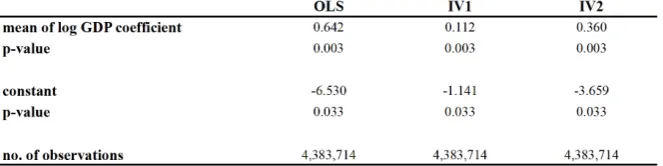
As a further robustness exercise, we test the relationship between quality and income following a two stage approach. First, we estimate quality without considering the income term y in

(11), in line with the original Khandelwal (2010) speci…cation. Then, we assess the relationship between importer income and quality estimates by OLS regression. Table 5 summarizes the results that we obtain on aggregate.23 _{Once again, these results show that the relationship}

between product quality and importer’s income per capita is positive and highly signi…cant.

4

Conclusion

This paper provides theoretical support and empirical evidence on one of the major issues in the international trade literature: whether willingness to pay for quality rises systematically with importer income. Our framework builds on the discrete choice models approach. The novelty of this paper lies in the joint consideration of two features. First, valuation for quality is income dependent and, in particular, their relationship is positive. Second, we depart from the traditional assumption that prices are proxies for quality, and we estimate quality using not only information from prices but also from market shares. We show that a theoretical relationship between these quality measures and consumer income is validated empirically, and discuss under which conditions in terms of income levels and distribution.

2 3_{Tables 9 and 10 in the Appendix respectively report the price and nest coe¢ cients of the …rst-stage estimation}

We bring our predictions to the data, testing our hypothesis on a dataset consisting of import data of …ve EU countries (namely: France, Germany, Italy, Spain and the UK), and over a 13-year time span, i.e., 1995-2007. We …nd a positive and signi…cant relationship between the quality measure and the GDP per capita of the selected countries. Our estimates are robust to a number of controls and to three di¤erent methodological approaches, based on di¤erent instrumental variable strategies.

Appendices

A

Proof of theoretical results

A.1

Derivation of aggregate demand (2)

Consider the choice of a generic good(j; X)over all possible alternatives in the market, namely

f(k; Y)_g, with k₆= j whenY =X. Given (1), the decision rule for consumer i in country M

is as follows: consume good (j; X)only if V_j;Xi;M > V_k;Yi;M,₈(k; Y)₆= (j; X). Our task is thus to compute the probability:

Pr (j; X_ji; M) = Pr "i;M_j;X > max

Y=fN;S;Mg maxj

n

M k;Y +"

i;M k;Y

M j;X

o

(k;Y)6=(j;X)

!

The term on the right-hand side represents the joint probability that horizontal di¤erentiation of good(j; X)is valued by consumeriin countryM more than that of any other good. We can therefore write:

Pr (j; X_ji; M) =

Z +1

1

f "i;M_j;X exp Z

k6=j

ln

Z "i;M_j;X+ M j;X Mk;X

1

f "i;M_k;X d"i;M_k;X

!

dk

+ X

Y6=X

Z 1

0 ln

Z "i;Mj;X+ M j;X

M k;Y

1

f "i;M_k;Y d"i;M_k;Y

!

dk

1

where, exploiting the properties of the exponential function, we have expressed the product of a generic sequencezh as:

Y

h zh=

Y

h

exp (ln (zh)) = exp

X

h

(ln (zh))

The term R"

i;M j;X+ M j;X M k;Y

1 f "

i;M k;Y d"

i;M

k;Y is the cumulative distribution function (CDF) of "i;M_k;Y up to the value"i;M_j;X + M_j;X M_k;Y. Since"i;M_k;Y is a Gumbel random variable, we have:

Z "i;M_j;X+ M j;X Mk;Y

1

f "i;M_k;Y d"i;M_k;Y = Pr "i;M_k;Y < "i;M_j;X + M_j;X M_k;Y

= exp exp h"i;M_j;X + M_j;X M_k;Yi

Replacing this value into (12) yields:

Pr (j; X_ji; M) = Z +1

1

f "i;M_j;X exp Z

k6=j

exp h"i;M_j;X + M_j;X M_k;Xi dk

X

Y6=X

Z 1

0

exp h"i;M_j;X + M_j;X M_k;Yi dk

1

Ad"i;M_j;X (13)

Also, the probability density function (PDF) of a Gumbel random variable is:

f "i;M_j;X = exp "i;M_j;X exp "i;M_j;X

Plugging this expression into (13), and rearranging, we obtain:

Pr (j; X_ji; M) =

Z +1

1

exp "i;M_j;X exp "i;M_j;X 1 + Z

k6=j

exp M_k;X M_j;X dk

+ X

Y6=X

Z 1

0

exp M_k;Y M_j;X dk d"i;M_j;X

=

Z +1

1

exp "i;M_j;X exp "i;M_j;X

X

Y=fN;S;Mg

Z 1

0

exp Mk;Y Mj;X dk d"i;Mj;X (14)

Denote:

$ X

Y=fN;S;Mg

Z 1

0

exp M_k;Y M_j;X dk

and:

g "i;M_j;X exp "i;M_j;X $exp "i;M_j;X

Note thatg "i;M_j;X is the PDF of a Gumbel random variable with CDF:

exp $exp "i;M_j;X =$

since:

dexp $exp "i;M_j;X =$

d" =

exp $exp "i;M_j;X

$ $exp "

i;M j;X

= exp "i;M_j;X $exp "i;M_j;X =g "i;M_j;X

Thus, we can use the last equation to rewrite (14) as:

Pr (j; X_ji; M) = _P 1

Y=fN;S;Mg

R1 0 exp

M

k;Y Mj;X dk

2 4exp

0

@ exp "i;M_j;X X Y=fN;S;Mg

Z 1

0

exp M_k;Y M_j;X dk

1 A 3 5 +1 1

where the term in square brackets vanishes since its limit value for"i;M_{j;X !}+₁equals one, and for"i;M_{j;X ! 1}equals zero. Finally, we multiply and divide byexp M_j;X to get:

Pr (j; X_ji; M) =

exp Mj;X

P

Y=fN;S;Mg

R1 0 exp

M

k;Y dj

A.2

Derivation of optimality conditions (4)-(6)

Di¤erentiating (3) with respect top, and setting the resulting expression equal to zero, yields:

1 pM_j;X wX q2 2AX

Mexp

M

q pM

j;X

P

Y=fM;N;Sg

R1 0 exp

M

k;Y dk

= 0

simplifying and rearranging, (4) straightforwardly obtains. Di¤erentiating (3) with respect toq, and setting the resulting expression equal to zero, we get:

"

qM j;X AX

+ M p wX qM

j;X

2

2AX

!#

Mexp Mqj;XM p

P

Y=fM;N;Sg

R1 0 exp

M

k;Y dk

= 0

Simplifying this expression returns:

qM j;X AX

= M p wX qM

j;X

2

2AX

!

Using (4) to substitute for p = pM

j;X, simplifying and rearranging leads immediately to (5).

Finally, plugging (4) into the de…nition of M_j;X, we have:

M

j;X =qMj;X M

2AX

qj;XM 1 wX

Then, using (5) to substitute forqM

References

[1] Alessandria, G. and Kaboski, J. P. (2011). ‘Pricing-to-Market and the Failure of Absolute PPP,’ American Economic Journal: Macroeconomics, vol. 3, pp. 91-127.

[2] Bastos, P. and Silva, J. (2010). ‘The Quality of a Firm’s Exports: Where you export to matters’, Journal of International Economics, vol. 82, pp. 99-111.

[3] Berry, S. (1994). ‘Estimating Discrete-Choice Models of Product Di¤erentiation’, The RAND Jour-nal of Economics, vol. 25, pp. 242-262.

[4] Berry, S., Levinsohn, J. and Pakes, A. (1995). ‘Automobile Prices in Market Equilibrium’, Econo-metrica, vol. 63, pp. 841–890.

[5] Bils, M. and Klenow, P. J. (2001). ‘Quantifying Quality Growth’,American Economic Review, vol. 91, pp. 1006-1030.

[6] Broda, C., and Romalis, J. (2009). ‘The Welfare Implications of Rising Price Dispersion’, Manu-script, Univ. Chicago.

[7] Choi, Y. C., Hummels, D. and Xiang, C. (2009). ‘Explaining Import Quality: The Role of the Income Distribution’,Journal of International Economics, vol. 77, pp. 265-275.

[8] Fajgelbaum, P., Grossman, G. and Helpman, E. (2011). ‘Income Distribution, Product Quality, and International Trade’,Journal of Political Economy, vol. 119, pp. 721-765.

[9] Fieler, A. C. (2011). ‘Quality Di¤erentiation in Trade:Theory and Evidence’, Mimeo, U Penn.

[10] Flach, L. (2014). ‘Quality upgrading and price heterogeneity: Evidence from Brazilian exporters’, Mimeo.

[11] Flam, H. and Helpman, E. (1987). ‘Vertical Product Di¤erentiation and North-South Trade’, Amer-ican Economic Review, vol. 77, pp. 810-822.

[13] Hallak, J. C. (2006). ‘Product Quality and the Direction of Trade’,Journal of International Eco-nomics, vol. 68, pp. 238-265.

[14] Hallak, J. C. and Schott, P. K. (2011). ‘Estimating Cross-Country Di¤erences in Product Quality’, Quarterly Journal of Economics, vol. 126, pp. 417-474.

[15] Hausman, J. (1997). ‘Valuation of New Goods under Perfect and Imperfect Competition’, in The Economics of New Goods, NBER, edited by Bresnahan, T. and Gordon, R, pp. 209-247.

[16] Hummels, D. and Klenow, P.J. (2005). ‘The Variety and Quality of a Nation’s Exports’, American Economic Review, vol. 95, pp. 704-723.

[17] Jaimovich, E. and Merella, V. (2012). ‘Quality Ladders in a Ricardian Model of Trade with Non-homothetic Preferences’,Journal of the European Economic Association, vol. 10, pp. 908-937.

[18] Jaimovich, E. and Merella, V. (2015). ‘Love for Quality, Comparative Advantage, and Trade’, Journal of International Economics, vol. 97, pp. 376-391.

[19] Khandelwal, A. (2010). ‘The long and short (of) quality ladders’,Review of Economic Studies, vol. 77, pp. 1450-76.

[20] Lancaster, K. J. (1966). ‘A New Approach to Consumer Theory’, Journal of Political Economy, vol. 74, pp. 132-157.

[21] McFadden, D. (1973) ‘Conditional Logit Analysis of Qualitative Choice Behavior’, in Frontiers in Econometrics, New York: Academic Press, edited by P. Zarembka, pp. 105-142.

[22] Murphy, K. and Shleifer, A. (1997). ‘Quality and Trade,’Journal of Development Economics, vol. 53, pp. 1-15.

[23] Pula, G. and Santabárbara, D.G. (2012). ‘Is China Climbing up the Quality Ladder? Evidence Based on EU Imports Data’, Bank of Spain Working Paper Series, 1209.

[24] Simonovska, I. (2010). ‘Income di¤erences and prices of tradables’, NBER Working Paper, 16233.

[26] Verboven, F. (1996). ‘International Price Discrimination in the European Car Market’, RAND Journal of Economics, vol. 27, pp. 240–68.