Networks in Con‡ict: Theory and Evidence from the Great War
of Africa
Michael Königy, Dominic Rohnerz, Mathias Thoenigx, Fabrizio Zilibotti{ April 2, 2014
Abstract
Many wars involve complicated webs of alliances and rivalries between multiple actors. Ex-amples include the recent civil wars in Somalia, Uganda, and the Democratic Republic of Congo. We study from a theoretical and empirical perspective how the network of military alliances and rivalries a¤ects the overall con‡ict intensity, destruction and death toll. The theoretical analysis combines insights from network theory and from the politico-economic theory of con‡ict. We construct a non-cooperative model of tactical …ghting featuring two novel externalities: each group’s strength is augmented by the …ghting e¤ort of its allied, and weakened by the …ghting e¤ort of its rivals. We achieve a closed form characterization of the Nash equilibrium of the …ghting game, and of how the network structure a¤ects individual and total …ghting e¤orts. We then perform an empirical analysis using data for the Second Congo (DRC) War, a con‡ict involving many groups and a complex network of alliances and rivalries. We obtain structural estimates of the …ghting externalities, and use them to infer the extent to which the removal of each group involved in the con‡ict would reduce the con‡ict intensity.
1
Introduction
Alliances and enmities among armed actors play a key role in warfare. In many instances, especially in civil con‡icts, these are not even sanctioned by formal treaties or war declarations, but remain informal and loose relationships. The commands of allied forces are often decentralized and only engage in a limited extent of coordination. More generally, allied groups typically pursue separate goals and compete one with another for the same resource pool over which they …ght common enemies. It is not rare that even open …ghts between belligerent groups that are supposed to be on the same side erupt.
An example of a lose alliance in the context of international wars is the alliance between the Soviet Union and the Anglo-Americans to bring down Nazi Germany during World War II. While sanctioned by international treaties, this was little more than a tactical alliance to defeat a common
PRELIMINARY AND INCOMPLETE DRAFT. We would like to thank André Python, Sebastian Ottinger and Nathan Zorzi for excellent research assistance. We are grateful for helpful comments by Alessandra Casella, Andrea Ichino, Macartan Humphreys, Massimo Morelli, Uwe Sunde, Giulio Zanella, and conference and seminar participants in the universities of Bologna, CERGE-EI, Columbia, , European University Institute in Florence, IMT Lucca, INSEAD, Luxembourg, Marseille-Aix, Nottingham, Munich, Pompeu Fabra, SAET Paris, Southampton, St. Gallen, Toulouse, Zurich.
enemy. Well before the war was over, the Soviet Union and the Anglo-Americans were …ghting strategically for con‡icting objectives, each trying to secure the best political and military outcome at the end of the con‡ict. This goal informed their choice of military targets (e.g., the Red Army did not intervene in support of the Warsaw insurrection regarding it as a hostile attempt orchestrated by London to gain control over Poland; Stalin geared its military campaign to reach Berlin before the allied forces; etc.) and the investments of human and physical resources in the con‡ict. Similar considerations apply to earlier wars, from the Peloponnesian War in the ancient Greece, to the Napoleonic Wars (cf. for example Ke et al, 2013), or to the alliances between warlords in China after the proclamation of the Republic in 1912. The recent civil con‡icts in Afghanistan, …rst at the time of the Soviet occupation, and after the NATO intervention in 2001, were instances in which informal alliances and enmities played an important role (see Bloch, 2012). The same is true for many civil wars in Africa, including Somalia, Uganda, Sudan or the Democratic Republic of Congo. In this paper, we construct a theory of con‡ict focusing explicitly on the role of the network of alliances and enmities. The maintained assumption is that each group involved in the con‡ict maximizes its individual pay-o¤ given by the share of resources controlled at the end of the con‡ict (the "prize") net of the resources sank in the battle…eld. The equilibrium is determined as the standard Nash equilibrium of a non-cooperative game. The benchmark is acontest success function, henceforth CSF (see, e.g., Hirshleifer 1989; Skaperdas, 1992; Grossman and Kim, 1995). In a standard CSF, the share of the prize accruing to each group is determined by the relative amount of resources (…ghting e¤ ort) that each of them commits to the con‡ict. In our model, the network of alliances and enmities introduces additional externalities. More precisely, the share of the prize accruing to each group hinges on its relative strength, that we label asoperational performance. In turn, this is determined by its own …ghting e¤ort augmented by the …ghting e¤ort of all allied groups (weighted by an allied externality parameter) and diminished by the …ghting e¤ort of all enemy groups (weighted by an enemy externality parameter). Thus, when a group increases its …ghting e¤ort, it also a¤ects, positively, the operational performance of its allied groups, and negatively that of its enemy groups.1 The complex externality web a¤ects the optimal …ghting e¤ort of all groups. Enemy relationships induce strategic complementarity in …ghting e¤orts, whereas alliances induce strategic substitution.
We provide a full analytical solution for the Nash equilibrium of the game. Absent other sources of heterogeneity, the …ghting e¤ort of each agent is pinned down by its centrality in the network. Our novel centrality measure is related to the Bonacich centrality (see Ballester, Calvo-Armengol and Zenou, 2006). More precisely, it is approximately equal to the sum of the Bonacich centrality related to the network of hostilities, and the (negative-parameter) Bonacich centrality related to the network of alliances. The share of the prize accruing to each player has a particularly simple solution: it can be expressed as the ratio between a simple function of the …rst-degree links (i.e., the number of direct allied and enemies a group has) –a measure that we labellocal hostility level – and the sum of the total hostility levels of all agents involved in the con‡ict. Interestingly, the more allies a group has, the smaller the share of the prize it appropriates – although the same result need not apply to the set of allies taken together. In contrast, welfare (i.e., the share of the prize net of the …ghting e¤ort) is increasing in the number of allies and decreasing in the number of enemies. Intuitively, alliances su¤er from a free riding problem. Consider, for instance, a con‡ict involving three groups, two of them being allied against the third group. When each member of the alliance exerts costly e¤ort, part of its e¤ects spills over to the allied group. Hence, the marginal bene…t of …ghting is smaller for each of the two allies than for the isolated group.
Together with determining the …ghting e¤ort and success of each individual player, the network
of alliances and hostilities determines the size of the con‡icts, or the total rent dissipation, which is the inverse measure of aggregate welfare. In general, the abundance of hostility links lead to more rent dissipation, while the opposite is true for alliances. This is well illustrated in regular graphs, in which the number of alliances and enmities is invariant across groups. The con‡ict escalation (and rent dissipation) is maximum when all groups are enemy of each other (as in Hobbes’homo homini lupus), whereas it is minimized in networks where all groups are in friendly terms (as in Rousseau’s well-order society). The well-order society is a somewhat surprising outcome, as it results from a sel…sh behavior in a non-cooperative contest. The reason is that the marginal product of …ghting e¤ort becomes small when all agents are allied and the alliance externality is su¢ ciently small. Free riding is socially desirable, since war e¤ort has no social value. This peaceful outcome can be viewed as a paradigmatic representation of societies in which the system of institutional check and balances reduces the incentive for opportunistic behavior.
In the second part of the paper, we perform an empirical analysis based on the structural equations of the model. We focus on the Second Congo War, which is also sometimes referred to as the "Great African War" and whose estimated death toll ranges between 3 and 5 million lives (Olsson and Fors, 2004; Autesserre, 2008). More details about the historical context of the con‡ict are provided in Section 3.1. This con‡ict involves a large number of groups, and a rich network of alliances and enmities. We use information from Armed Con‡ict Location Event Database (ACLED) and the Stockholm International Peace Research Institute (SIPRI) to identify the network of alliances and enmities. We assume that the network is constant over time (an assumption that conforms with the data, at least for the period we consider) and proxy …ghting e¤ort by the annual observations for the number of …ghting events in which each group is involved. The estimation uses the panel of annual observations controlling for group …xed e¤ects and time-varying observed heterogeneity. In particular, we focus on weather shocks, that have been shown in the previous literature to have important e¤ects on …ghting intensity (cf. e.g. Miguel et al. 2004, Vanden Eynde 2011, and Rogall 2013). Weather shocks are especially important in our analysis, as they provide the exogenous source of variation that allows us to achieve identi…cation, following the methodology proposed by Bramoullé et al. 2009 (see also Liu et al. 2011). In particular, our identi…cation exploits the exogenous variation in the average weather conditions facing, respectively, the set of allies and of enemies of each group. Without imposing any restriction on the estimation procedure, we …nd that the two estimated externalities have the signs predicted by theory.
After estimating the model, and in particular gauging the size of the network externalities, we can calculate how important each player is in the determining the total intensity of the con‡icts. More formally, we perform a key player analysis, i.e., we ask how the total rent dissipation would change if each of the player were individually removed, and all other players were to readjust their …ghting e¤ort. We view this as a policy-relevant exercise, as it allows international organizations (e.g., the UN) to identify the actors whose decommissioning would be most e¤ective to scale down con‡ict. Interestingly, while on average large groups are more crucial than small ones, the relation-ship is not one-to-one. The hypothetical removal of some relatively small players such as the Lord Resistance Army turns out to have large e¤ects on the containment of the DRC con‡ict. Intuitively, the war activity of the LRA increases the military operations of its traditional enemy, the armed forces of Uganda. This, in turns, spills over to the activity of the DRC army and its allied, that are enemies of the Ugandan army for di¤erent reasons.
choose their …ghting e¤orts to attack their neighbors. However, di¤erently to the current paper, they do not allow for alliances. Moreover, they can only characterize equilibrium e¤orts for very speci…c networks (regular, star-shaped, and complete bipartite graphs). In contrast, we provide an equilibrium characterization for any network structure. This allows us to apply our model to the data, and to perform a key player analysis. Hiller (2012) studies the formation of networks where agents can form alliances to coerce payo¤s from enemies with fewer friends. However, the payo¤ structure is rather speci…c, and, more importantly, it does not allow for endogenous choice of …ghting e¤orts in con‡ict. Moreover, none of the above papers is applied to data, and neither do they provide a structural estimation of the model’s parameters which is necessary for our key player analysis. A notable exception is the recent paper by Acemoglu, Garcia-Jimeno and Robinson (2014) that estimates a structural model of political economy of public goods provision using a network of Colombian municipalities. However their object of inquiry is very di¤erent as they are interested in estimating the spillover e¤ects of local state capacity across municipalities.
The problem of identifying key players in strategic games on networks is pioneered by Ballester et al. (2006). The authors determine equilibrium e¤ort choices in a game of strategic complements between neighboring nodes, and identify key players, i.e. the agents whose removal reduces equi-librium aggregate e¤ort the most. However, their payo¤ structure is substantially di¤erent from ours, and does not incorporate an environment in which agents are competing in a contest over common resources. More recently, the key player policy has also been tested empirically. Liu et al. (2011) test the key player policy for juvenile crime in the United States, while Lindquist and Zenou (2013) identify key players for co-o¤ending networks in Sweden. Di¤erently to these works we analyze key players in armed con‡icts, and provide an application to the war in Congo.
Further, our study is also related to the growing politico-economic con‡ict literature.2 Papers in this literature typically focus on settings with two large groups facing each other, and they do not consider network relationships. A few papers consider multiple groups comprising each a large number of players, and study collective action problems. Esteban and Ray (2001) show that the Olson paradox does not generally hold and that sometimes large groups can be more e¤ective than small groups. To this purpose they build a model with n di¤erent groups composed each of a varying number of individual players. Individual players select costly …ghting e¤ort and the winning chances of each collective group depends on its total e¤ort as a share of the sum of all group e¤orts in society. Their model is di¤erent and complementary to ours, since it does not consider general network structures, but focuses on a setting comprising n di¤erent cliques, where there are no links between cliques.3
There is also a small numbers of papers that study explicitly the role of alliances in settings with either three players, or identical players (cf. Konrad, 2009, 2011, and Bloch, 2012 for surveys). Some papers note, as we do, that alliances may be socially desirable since they reduce rent dissipation in wars (cf. Olson and Zeckhauser 1966, Wärneryd 1998, and Gar…nkel 2004). In this context, a few papers regard the mere existence of alliances as a "puzzle" given the problem they generate (cf. Nitzan 1991, Skaperdas 1998, Esteban and Sakovics 2004, Sanchez-Pagés 2007, Konrad and Kovenock 2009). These papers emphasize that (i) there is a collective action problem within the alliance, leading to free-riding, and hence lower aggregate e¤ort; (ii) after being successful there
2Recent work in this …eld links con‡ict to state capacity (Besley and Persson, 2011), trust and social capital (Rohner, Thoenig and Zilibotti, 2013, Acemoglu and Wolitzky, 2014), trade (Martin et al. 2008; Dal Bo and Dal Bo, 2011), political bias and institutions (Jackson and Morelli, 2007; Conconi, Sahuguet, and Zanardi, 2014), natural resource abundance and inequality (Caselli et al., 2013; Morelli and Rohner, 2014), and the e¤ects of ethnic diversity (Esteban and Ray, 2008; Caselli and Coleman, 2013).
3
may be a second stage with con‡ict within the victorious alliance, which further reduces incentives for …ghting e¤ort in the …rst stage of the game. To address the puzzle, Konrad and Kovenock (2009) argue that capacity constraints can explain the establishment of alliance, while Skaperdas (1998) argues that alliances can only form when the CSF has increasing returns characteristics. This literature focuses either on settings with only three players, or alternatively on frameworks with n identical and symmetric players. In contrast, our analysis focuses on complex networks where the di¤erent centrality of di¤erent players play a decisive role. We take the web of alliances as given and do not try to rationalize them.
Our paper is also embedded in the empirical literature on civil war (cf. e.g. Fearon and Laitin, 2003; Collier and Hoe- er, 2004), and in particular in the recent literature that studies con‡ict using very disaggregated micro-data on geo-localised …ghting events, such as for example Dube and Vargas (2013), Cassar, Grosjean, and Whitt (2013), Michalopoulos and Papaioannou (2013), Rohner, Thoenig, and Zilibotti (2013b), and La Ferrara and Harari (2012).
The paper is organized as follows: Section 2 presents the theoretical model, the equilibrium and the welfare analysis; Section 3 discusses the application to the Second Congo War; Section 4 concludes.
2
The Model
2.1 Environment
The model economy is populated by a network of n agents (groups), G 2 Gn, where Gn denotes the class of graphs onnnodes. Each pair of agents can be in one of three bilateral states: alliance, hostility, or neutrality. We represent the set of bilateral states by the matrixA= [aij]1 i;j nwhere
aij 2 f 1;0;1g. More formally, A is the signed adjacency matrix associated with the network G
(cf. Zaslavsky 1982), where:
aij = 8 > < > :
1; ifiand j are allied; 1; ifiand j are enemies;
0; ifiand j are in a neutral relationship:
Note that a neutral relationship is modelled as the absence of links. IfA does not contain any zero entries, we say that we have complete signed network.
Let a+ij maxfaij;0g and aij minfaij;0g denote the positive and negative parts of aij,
respectively. Then, aij = a+ij aij, respectively, for all 1 i; j n. Similarly, A = A++A
where A+ =haiji
1 i;j n and A = h
aiji
1 i;j n. We denote the corresponding subgraphs as G +
and G , respectively, so thatGcan be written as the graph joinG=G+ G . Finally, we de…ne by d+i Pnj=1a+ij agent i’s number of alliances, and bydi Pnj=1aij his number of enmities.
The n agents compete for a prize whose total value is denoted byV >0. We assume agents’ payo¤s to be determined by a CSF. The CSF maps the relative …ghting intensity each agent devotes to a con‡ict into the share of the prize he appropriates after the con‡ict. More formally, we postulate a payo¤ function i:Gn Rn+ !Rsuch that
i(G;x) =
'i(G;x) Pn
j=1'j(G;x)
V xi; (1)
on agent i’s own …ghting e¤ort, as well as on his allied’s and enemies’s e¤orts. More formally, we assume that
'i(G;x) xi+ n X
j=1 a+ijxj
n X
j=1
aijxj; ; 2[0;1]: (2)
Note that the speci…cation of Equation (2) assumes no heterogeneity across agents other than their position (i.e., the number of allies and enemies) in the network. We will introduce heterogeneity in Section 2.5 below.
Equation (2) is our main theoretical assumption. It postulates that each agent’s OP increases in the total e¤ort exerted by the allied and decreases in the total e¤ort exerted by the enemies. These externalities compound with those embedded in the pay-o¤ of the standard CSF, which equation (2) nests as the particular case in which a+ij = aij = 0 for all i and j: In this case,
i = xi=Pnj=1xj V xi, and each agent’s e¤ort imposes a negative externality on all other
agents in the contest only by increasing the denominator of the CSF. Consider, next, a case in which a+ij > 0 and > 0; for one and only one pair (i; j) (while aij = 0 for all i and j). Then,
i = (xi+ xj)=Pnj=1xj V xi: In this case, an increase in agent j0s e¤ort entails both the
standard negative externality through the denominator, and, in addition, the positive externality captured by an increase in the numerator. Thus, holding e¤orts constant, a newly established alliance between i and j increases the share of V accruing jointly to i and j, at the expenses of the remaining groups. To, the opposite hostility links strengthen the negative externality of the standard CSF. For instance, suppose thatn= 3and that all agents exert the same …ghting e¤ort,
x1 = x2 = x3 = x: Then, the standard CSF prescribes an equal division of the pie. However, if
agents1 and2 are enemies, while agent 3 is in a neutral relationship with both, then agents1 and
2earn a smaller share of the pie each, while agent earn a larger share of it. For instance, if = 1=2, agents 1and 2 receive a quarter of the pie each, while agent3 appropriates half of it.
2.2 Equilibrium Fighting E¤ort
In this section, we endogenize the …ghting e¤ort choice, and characterize the Nash equilibrium of the contest. More formally, each agent chooses e¤ort (xi) non-cooperatively in order to maximize i(G;x), given all other agents’e¤orts,x i. We impose no restrict to the e¤ort choice, and allow,
in principle, negative e¤ort choices.4 The First Order Conditions yield, for all i= 1;2; : : : ; n:
@ i(G;x) @xi
= 0()'i= 1 1 + d+i di
0 @1 1
V n X
j=1 'j
1 A
n X
j=1 'j;
where we assume that, for all i; d+i di > 1:5 Solving the system of n equations yields the equilibrium OP levels:
'i (G) = ; (G) 1 ; (G) i; (G) V; (3)
where
; i (G)
1
1 + d+i di and
; (G) 1 1
Pn i=1
; i (G)
: (4)
4
Formally, the zero e¤ort level is purely a matter of normalization. One could as well rewrite the model by replace
xiwith(x xi);where(x xi)denotes the e¤ort level. All results would be unchanged. More importantly, we rule
out a participation decisions. Agents have no option to stay out of the con‡ict (e.g., because they would be subject to expropriation of their endowments).
5
Summing over iyields the total economy-wide OP level,
n X
i=1
'i = ; (G) V; (5)
which in turn implies that
'i Pn
j=1'j =
; i (G) Pn
j=1 ; j (G)
(6)
;
i is a measure of local hostility level capturing the externalities associated with agent i’s
…rst-degree alliance and hostility links. ; is a measure oftotal OP in the network. Both i; (G) and
; (G) are decreasing with , and increasing with . Equation (5) implies that the total OP is
decreasing in the number of bilateral alliances and in ;and increasing in the number of hostility links and in . Moreover, equations (1) and (6) show that the share of the prize accruing to each agent in equilibrium increases in the number of direct alliances and decreases in the number of enmities.
Next, we characterize agents’equilibrium …ghting e¤orts, and how these depend on the struc-ture of the network. The following Proposition provides a complete characterization of the Nash equilibrium:
Proposition 1 Assume that + <1=maxf max(G+); dmaxg and max(A+)<1 max(A );
where max(A ) denotes the largest eigenvalue associated with the matrix A . Let i; (G) and
; (G) be de…ned as in (4), and let
c ; (G) In+ A+ A 1 ; (G) (7)
be a centrality vector, whose generic element ci; (G) describes the centrality of agent i in the network. Then, there exists a unique Nash equilibrium with e¤ ort levels given by
xi (G) = ; (G) 1 ; (G) ci; (G) V; (8)
for all i= 1; : : : ; n. Moreover, the equilibrium OP levels are given by (5), and the payo¤ s are given by
i(G) = i(x ; G) =V(1 ; (G)) i; (G)
; (G)c ;
i (G) : (9)
The centrality measure,ci; (G);plays a key role in Proposition 1. Note, in particular, that the relative …ghting e¤orts of any two agents only depends on their relative centrality in the network:
xi(G) xj(G) =
ci; (G) cj; (G):
Whileci; (G)depends in general on the links of all degrees, it is enlightening to focus on the case in which the spillover parameters and are small. In this case, our centrality measure can be approximated by the the sum of (i) the Bonacich centrality related to the network of hostilities,
G , (ii) the (negative-parameter) Bonacich centrality related to the network of alliances, G+, and (iii) the local hostility vector, ; (G) (cf. Ballester et al., 2006; Liu et al., 2011).6
Corollary 1 As ! 0 and !0; the centrality measure de…ned in Equation (7) can be written as
c ; (G) =b ; (G)( ; G ) +b ; (G)( ; G+) + ; (G) +O( );
where O( ) involves second and higher order terms, and the ( -weighted) Bonacich centrality
with parameter is de…ned as
b ( ; G)
1 X
k=1
kAk ; (10)
as long as the invertibility condition j j<1= max(G) is satis…ed.
Corollary 1 states that the centrality c ; (G) can be expressed as a linear combination of the weighted Bonacich centralitiesb ; (G)( ; G )andb ; (G)( ; G+)plus the vector ; (G). Each
Bonacich centrality gauges the network multiplier e¤ect attached to the system of hostilities and alliances, respectively. In particular, b ; (G)( ; G ) captures how a groupiis in‡uenced by all its
(direct and indirect) enemies.7 In the case of small ; b ; (G)( ; G ) can be itself approximated
as follows (ignoring terms of degree three or higher):
b ; (G);i ; G = i; (G) +
n X
j=1
aij j; (G) + 2 n X
j=1 aij
n X
k=1
ajk k; (G) +O 3 :
Similarly,
b ; (G);i( ; G+) = i; (G) + ( )
n X
j=1
a+ij j; (G) + ( )2 n X
j=1 a+ij
n X
k=1
a+jk k; (G) +O 3 :
Thus, Corollary 1 suggests that, when higher degree terms can be neglected, our centrality measure is increasing in and in the number of degree-one and degree-two enmities, whereas it is decreasing in and in the number of degree-one alliances. Degree-two alliances have instead a positive e¤ect on the centrality measure.8
In the case of weak network externalities (i.e., ! 0 and ! 0; as above) we can as well obtain simple approximate expression for the equilibrium e¤orts and the payo¤s in Proposition 1.9
Corollary 2 As ! 0 and !0; the equilibrium e¤ ort and payo¤ of agent iin network G can be written as
xi(G) = Xo(G; ; ; n) +X1(G; ; ; n) di d +
i V +O( )
i(G) = o(G; ; ; n) + 1(G; ; ; n) d+i di V +O( )
where X0; X1; 0; 1 are unimportant positive constants (see the proof of Corollary 2 in Appendix
A).
7
The Bonacich centrality measure related to the network of hostilities, b ; (G);i ; G , measures as the local
hostility levels along all walks reachingiusing only hostility connections, where walks of length kare weighted by the geometrically decaying hostility externality k. Due to the approximation, we only consider links up to degree
two.
8The intuition for this last, perhaps surprising, property is related to the relationship of complementarity and substitution among …ghting e¤orts, as will become clear below. To anticipate the argument: Ifiis allied with jand
jis allied withk;an increase in the …ghting e¤ort ofkreduces the …ghting e¤ort ofjand this, in turn, increases the …ghting e¤ort ofi:Consider, instead, the case in whichiis enemy tojandjis enemy tok:Then, an increase in the …ghting e¤ort ofkincreases the …ghting e¤ort ofjand this, in turn, increases the …ghting e¤ort ofi:
9
It is also useful to note that, when = = 0;then ; = 1 n1;and ci; = ;
i = 1:Then, the equilibrium
expressions in Proposition 1 simplify toxi =V(n 1)=n2 and i =V =n2which is are the standard solutions in the
Figure 1: The …gure shows an example of a line graphL5 with …ve agents.
Corollary 2 shows that, when network externalities are small, an agent’s …ghting e¤ort increases in the weighted di¤erence between the number of enmities (weighted by ) and of alliances (weighted by ). The opposite is true for the equilibrium pay-o¤, that is increasing in d+i di . Thus, ceteris paribus, an increase in the spillover from alliances (enmities), parameterized by ( ), as well as an increase in the number of allied (enemies) decreases (increases) agent i’s …ghting e¤ort and increases (reduces) its pay-o¤. Intuitively, an agent with many enemies tends to …ght harder and to appropriate a smaller share of the prize, whereas an agent with many friends tends to …ght less and to appropriate a large size of the pie. One must remember that this simple result may be reversed if higher-degree links have sizable e¤ects.
2.3 Example: a line graph
In this section, we consider the illustrative example of a line graphL5 with …ve agents, as depicted
in Figure 1. This example highlights the role of the centrality of di¤erent players.
Suppose, …rst, that >0, and all links in Figure 1 are enmities. If two agents are not linked, they are in neutral terms. Thus, agent1 is an enemy of agents2and 4, while agent 3 is an enemy of agent 2 and agent5 is an enemy of agent4. Because of pair-wise symmetry, equilibrium e¤orts and payo¤s for agents 5 and 3as well as for 4and 2 are identical. The ranking of the e¤ort level, for any ;features:10
x1 > x2=x4> x3 =x5:
Agent1 always exerts a higher e¤ort than agent 2, because agent1 is more central in the network and thus experiences a higher network multiplier e¤ect. This consistent with the result that e¤ort levels are proportional to the Bonacich centrality (cf. Corollary 1). Conversely, the equilibrium payo¤ of agent 1 is smaller than the payo¤ of agent 2. Moreover, equilibrium e¤ort of agent 3 is lowest, and the payo¤ is highest as this agent is the least central in the network and thus experiences the least network multiplier e¤ect from con‡icts. The upper left and upper right panel of Figure 2 show, respectively, e¤ort levels and pay-o¤ for varying values of . Fighting e¤ort and payo¤s are increasing and decreasing in ;respectively.
Consider, next the polar opposite case in which >0, and all links in Figure 1 are alliances. If two agents are not linked, they are in neutral terms, as before. The following equilibrium …ghting
1 0The analytical expressions yield:
x1=V
2( ( + 2) 2) 3 2+ 1 1 (5 7 )2(3 2 1)
x2=x4 =V
2 ( (3 + 5) 9) 2+ 2 (5 7 )2(1 3 2)
x3=x5 =V
e¤ort ranking results:11
x2 =x4< x1< x3 =x5:
The lower left and right panels of Figure 2 show, respectively, e¤ort levels and payo¤s for di¤erent values of . We observe that, for a low range of ’s, the least central agents, 3 and 5, exert the highest …ghting e¤ort and earn the lowest payo¤. However, for higher ’s, agents 3 and 5 earn a higher pay-o¤ than agent 1. It is interesting to note, in addition, that it is agents 2 and 4 who exert lowest e¤ort, in spite of agent 1 being the most central player. The reason is that agents 2
and 4 are connected, respectively, to agents 3 and 5 who lie at the periphery of the network, and have no other connections. Thus, agents 3 and 5 exercise very high e¤ort, and this is exploited by agents 2 and 4, who can reduce their …ghting e¤ort and earn a higher payo¤.12 Finally, the non-monotonicity of e¤orts and payo¤s for agents1 and3(and5) is related to the fact that, when is high, agent2 (and4) reduces a lot its …ghting e¤ort, inducing substitution (i.e., higher e¤ort) from the neighbor. Interestingly, for very high ;this e¤ect is stronger for agent 1 than for agent
3;so the most central agent ends up earning the lowest pay-o¤ among all agents in the contest. Note that in both cases (upper and lower panels in Figure 2) the results are consistent with Corollary 2, which requires externalities to be small. In the upper panel, as ! 0 the e¤ort is higher and pay-o¤ is lower for the agents who have two enemies (i.e., agents 1;2 and 4) than for the agent in the periphery (agents 3and 5) who have only one enemy. In this case, this is true for any :In the lower panel, as !0the e¤ort is lower and pay-o¤ is higher for the agents who have two allies (i.e., agents1;2 and 4) than for the agents with only one ally (agents 3 and 5). In this case, however, the result changes as one takes larger ’s, as discussed above.
2.4 Welfare Analysis
In this section, we discuss welfare and policy implications of the theory. Our (negative) welfare measure is the extent of rent dissipation, which is equal to the total equilibrium …ghting e¤ort as a share of the prize of the context. This is given by:
RD ; (G) 1 V
n X
i=1
xi(G) = ; (G)(1 ; (G)) n X
i=1
ci; (G):
Since the aggregate welfare isPni=1 i(G) =V 1 RD ; (G) ; then, minimizing rent dissipation is equivalent to maximizing welfare.
2.4.1 E¢ cient Networks
We start by analyzing how the network structure a¤ects rent dissipation. Intuitively, one might expect that abundant alliances tend to reduce rent dissipation, by decreasing the marginal return
1 1The analytical expressions are:
x1=V
2 2( + 1)( (3 10) + 5) 2 (7 + 5)2 3 2 1
x2=V
2 2( (5 3 ) + 9) 2
(7 + 5)2 3 2 1
x3=V
2(( 2) 2)( ( + 1)(3 1) 1)
(7 + 5)2 1 3 2 :
1 2
Figure 2: The …gure shows the equilibrium e¤orts (left panels) and payo¤s (right panels) as functions of and for two line graphs in which there are only hostile relationships (upper panels) and only alliances (lower panels), respectively.
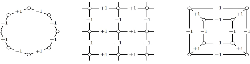
of individual …ghting e¤ort, the opposite being true for enmities. While this becomes complicated in general networks, a simple proof can be provided for the particular case of regular graphs, i.e., networks in which every agent i has d+i =k+ alliances and di = k enmities. An illustration is shown in Figure 3.
We denote a regular graph by Gk+;k . The Nash equilibrium is in this case symmetric: all agents exercise the same e¤ort, and 'i =' = 1=n, implying an equal division of the pie. Under the conditions of Proposition 1,13 the equilibrium e¤ort and payo¤ are given by, respectively,
xi Gk+;k =x k+; k =
1 1 + k+ k
1 n
V
n; (11)
i Gk+;k = k+; k =
1 + (1 +n)( k+ k ) n(1 + k+ k )
V
n: (12)
Standard di¤erentiation implies that
@x (k+; k ) @k+ <0;
@x (k+; k ) @k+ >0;
@ (k+; k ) @k >0;
@ (k+; k ) @k <0:
Intuitively, …ghting e¤ort and rent dissipation increase (decrease) in the number of enmities (al-liances). The regular graph nests three interesting particular cases. First, if = = 0, we obtain the standard equilibrium of the Tullock game, withRD0;0 Gk+;k = (n 1)=n:Second, consider a complete network of alliances (k+ = n 1), where, in addition, ! 1: Then, x ! 0 and
1 3We require that + <1=max
Figure 3: The …gure shows three examples of regular graphsGk+;k : The left panel shows a regular graph with k+ = k = 1 , the middle panel shows a regular graph with k+ =k = 2 (assuming periodic boundary conditions, i.e. a torus), and the right panel a Cayley graph with k+ = 1 and
k = 2.
Figure 4: The …gure shows the equilibrium e¤orts (left panel) and pay-o¤ (right panel) in the case in which there are no enmities. Parameters: k+ 2 f1;5;10g; V = 1 and n = 100. Equilibrium
e¤orts are decreasing in and k:
RD1; (Gn 1;0) ! 0; i.e., there is no rent dissipation. Namely, the society attains peacefully the
equal split of the surplus, as in Rousseau’s harmonious society. The lack of con‡ict does not stem here from social preferences or cooperation, but from the equilibrium outcome of a non-cooperative game between sel…sh individuals. The crux is the strong …ghting externality across allied agents, which takes the marginal product of individual …ghting e¤ort down to zero. Third, consider, con-versely, a society in which all relationships are hostile, i.e.,k =n 1. Then,RD ; (G0;n 1)!1
as ! 1=(n 1)2: all rents are dissipated through …erce …ghting, as in Hobbes pre-contractual society wherehomo homini lupus est.
Figure 4 shows how the equilibrium e¤ort and payo¤s change as a function ofk+and assuming no enmities (or = 0). Higher and higherk+induce lower e¤ort and higher payo¤s. The reason is that the substitutability e¤ect of allied agents increases with both (strength of the alliances) and
following Proposition.
Proposition 2 Let the e¢ cient graph G 2 Gn be the graph that minimizes the rent dissipation.
Then we have that
0 RD ; (G ) RD ; (Gn 1;0) =
1 1 + (n 1)
1 n;
where Gn 1;0 is the complete graph where all agents are allies. Consequently, when either ! 1
or n! 1;then, RD ; (G )!0;and the e¢ cient graph is G =Gn 1;0.
2.4.2 The Key Player
Thekey playeris de…ned as the agent whose removal triggers the largest reduction in rent dissipation Ballester et al. (2006) Identifying the key player is important to determine which policy intervention can reduce …ghting activity.
De…nition 1 Let G i be the network obtained from G by removing agent i; and assume that the conditions of Proposition 1 hold. Then the key player i 2 N =f1; : : : ; ng [ ; is de…ned by
i = arg max i2N
n
RD ; (G) RD ; G i o; (13)
where RD ; (G) Pni=1xi(G) =V ; (G)(1 ; (G))Pn
i=1c ;
i (G), and xi (G) is the generic
element of the vector x (G) de…ned in Equation (8).
Note that the welfare di¤erence RD ; (G) RD ; G i can be interpreted as the maximum cost a benevolent policy maker would be willing to pay to induce or force agentinot to participate in the contest. Note also that the key player in De…nition 1 might be empty if none of the agents can be removed so that the rent dissipation is reduced.
The identity of the key player is related to the centrality measure de…ned in Equation (7). Consider, for instance, the case is which all agents have the same technology. Then, the de…nition of the key player simpli…es to (see also Proposition 4 in Appendix A)
i = arg max i2N
8 < :
n X
j=1
cj; (G) +X j6=i
hi; (G) (1 1 ; (G) h ; i (G)) 1 ; (G)
n X
k=1 "
mjk; (G) m ; ij (G)m
; ik (G) mii; (G)
! ; k (G)
1 + d+k dk
1 + d+k 1 dk1fk2Ni+g
+ 1 + d + k dk
1 + d+k dk 1 1fk2Ni g+ 1fk =2(N
+
i [Ni )g
!#)
; (14)
where N f1; : : : ; ng [ ;; 1fk2N+
i g and 1fk2Ni g are indicator variables taking the unit value if,
respectively,k2 Ni+and k2 Ni , and zero otherwise, we have de…ned by
hi; (G) = 0
@1 X
j2Ni+
;
j (G) (1 ; (G)) 1 + d+j 1 dj
X
j2Ni
;
j (G)(1 ; (G)) 1 + d+j dj 1
1 A
1
and mij; (G) is theij-th element of the matrixM ; (G) = (In+ A+ A ) 1. It is important
to note that the key player identi…ed in Equation (14) di¤ers signi…cantly from the one introduced in Ballester et al. (2006) , where the key player is de…ned as i = arg maxi2N bNu;ii((G;G; )) with
bu;i(G; ) being the Bonacich centrality of agentiin G(see also Equation (10) and Appendix B),
andNi(G; )counting the number of closed walks starting and ending atiwhere the length of the
walks is discounted by powers of . Our key player formula is more involved due to the non-linearity inherent in the contest success function in the agents’payo¤s.
2.5 Heterogenous Fighting Technologies
So far, we have maintained that all agents have access to the same …ghting technology to turn e¤ort into …ghting intensity. This has allowed us to focus sharply on the network as the only source of heterogeneity. In reality, military groups typically di¤er in size, wealth, access to weapons, etc. In this section we generalize our model by allowing heterogeneous …ghting technologies. We study both additive and multiplicative e¤ects
Suppose, …rst, that agent i’s …ghting strength can be written as
'i = ~'i+xi+ n X
j=1 a+ijxj
n X
j=1
aijxj: (15)
where '~i is an additive shock a¤ecting group i0s OP (e.g., its military capability). The payo¤ function in Equation (1) can then be written as follows:
i(G;x) =V 'i Pn
j=1'j
xi=V
xi+ Pnj=1a+ijxj Pnj=1aijxj + ~'i Pn
j=1 xj + Pnk=1a+jkxk
Pn
k=1ajkxk+ ~'j
xi: (16)
One can show that the equilibrium OP is unchanged, and continues to be given by Equation (3). Likewise, Equation (6) continues to characterize the share of the prize appropriated by each agent. Somewhat surprising, P'i
n
j=1'j is independent of '~i: In contrast, '~i a¤ects the equilibrium e¤ort
exerted by each agent. In particular, the equilibrium …ghting e¤ort vector is now given by (see Proposition 5 in Appendix A)
x = (In+ A+ A ) 1(V ; (G)(1 ; (G)) ; (G) '~); (17)
under the same assumptions and de…nitions of ; and ; (G)given above, and under the addi-tional assumption thatV ; (G)(1 ; (G)) ; (G)>'~. This extension is important, as it will allow us to introduce observable and unobservable sources of heterogeneity into the econometric model below.
Another generalization involves allowing heterogeneity in the productivity of …ghting e¤ort. Suppose for instance that agenti’s …ghting strength can be written as
'i= ixi+ n X
j=1
a+ij jxj n X
j=1
aij jxj; (18)
with i 2R+ is a measure of the individual …ghting technology. The payo¤ function of Equation
(1) can then be written as follows
i(G;x; ) =V 'i Pn
j=1'j
xi=V
ixi+ Pnj=1aij j+ xj Pnj=1aij jxj Pn
j=1 jxj+ Pnk=1a +
jk kxk Pnj=1ajk kxk
where ( 1; : : : ; n)> 2 Rn+. Proposition 1 can then be generalized to the heterogenous case.
The Nash equilibrium is given by (see Proposition 6 in Appendix A)
x (G; ) =V~ ; (G; )D( ) 1(In+ A+ A ) 1(In ~ ; (G; )D( ) 1) ; (G); (20)
where
~ ; (G; ) u> ; (G) 1
u>D( ) 1 ; (G)
is a measure of "local …ghting intensity", D is a diagonal matrix, and u> is a vector of ones. Intuitively, ceteris paribus, a high- agent can a¤ord to exert low e¤ort because each unit of his e¤ort translates into a high …ghting intensity. Consequently, his payo¤ tends to be high. The de…nition of rent dissipation is modi…ed, accordingly: RD ; (G; ) V1 Pni=1(1 + i)xi (G; );
wherexi (G; )is the generic element of the vectorx (G; )de…ned in Equation (20) and >0 a positive constant.
3
Empirical Application - The Second Congo War
In this section, we apply the theoretical model constructed in Section 2 to the study of the recent civil con‡ict in the Democratic Republic of Congo (henceforth, DRC). Our goal is to estimate key externality parameters and from a structural equation such as (15) characterizing the Nash equilibrium of the model. The estimates are used, on the one hand, to test some restrictions imposed by the theory, and, on the other hand, to perform some policy analysis. We start by presenting the historical context of the DRC con‡ict. Then, we discuss the data sources. Next, we discuss how we estimate the network structure from the data. We proceed then to the econometric model and the discussion of identi…cation and estimation procedure. Finally, we discuss some policy analysis (key player analysis).
3.1 Historical Context
We study the Second Congo War, sometimes referred to as the "Great African War". Detailed accounts of this con‡ict can be found in Prunier, (2011) and Stearns (2011). The DRC is the largest Sub-Saharan African country in terms of area, and is populated by about 75 million inhabitants. After gaining independence from Belgium in 1960, it has gone through great political and military turbulences, and is an example of a failed state. Despite (or partly because of) its abundance of natural resources (including diamonds, copper, gold and cobalt), the DRC remains today one of the poorest countries in the world. It is also a heavily ethnically fragmented country with over 200 ethnic groups. The Congo con‡ict has been emblematic for the role of natural resource rents and for the involvement of a large number (64) of inter-connected domestic and foreign actors. In particular, the con‡ict has "involved three Congolese rebel movements, 14 foreign armed groups, and countless militias" (Autesserre, 2008). This abundance of …ghting actors participating has resulted in a setting of particularly complex warfare where links of alliances and enmities have played a big role.
days. After losing power to the Tutsi rebels of the Rwandan Patriotic Front (RPF), over a million Hutus ‡ed Rwanda and found refuge in the DRC, governed at that time by the dictator Mobutu Sese Seko. The refugee camps hosted, along with civilians, former militiamen responsible of the Rwandan genocide. These continued to harassed the Tutsis population living both in Rwanda and in the DRC, most notably in the Kivu region (cf. Seybolt, 2000).
As ethnic tensions escalated, a broad coalition comprising the Ugandan government, of the new Tutsi-dominated Rwandan government, and a heterogenous coalition of African states, supported the rebel group Alliance of Democratic Forces for the Liberation of Congo (ADFL) led by Laurent-Désiré Kabila in ousting Mobutu in what became known as …rst Congo War (1996-97). Kabila became the new president of the DRC. However, his relationship with the former Tutsi allies and their political sponsors (Rwanda and Uganda) deteriorated rapidly. A new war started then in 1998 where Kabila received the support of some old foreign allies (Angola, Chad, Namibia, Sudan and Zimbabwe) and of the same Hutu militias that had supported Mobutu in the First Congo War. The main enemy were Uganda, Rwanda and a network of rebel groups including the Uganda-sponsored Rallye for Congolese Democracy - Liberation Movement (RCD-ML) (also known as RCD - Kisangani) and Congolese Liberation Movement (MLC); and the Rallye for Congolese Democracy - Goma (RCD-G), closely tied with Rwanda (cf. Seybolt, 2000). Other actors took part in the con‡ict out of their hostility to speci…c actors. These include, among others, the anti-Ugandan rebel forces of the Allied Democratic Forces and the Lord’s Resistance Army, or the anti-Angolan UNITA forces.
The Second Congo War started in 1998 and ended o¢ cially in 2003, although in reality the …ghting has continued until today. This war corresponds to the deadliest con‡ict since World War II, with between 3 and 5 million lives lost (Olsson and Fors, 2004; Autesserre, 2008). Contrary to the shifts that occurred in 1997, the web of alliances and enmities remained relatively stable throughout the con‡ict. Laurent-Désiré Kabila was assassinated in 2001, being replaced by his son Joseph Kabila.
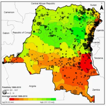
Many actors were only active in limited parts of the country. As we argue below, weather conditions play an important role in determining the intensity of the con‡ict in di¤erent regions. Figure5 displays the …ghting intensity and average climate conditions for di¤erent ethnic homelands in the DRC. The data used for generating this …gure is discussed in detail below.
3.2 Data
We build a panel dataset at the …ghting group - year level, covering the period 1998-2010 that includes both the o¢ cial years of the Second Congo War (until 2003) and its turbulent aftermath. To construct our main variables we draw on a variety of dataset.
Fighting e¤orts: We measure …ghting e¤orts at the group-year level using data from the Armed Con‡ict Location and Events Dataset (ACLED, 2012), a well established data source in the literature.14 This dataset contains 4765 geolocalised violent events taking place in the DRC between 64 …ghting groups over the 1998-2010 period. For each violent event, information is provided on the exact location, the date and the identities of the …ghting groups involved in the event. To construct our main variable of…ghting e¤ ort we take the sum over all …ghting events against other armed groups in which a given …ghting group is involved during a year. Our results are robust to restricting our attention to di¤erent types of events (e.g. only to battles) or to a variant of the variable focusing on the number of fatalities occurring in events involving a given armed group in a given year (e.g. drop all events with a below-median number of fatalities).
Alliances and enmities: Unique to the ACLED data is also the information on the compo-sition of each opposing side involved in a given event. Consider the following three examples: On the 18th of May 1999 a battle took place between "RCD: Rally for Congolese Democracy (Goma)" and "Military Forces of Rwanda", on one side, and the "Military Forces of Democratic Republic of Congo" on the other side. On the 13th of January 2000 there was a battle between "Lendu Ethnic Militia" and "Military Forces of Democratic Republic of Congo", on the one side, and "Hema Ethnic Militia" and "RCD: Rally for Congolese Democracy", on the other side. On the 3rd of February 2000, the "MLC: Congolese Liberation Movement" together with "Military Forces of Uganda" confronted the allied forces of the "Military Forces of Democratic Republic of Congo" and "Interahamwe Hutu Ethnic Militia".
While the ACLED data has been widely used in recent years to measure geo-referenced …ghting e¤orts, the dyadic information it contains about which groups …ght together or against each other in given events has received limited attention so far. To the best of our knowledge, our study is the …rst that exploits this information to construct a network of alliances and enmities. Using ACLED to construct the network of alliance and enmity links has the major advantage of covering smaller groups and militias that most qualitative case studies of the Second Congo War miss. However, ACLED cannot recover links between groups that may take place without them physically meeting in the battle…eld. Some such alliances may actually be very important, especially since some of the foreign actors only become involved sporadically in battle…elds. In order not to miss such links, we supplement the ACLED data with the alliance relationships listed in the Yearbook of the Stockholm International Peace Research Institute (SIPRI) (Seybolt, 2000).
In a nutshell, the two main variables of this dataset provide us with direct measures of our main theoretical variables, namely xt; the vector of equilibrium …ghting e¤orts in yeart, and A+[A
the adjacency matrices of alliances and enmities observed on the battle…eld. We measure xit;the
…ghting e¤ort of a group i in year t; as the total number of ACLED violent events the group participates to. From the matrix of alliances and enmities we are also able to retrieve to additional variables, "d-(#Enemies)", which corresponds to the numbers of enmity links, as well as "d+ (#Allies)", which captures the number of alliance links.
Other variables:
The following variables are used to generate the set of standard control variables and of Instru-mental variables (IVs). Below we shall describe in detail the exact speci…cation of controls and IVs.
- Government Organization: This variable takes a value of 1 for …ghting groups that are o¢ cial government organizations of one of the countries involved, and 0 otherwise. In particular, are coded as one the Military Forces of Burundi, Chad, Namibia, Rwanda, South Africa, Sudan, Uganda, Zambia and Zimbabwe.
- Foreign: This dummy variable takes a value of 1 for all foreign actors, and a value of 0 of all domestic …ghting groups that originate from the DRC.
- Fighting E¤ ort Outside the DRC: For all groups we also compute the total number of …ghting events in which they are involved outside the DRC. This proxies for the global scope of operation of a group.
3.3 Network of Fighting Groups in DRC
In this section, we discuss how we construct the network of alliances and enmities among the belligerent groups. We code two groups i; j; as being allied (i.e. a+ij =a+ji = 1) if they have been …ghting as brothers in arms in at least one event over the whole sample period, and, in addition, they have never fought on opposing sides in any event. Similarly, we code two groups as being enemy (i.e. aij =aji = 1) if they have fought on at least two occasions on opposing sides during the sample period, and have never been allied in any event.15 We code all other dyads as neutral (i.e. a+ij =aij = 0). This neutral coding includes dyads whose groups have fought at some point on the same side and at some other point on opposing sides.
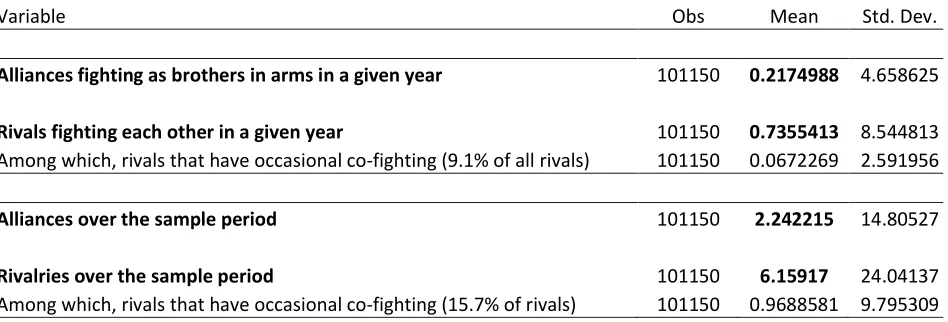
The links corresponding to these coding rules are described in Table 7. The upper part of the table reports statistics on an annual basis. In any given year roughly 1% of dyadic observations are reported as …ghting on the same or on opposite sides. This small proportion re‡ects the fact that big battles are relatively rare and that most groups are not necessarily involved in …ghting in every single year of the sample, though it is also possible that some events pass unrecorded. There are about 3.5 more enmities than alliances, re‡ecting the overall highly con‡icted situation in the DRC during the war period. In a limited number of cases (less than a tenth of the observations) we see inconsistencies: groups that have fought on at least two occasions on opposing sides have also fought, in at least one occasion, as brothers in arms against a common enemy in a given year. As discussed above, we code such instances as neutral.16 The lower part of the table reports statistics over the entire sample (1998-2010). This is the information we use to construct the network. Over the whole period, about 8% of dyads are coded as either allied or enemies, enmities are about 3 times more frequent than alliances, and about 15% of enmities have some occasional co-…ghting over the sample period. We view as reassuring the fact that the number of inconsistencies (i.e., the occasional …ghting as brother in arms of enemy groups) does not rise sharply when we consider the whole sample period is reassuring. For this reason, we focus on a time-invariant network.17
Assuming a time-invariant nature is by necessity subject to some caveats. However we some clear advantages to our procedure: First, a time-varying network would raise rampant concerns of reversed causation, due to past …ghting e¤orts a¤ecting future link formation. Second, using an "automatic" coding rule reduces the risk of perception bias in manual coding of links by the researcher. The exhaustive data from ACLED makes sure that even links between small players are recorded, which would surely be missed when using exclusively manual coding of links based on background readings. Third, our coding rule is conservative: It is likely that we code as neutral some dyads that are in fact allies or enemies but did not have the opportunity to participate into a common …ghting event (e.g. due to spatial distance). This issue is partly alleviated by adding the alliance links described by the specialists of SIPRI (Seybolt, 2000), but it is likely that many links remain missing. Such missing links create measurement errors that lead to attenuation bias in the estimates of the …ghting externalities (Chandrasekhar and Lewis, 2011). In our empirical analysis the 2SLS speci…cation alleviates this issue (thus, we expect the 2SLS coe¢ cients to larger than their OLS counterpart).
We document that our results are robust to other coding rules of alliances&enmities. First, our results go through if the coding thresholds are changed, e.g. when rivals with occasional
1 5
Given that in our setting by de…nition all groups are competing for larger shares of the pie, we require at least two instances of …ghting against each other to code two groups as rivals. Our results are robust to also coding as
rivals group that …ght on only one occasion against each other.
1 6As discussed below, our results are robust to alternative coding rules. 1 7
Variable Obs Mean Std. Dev.
Alliances fighting as brothers in arms in a given year 101150 0.2174988 4.658625
Rivals fighting each other in a given year 101150 0.7355413 8.544813
Among which, rivals that have occasional co-fighting (9.1% of all rivals) 101150 0.0672269 2.591956
Alliances over the sample period 101150 2.242215 14.80527
Rivalries over the sample period 101150 6.15917 24.04137
Among which, rivals that have occasional co-fighting (15.7% of rivals) 101150 0.9688581 9.795309
Figure 7: Descriptive Statistics of the Network Links
co-…ghting are coded as non-neutral (e.g. as enemy), or when groups are required to have had at least a n number of positive or negative interactions for being coded as having a positive or negative link. Second our results are robust to using of alternative data sources. In particular, in a robustness check we supplement our information with that provided in the "Non-State Actor Data" of Cunningham, Gleditsch and Salehyan (2013).
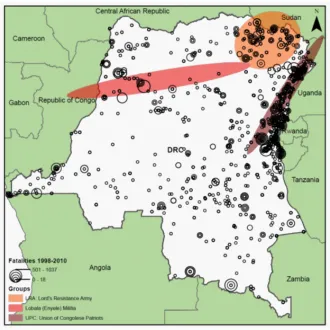
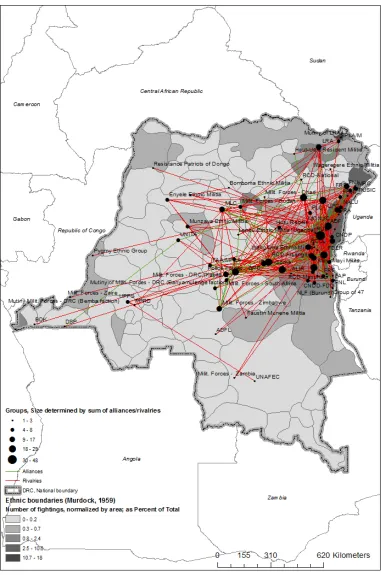
The summary statistics of the network is displayed in Table 8. We also display the network graphically with the aid of maps of the DRC: Figure 9 covers the whole of DRC, while Figure 10 focuses on the particularly on Eastern Congo and the disputed Kivu region. In the maps, the points indicate the centers of action of the various groups and the green and red lines show, respectively, alliance and enemy links. The polygons capture the homelands of di¤erent ethnic groups and the polygons painted in darker red identify areas characterized by higher …ghting intensity.
3.4 Structural Estimation and Exclusion Restriction
In this Section, we present the econometric model. We consider a con‡ict with a given network that repeats itself over several years. We abstract from reputation and repeated game e¤ects, and assume that each period is a one-shot game. Although the network is stable, there is variation in the outcome, driven by di¤erent realization of group-speci…c shocks. The inclusion of shocks has the dual purpose of matching more credibly real data, and of providing econometric identi…cation. More precisely, we elaborate on the model of section 2.5 where OP,'it;is impacted by group-speci…c shocks,'~it (equation (15)) that are now assumed to capture observable and unobservable (for the econometrician) heterogeneity. More formally, we let '~it =z0it +ei+ it, wherezit is a vector of
observable shifters with coe¢ cients andei is a time-invariant group-speci…c unobservable shifter and itis a iid, zero-mean unobservable shifter. Weather shocks are examples of observable shifters
zit that will be key in our instrumental variable strategy; leadership or the moral of troops are
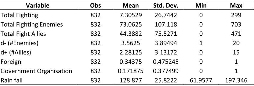
Variable Obs Mean Std. Dev. Min Max
Total Fighting 832 7.30529 26.7442 0 299
Total Fighting Enemies 832 73.0625 107.118 0 703
Total Fight Allies 832 44.3882 75.5271 0 471
d- (#Enemies) 832 3.5625 3.89494 1 20
d+ (#Allies) 832 2.28125 3.13172 0 15
Foreign 832 0.34375 0.475245 0 1
Government Organisation 832 0.171875 0.377499 0 1
Rain fall 832 128.877 25.8222 61.9577 197.346
Figure 8: Summary statistics
Equation (15) yields, then, the following expression for the OP of group iin yeart:
'it=xit+ 2 4
n X
j=1 a+ijxjt
n X
j=1 aijxjt
3
5+z0it +ei+ it: (21)
The equilibrium characterization of the equilibrium follows the discussion in Section 2.5). Recall, in particular that the share of the prize appropriated by each group is independent of'~it:In particular,
n X
i=1 'it=
2
41 Pn 1
i=1 1+ d+1
i di
3
5 V; (22)
which is identical to Equation (6) in the model without heterogeneity. Hence, the total economy-wide OP is fully characterized by the time-invariant network structure, ( ; ; di ; d+i ), being inde-pendent of the realizations of individual shocks (zit; ei; it). This result simpli…es substantially the
estimation procedure because it implies that there is no macro-feedback of unobserved heterogeneity on the equilibrium individual e¤orts.
Combining individual best-response (17), de…nition (21), and the equilibrium aggregate condi-tion (22) we obtain the equilibrium e¤ort for each agenti
xit= n X
j=1
a+ijxjt+ n X
j=1
aijxjt z0it +ui it: (23) where the time-invariant term of unobserved individual heterogeneity is de…ned as
ui ei+ (G) (1 (G)) i(G) V (24)
1. Correlated E¤ ects – in the structural equation (23) the term of time-invariant unobserved heterogeneity ui correlates potentially with neighbor …ghting e¤orts xjt through the deep
parameter (G) (an issue called "correlated e¤ects" in the literature). Contrary to most existing papers, the panel structure of our data makes possible the inclusion of group speci…c …xed e¤ects that absorbui.
2. Re‡ection Problem – The estimation of the …ghting externalities ; requires exogenous
sources of variations in allies/enemies …ghting e¤orts distinct from shifters of own …ghting e¤ort. The structural equation (23) makes clear that the neighbors’observable shifterszjtare
excluded fromxit: They do not a¤ect directly the …ghting e¤ortxitbut only indirectly through the observable …ghting e¤ort of the allies/enemies xjt:Hence, our identi…cation strategy can exploit exogenous shifters ofzjt as instruments of neighbor outcomesPnj=1a+ij xj, controlling for the shifters ofzit (in order to …lter out spatial correlation between shifters). The existing
literature (e.g. Bramoullé et al., 2009) usually exploits covariates of neighbors of neighbors because the neighbors covariates cannot be excluded from the structural equation; an issue we do not face here. However in robustness checks we also use observable shifters of neighbors of neighbors …ghting e¤orts as additional instruments.18
3. Instrumental Variables–Finding strong enough instruments that do not violate the exclusion restriction is not easy: While time-invariant potential candidate IVs would be multicollinear to the group …xed e¤ects, time-varying shocks occurring at the country level would violate the exclusion restriction. We consequently use time-varying climatic shocks (rainfall) impacting …ghting groups "homelands". As shown below, rainfall correlates indeed strongly with the allies’and enemies’…ghting e¤orts, and the F-statistic of the …rst stage of the 2SLS regression is above the conventional thresholds. In line with the empirical literature and historical case studies, we expect groups a¤ected by large positive rainfall shocks to …ght less, for two reasons. First, local rainfalls are associated with larger agricultural surplus that increases the reservation wages of productive labor and hence leads to a greater opportunity cost of …ghting. This channel linking rainfall to con‡ict has been documented by Miguel et al. (2004) and Vanden Eynde (2011), among others. Second, heavy rain imposes technical constraints on …ghting, e.g. by making troop transportation more di¢ cult (cf. for example, Rogall, 2013).
The exclusion restriction requires that rainfall taking place in the allies’and enemies’home-lands does not have a direct impact on …ghting e¤orts of a given groupiother than through the …ghting e¤orts’spillovers once we control for i’s own rainfall. Potential violation of the exclusion restriction could arise if there were intense within-country trade. For instance, a negative shock hitting crops in Western Congo could translate into strong price increases of agricultural products throughout the entire DRC, thereby a¤ecting …ghting in the Eastern part of the country. Such a channel may be somewhat plausible in a highly integrated country with large domestic trade. In a very poor country like the DRC a disintegrating government, very lacunary transport infrastructure and the disastrous security situation leads to very large transport costs reducing inter-regional trade for most goods, and leading to a very localized economy dominated by subsistence farming. Hence, in this context large-scale inter-regional economic spillovers are less plausible.
3.5 Estimates of the Fighting Externalities
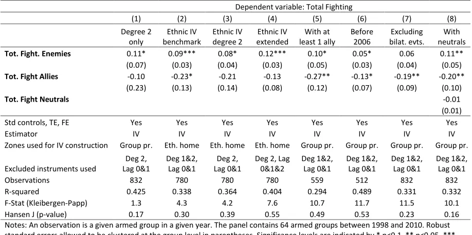
We now present the estimates of the structural equation (23) based on a panel dataset containing 64 armed groups between 1998 and 2010. The observational unit is a given armed group in a given year; in all speci…cations, the standard errors are clustered at the group level.
Table 1 reports the results from the baseline speci…cations. In Column (1) we start with an OLS speci…cation including group …xed e¤ects and year dummies. The total …ghting of enemies increase a group’s …ghting e¤ort, whereas the total …ghting of allies decreases its …ghting e¤ort. These results conform with the prediction of the theory, although the coe¢ cient of total …ghting of allies is not statistically signi…cant. In column (2) we control for the current and lagged rainfall in the center of a given group’s zone of activity, allowing for both linear and quadratic e¤ects. The results are unchanged.
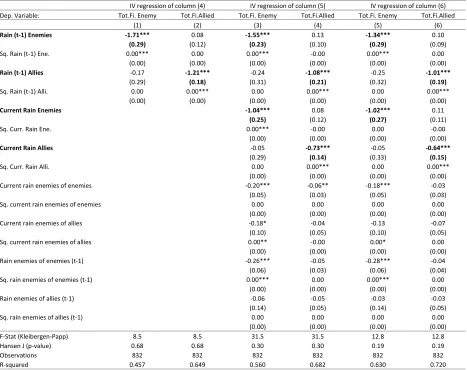
Column (3) aims at controlling other time-varying shocks a¤ecting …ghting at the group-level. Unfortunately, there are no data on such shocks (other than on weather conditions). Therefore, we postulate that common shocks unobserved to the econometrician have heterogenous e¤ects across groups that di¤er by some observable characteristics. More speci…cally, we build four broad time-invarying group characteristics and interact each them with year dummies. For instance, the intensity of international interventions to limit the in‡uence of foreign armies may have an especially noticeable e¤ect on foreign actors. Thus, construct a binary variables coding for foreign groups operating in DRC, and interact it with a time dummies. Another binary variables (also interacted with time dummies) captures groups a¢ liated to the DRC government - the activity of these groups may be a¤ected by …nancial aid or external political pressure exercised on Kinshasa government. The other two variables proxy for group size Note that we have no data on troop size.19 Therefore, we resort to two binary variables coding, respectively, large groups with at least 10 enemies (roughly the top decile of the sample), and groups …ghting at least 20 violent events per yearoutside the DRC (again, this corresponds to the top decile of the sample). In column (3) we include this battery of time-varying controls. The estimated coe¢ cients are stable, and more precisely estimated. The coe¢ cient oftotal …ghting of allieshas now a p-value just above 5 percent. In column (4) we report the result from the second stage of a 2SLS speci…cation including (lagged) weather shocks but no other time-varying control variables. In this speci…cation, total …ghting of enemies and total …ghting of allies are instrumented, respectively, by the one-year lag of average rainfall in enemies and allies homelands (where both a linear and square terms are included in the regression). The coe¢ cients of the variables of interest have the expected sign and are signi…cant. The coe¢ cients are larger than in the OLS regressions, suggesting that the non-instrumented speci…cation su¤ers from a severe estimation bias due to network externalities. Note that the direction of the bias is unclear because the two …ghting externalities have opposite signs, and the network externalities compound them in a complicated way. Columns (1) and (2) in Table 2 display the …rst stage regressions for thetotal …ghting of enemiesandtotal …ghting of allies. We see that the instruments have statistically signi…cant coe¢ cients, with the expected sign, but the overall statistical power is slightly too weak (Kleibergen-Paap F-stat equal to 8.5). The null hypothesis of the Hansen J test is not rejected indicating that the overidenti…cation restrictions are valid. In column (5) of Table 1, we include a larger set of instruments comprising current-year rainfall (linear and quadratic terms) as well as current and lagged rainfalls of degree 2 neighbors (i.e. enemies of enemies and of enemies of allies).20 The second-stage coe¢ cients are stable and
1 9
Such data only exist for a small subset of the 64 groups operating in DRC over the 1998-2010 period, see the International Institute of Strategic Studies (IISS) or the Small Arms Survey (SAS).
2 0