Online Appendix for
The Geography of Inter-State Resource Wars
Francesco Caselli, Massimo Morelli, and Dominic Rohner
July 24, 2014
1
Endogenous Armament
The model is identical to the model in the paper, except that we introduce a new stage
at the very beginning. In this new …rst stage, each country decides how much to invest in
armaments. Armament spending by country i is denoted by Wi. It carries a cost (Wi).
The two countries’spending in armaments a¤ect the distribution ofZ.
Assumption 1.1 Z is a continuous random variable with domainR, densityf(Z;WA; WB), and cumulative distribution function F(Z;WA; WB).
Following the choices of WA and WB, the game proceeds exactly as in the baseline
model. Hence, if the outcome is peace, the payo¤s are RA (WA) for country A, and
RB (WB) for countryB. If there has been a war, the payo¤s are:
UAC = RAI(Z > GA) +RBI(Z > GB) +cA (WA);
UBC = RAI(Z < GA) +RBI(Z < GB) +cB (WB):
whereI is an indicator function.
In the second stage of the game the players takeWAandWB as given. Hence, following
the identical logic of the Proposition in the main text, we see that the probability of peace
is
P(GA; GB; RA; RB;WA; WB) = H( x)H(x)
and it is decreasing in the absolute value ofx.
In the …rst stage, each country i choosesWi. Country B’s problem is
max
WB
8 < :
[1 P(GA; GB; RA; RB;WA; WB)] [RAF(GA;WA; WB) +RBF(GB;WA; WB)]
+P(GA; GB; RA; RB;WA; WB)RB (WB)
9 = ;;
which can be rewritten as
max
WB f
[1 H( x)H(x)]x+RB (WB)g:
From this, we see that even in the two-stage game with endogenous arming e¤ort our
Remark 2 in the baseline model still holds: the case RA = 0 is isomorphic to the case
GA ! 1, and the case RB = 0 is isomorphic to GB ! 1. In other words, we can just
write WA as a function of GA and GB, and WB as a function of GA and GB. Then we
can de…ne a function (Z;GA; GB) F(Z;WA(GA; GB); WB(GA; GB)). Accordingly, the
probability of peace is
P(GA; GB) = H( x)H(x)
x = RB RB (GB;GA; GB) RA (GA;GA; GB):
As in the baseline model, we set RA; RB 2 f0;1g. We then obtain the following
predictions:
Proposition 1.1
(i) P(GA;1) P( 1;1);
(ii) @P(GA;1)=@GA 0if 1(GA;GA;1)> 2(GA;GA;1); (iii) P(GA; GB) P( 1;1);
(iv) P(GA;1) P(GA; GB) if and only if (GA;GA;1) 1 (GB;GA; GB)
(GA;GA; GB) (GA;GA;1);
(v) @P(GA; GB)=@GA 0 if and only if either 1 (GA;GA; GB) (GB;GA; GB)
0 and 1(GA;GA; GB) [ 2(GA;GA; GB) + 2(GB;GA; GB)] or 1 (GA;GA; GB)
(GB;GA; GB)>0and 1(GA;GA; GB)< [ 2(GA;GA; GB) + 2(GB;GA; GB)] ;
where 1(x;y; z)is the derivative of with respect tox, and 2(x;y; z)is the derivative
The proposition says that parts (i) and (iii) of the original proposition in the baseline
model are entirely robust to endogenous arming e¤ort (or any other endogenization of
the distribution of contest success). This is not surprising. Even if the two countries can
respond to oil discoveries by arming there is still a country who (weakly) expects to “do
better” from war, and con‡ict unambiguously goes up relative to the case where neither
country had oil.
Part (ii) is robust as long as 1(GA;GA;1)> 2(GA;GA;1). Clearly 1(GA;GA;1)>
0 so our original prediction fails only if 2(GA;GA;1) is negative and large in absolute
value. We can think of 1as the “direct”e¤ect of movingA’s oil towards the border, which
is to make A’s oil within easier reach for country B. On the other hand, 2(GA;GA;1)
is the “indirect” e¤ect that occurs as the two countries endogenously change their
arma-ments. For 2 to be negative it must be the case that the relative military strength of
country A increases as country A’s oil moves towards the border. This may be the case,
for example, if country A responded to the movement of the oil towards the border by
ramping up military spending much more than country B. Clearly both countries may
have an incentive to increase military spending as countryA’s oil moves towards the
bor-der, but there is no particular reason to presume that country A will do more - at any
rate not so much more that 2 becomes su¢ ciently negative for the indirect e¤ect from
endogenous arming to overcome the direct geographic e¤ect. In the special case where the
two countries have the same marginal cost from arming we expect 2 = 0, and our original
proposition goes through unchanged.
The notion of “direct” and “indirect” e¤ects helps interpreting the new parts (iv)
and (v) as well. To interpret part (iv) note that we can think of the quantity 1
(GB;GA; GB) (GA;GA; GB) as country A’s (expected) net territorial gain from
con-‡ict after the discovery of oil in country B, and of (GA;GA;1) as country A’s
(ex-pected) loss (equal to B’s expected gain) before B’s oil discovery. Then the
proposi-tion says that: (i) if country A continues to be the net territorial loser after the
discov-ery of oil in country B [1 (GB;GA; GB) (GA;GA; GB) 0], then the new
discov-ery has reduced con‡ict unless B’s discovery of oil on its own soil has increased B’s
bene…ts from con‡ict compared to when only A had oil. Clearly the direct e¤ect of
(GA;GA; GB) = (GA;GA;1)]. What is required is that B increases its military
spend-ing relative toA so much as to overturn the direct e¤ect. Once again, it is not clear why
this should be the case. (ii) If instead country A becomes the net territorial winner
af-ter the new discovery[1 (GB;GA; GB) (GA;GA; GB)>0], then the discovery in the
second country has reduced con‡ict if B’s net bene…t from con‡ict before the discovery
exceeds A’s bene…ts after. As in the baseline model, we would expect this to be the case
in most scenarios, since in the two-oil scenario both countries have something to lose from
con‡ict, while in the one-oil scenario the net territorial winner has no territorial losses to
fear.
This reasoning also allows us to easily interpret part (v). If 1 (GA;GA; GB)
(GB;GA; GB) 0then A is the territorial loser, and the relevant condition for increased
con‡ict from an increase inGA, 1(GA;GA; GB) [ 2(GA;GA; GB) + 2(GB;GA; GB)],
says that the direct e¤ect 1 >0must exceed any indirect e¤ect from endogenous arming.
In particular, to reverse the predictions of the baseline model the territorial loser must
respond to a movement of its oil towards the border by a disproportionate increase in
armaments (so that 2 is not only negative but also large in absolute number). Again, it
is hard to see why this should generally be the case. (The case were B is the territorial
loser is entirely symmetric, of course).
2
A Dynamic Model
In this section we show that the sharp predictions of our model summarized in Proposition
1 extend to a dynamic setting in which a war can be followed by other wars. Given that
in the model in the main text a war has a stochastic outcome, the dynamic model will
continue to have that feature, but we need to "discretize" the model in order to avoid
having to handle a continuum of realizations of the state variable, namely the border.
In particular, we now switch to a “…nite”geography which identi…es the world with the
segment [ Z; Z], Z > 0; and assume that the border can take only 5 values (locations),
namely Z, Z ; Z0; Z , and Z, with Z0 = 0, Z >0.1 Given any distribution of oil on
the space, we need to study the equilibrium strategies at the initial state of the world,
Z0 (the middle), fully anticipating the continuation war-or-peace behavior that would be
taken at all other nodes Zt = Z orZt = Z if reached as a consequence of a war. The
game has an in…nite number of periods.
In case of war let pZ denote the probability of a change of the state "one step to the
right" andqZ the probability of a shift "one step to the left", with 1 pZ qZ being the
probability of remaining at borderZ. We make the following two assumptions:
Assumption 2.1 (Equal strength) pZ =qZ =p 8z = Z ; Z0; Z ;p Z =q Z =pZ =
qZ = 0.
The expression p Z = q Z = pZ = qZ = 0 means that once a country is fully
conquered it ceases to exist, implying that the border will never change anymore. The
present discounted value of being conquered (and ceasing to exist) is normalized to zero,
i.e. VA(Z = Z) = VB(Z =Z) = 0.
Assumption 2.2 (Equal cost of war) At time 0 there is a realization of the net bene…t parameter c, from a distribution H on the real line. This parameter remains constant for
the subsequent periods and it is the same for both countries.
Both the equal strength assumption and the equal cassumption can be removed, only
at the cost of more complex algebra. With these two assumptions we can focus exclusively
on the role of the geographic asymmetries.
Consistent with the basic model, assume that the instantaneous utility of a country
depends only on oil rents: uA(Zt) =RAI(Zt> GA) +RBI(Zt > GB), where Gi, i =A; B
denotes the location of an oil well on the line, andI is an indicator function. It is symmetric
forB.
The game starts at time 0 at Z0 and then the two players are free to decide in every
subsequent period whether to accept the current state of the world (border) or try to change
it with a war. We shall assume that in every period one of the two players is randomly
selected with equal probability to move …rst. This assumption serves the purpose of ruling
out all weakly dominated equilibria.2
The timing under war is such that at the beginning of the war period the net bene…t
of warc(negative on average under most realistic assumptions on the distribution ofc) is
received, and in the same period the border shifts or stays. The instantaneous utility of
the period is the one corresponding to the new border.
In terms of oil endowments, in order to mimic the situations discussed in the main text,
we consider the following possibilities:
–Case No-No: RA =RB = 0 (no oil);
–Case Far-No: Ri = 1, R i = 0, jGij > Z (oil only in one country, far from the border);
–Case Close-No: Ri = 1,R i = 0,jGij< Z (oil only in one country, near the border);
–Case Far-Far: RA =RB = 1, jGAj> Z , jGBj> Z (oil in both countries, far from the border);
–Case Close-Close: RA =RB = 1, jGAj < Z , jGBj< Z (oil in both countries, near the border);
–Case Far-Close: RA =RB = 1, jGij > Z , jG ij < Z (oil in both countries, one far and one near the border);
where istands for B (A) when i stands forA (B).
Given the equal strength assumption and the equal cost of war assumption, the three
asymmetric cases can be described just in terms of endowment and distance: both case
Far-No and case Close-No are asymmetric in terms of endowment, but the latter case has
closer oil to the initial border; case Far-Close does not have endowment asymmetry but
only distance asymmetry.
Let us consider the Markov Perfect Equilibrium of this game, which allows players to
consider only payo¤ relevant information from the history of play.This standard selection
gives prominence to the state variable "border" alone.
Proposition 2.1 There exists a unique Markov Perfect Equilibrium (MPE). In the MPE, the probability of war in period 0 is:
1. Highest in case Close-No;
2. Lowest in cases No-No, Far-Far, and Close-Close;
Proof.
At the two absorbing one-country states the value for the unique surviving state is
VB( Z) = VA(Z) = kR=(1 ), where k denotes the number of oil wells in the whole
region, which can take values 0,1,2.3
Let us now describe the values at the other states. For peace in every period,
Vi(Z) = u
i(Z)
1 ; i=A; B; Z = Z ; Z0; Z :
Besides these "value of peace" simple expressions, denote by Wi(Z) the continuation
expected value of a war starting from a borderZ.
Assume …rst that in states Z0 and Z there will always be peace, and let us derive the
indi¤erence condition in state Z between war and peace. We know that VA( Z ) =
(uA( Z ))=(1 ), and will set VA( Z ) = WA( Z ) to …nd the threshold. Given that
WA( Z ) =c+p u
A(Z
0)
1 + (1 2p) u
A( Z ) + VA( Z ) ;
the threshold for indi¤erence is
cA = p
1 [2u
A( Z ) uA(Z
0)]:
Assume now that at states Z and Z there will always be peace. Solving for the
indi¤erence threshold at stateZ0 yields:
cA0 = p 1 (2u
A(Z
0) uA( Z ) uA(Z )):
Assuming that at states Z and Z0 there will always be peace, solving for the
indif-ference threshold at stateZ yields:
cA+ = p
1 (2u
A(Z ) uA(Z
0) kR):
The thresholds for countryB are analogous.
Considercase No-No: In the absence of oil, the thresholds de…ned above are
cA =cA0 =cA+ =cB =cB0 =cB+ = 0:
For any c < 0, i.e., whenever the net bene…ts of war are negative, peace is the unique
Markov Perfect Equilibrium. In fact, with c < 0, not only it is an equilibrium to stay
peaceful given the (consistent) assumptions at the adjacent nodes, but it remains a best
response in case 0 even when at an adjacent node there is war.
On the other hand, wheneverc >0, given that the expected value of eternal peace is 0,
while with positivecthe expected value of seeking war is strictly positive for both players,
the unique MPE involves war at every node.
Consider now case Far-No. The thresholds become:
cA = p
1 R;
cA0 =cA+ =cB0 =cB+ = 0;
cB = p
1 R:
Clearly A would always have (weakly) lower incentives to start war than B. Hence, we
can focus onB’s incentives, which are the binding constraint for the existence of a Markov
Perfect Equilibrium with peace. Clearly, when c < 1p R, there will always exist a MPE
with peace (note that this is a higher cost of war with respect to the one needed in case
0), and no other MPE can exist.
Now consider c > 1p R. Assuming war in node Z and peace in node Z , we can
deriveB’s indi¤erence condition in nodeZ0. The value of a war in state Z0 is
WB(Z0) =c+p(uB( Z ) + WB( Z )) +p
uB(Z )
1 + (1 2p)
uB(Z
0)
where
WB( Z ) =c+p R
1 +p
uB(Z0)
1 + (1 2p)(u
B( Z ) + WB( Z ));
WB( Z ) = c+p
R
1 +p
uB(Z
0)
1 + (1 2p)u
B( Z )
1 (1 2p) :
Imposing the indi¤erence conditionWB(Z0) = VB(Z0) = (uB(Z0))=(1 ), we obtain
c= p
1 (1 3p)
p
1 R
Note that 1 (1 3p p) <1 always holds. Hence, for 1p R < c < 1 (1 3p p)1p R, there will
be war at state Z , but not at states Z0 and Z . For c slightly above 1 (1 3p p)1p R
there will be a zone where there is war in states Z and Z0, but peace at state Z .
What matters are the war incentives at state Z0, and hence we can conclude that in
case a war will occur i¤c > 1 (1 3p p)1p R.
Let us now analyzecase Close-No, for which the peace in all periods thresholds derived
above become
cA = p
1 R; c
A
0 =
p
1 R; c
A
+ = 0;
cB = p
1 R; c
B
0 =
p
1 R; c
B
+ = 0:
When c < 1p R, there will always be peace. Now suppose that c is a bit larger.
Assume that at Z there will be war; at Z instead peace. Let us compute the condition
under which B is indi¤erent between peace and war atZ0.
Knowing the values at the boundaries, we also know thatVB(Z
0) = (uB(Z0))=(1 )
and VB(Z ) = (uB(Z ))=(1 ). The value of war atZ
0 is
WB(Z0) = c+p[uB( Z ) + WB( Z )] +p
uB(Z )
1 + (1 2p)
uB(Z
0)
1 ;
where
WB( Z ) =c+p R
1 +p
uB(Z0)
1 + (1 2p)[u
B( Z ) + WB( Z )]:
From the conditionWB(Z
0) = VB(Z0) = (uB(Z0))=(1 ) it follows that
c= 1 (1 p)
1 (1 3p)
p
1 R:
Note that 11 (1 3(1 pp))1p R < 1 (1 3p p)1p R, which implies that the ex ante probability
For consistency with the assumption of war at Z , we need to also derive the
indif-ference threshold forA at Z when there is war at nodeZ0, and peace at Z . The value
of war at Z is
WA( Z ) =c+p[uA(Z0) + WA(Z0)] + (1 2p)
uA( Z )
1 ;
where
WA(Z0) =c+p
uA( Z )
1 +p
uA(Z )
1 + (1 2p)[u
A(Z
0) + WA(Z0)]:
FromWA( Z ) = VA( Z ) = (uA( Z ))=(1 ), we obtain
c= 1 (1 p)
1 (1 3p)
p
1 R:
This means that for c > 11 (1 3(1 pp))1p R at Z there is war, as assumed for computing
B’s threshold at node Z0.
In summary, incase Close-No war will occur atZ0 i¤c > 11 (1 3(1 pp))1p R.
Following similar steps, it is possible to show that case Far-Far and case Close-Close
are equivalent to case No-No.
Finally, consider case Far-Close, with B having oil close to the border. The peace in
all periods thresholds become
cA = p
1 R; c
A
0 =
p
1 R; c
A
+ =
p
1 R;
cB = p
1 R; c
B
0 =
p
1 R; c
B
+ =
p
1 R:
Clearly, B has always lower incentives to attack at Z0 than A given the assumptions
at the adjacent nodes. So we need to check the incentives of A to attack. Now compute
the indi¤erence threshold ofA at Z0, assuming war at both adjacent states. The value of
war at Z0 is
WA(Z0) =c+p(uA( Z ) + WA( Z )) +p(uA(Z ) + WA(Z )) + (1 2p)(
uA(Z
0)
1 );
where
WA( Z ) = c+pu
A(Z
0)
1 + (1 2p)(u
A( Z ) + WA( Z ));
WA(Z ) =c+p 2R
1 +p
uA(Z0)
1 + (1 2p)(u
FromWA(Z0) = VA(Z0)) = (uA(Z0))=(1 ), we obtain
c= pR
1 (1 4p):
Again, we need to check for consistency that at Z and Z B will indeed stage war,
given war at Z0. Analogous computations yield that indeed B is indi¤erent between war
and peace at Z and Z in the presence of war at Z0 when
c= 1 (1 p)
(1 (1 3p))(1 )pR:
Given that unambiguously
1 (1 p)
(1 (1 3p))(1 )pR <
pR
1 (1 4p);
we con…rm that indeedB stages war at Z and Z , as assumed, when c > 1 pR(1 4p).
In sum, incase Far-Close war occurs at Z0 i¤c > 1 pR(1 4p).
Now compare the case Far-Close threshold c= 1 pR(1 4p) for war atZ0 to the
thresh-olds we found before: 1 (1 4pR p) > 11 (1 3(1 pp))1p R, which implies that war is more likely
incase Close-No than in case Far-Close.
In contrast, whether war is more likely incase Far-Close orcase Far-No is ambiguous,
as one cannot sign 1 (1(1 4)p) 7 1 (1 3p p).
End of Proof of Proposition 2.1
Note that the probability of war at time 0 in case Far-No can be higher or lower than
that in case Far-Close, depending on parameter values. The ambiguity is due to the fact
thatcase Far-No is endowment asymmetric, whilecase Far-Close is endowment symmetric
but has the close oil e¤ect that is missing incase Far-No.
Beside proposition 2.1, which serves the purpose of a robustness check of the main
results of our static theoretical model, this dynamic extension allows to make some extra
predictions:
Corollary 2.1 Conditional on observing a war at time 0, the probability of another war next period is higher if the …rst period war is won by the attacker than when it is won by
Given that the attacker is (in this equal strength and equal cost-bene…t benchmark)
always the country that is either oil less or at least has no oil close to border, while the
target country has oil, then if the attacker wins the other country will have roughly the
same incentives to attack back, whereas if the defender wins, then the border shifts away
from the oil, reducing the incentives to attack by the initial attacker.
3
Clustering at the Country Level
In the main body of the paper the standard errors are clustered at the country-pair level,
which is standard practice in literatures focusing on dyadic relationships (e.g. the vast
literature on gravity models in international trade, as well as of course much of the empirical
literature on international con‡ict). One criticism of this approach (which applies to nearly
all contributions in those literatures as well) is that it treats two di¤erent dyads featuring
the same country as independent observations. This suggests that it could be preferable
to have some sort of country-level clustering.
In a gravity-trade setting, Cameron, Gelbach, and Miller (2011) propose to use their
multi-clustering approach, where the …rst country in each pair is assigned to one cluster
and the second country to a second cluster. Spolaore and Wacziarg (2009) do the same in
an application where the dyadic outcome is the di¤erence in development between the two
countries.
As can be seen in Table 1 below, our results are very robust to applying the Cameron
et al. multi-clustering approach, treating country A and country B as di¤erent clusters.
Nevertheless, this approach is actually quite problematic. Whenever one uses a dyadic
data set, there will always be some countries that necessarily have to appear as country A
in some observations, and as country B in others. Clustering at the “country A, country
B” level will therefore create (for many countries) two separate clusters, one when the
country appears as country A, and one when it appears as country B. For this reason,
the multi-clustering approach is really not suitable to dyadic settings when one wants to
cluster at the country level.
Fafchamps and Gubert (2007) propose an alternative in the context of individual-level
data in a village-network setting. Their proposal looks more promising but –even in the
method to estimate standard errors.4 Those authors who have used it, have tended to …nd massive losses of signi…cance using Fafchamps-Gubert clustering. Needless to say that the
technique is unheard of in the international context, even though it is potentially applicable
to the entirety of the enormous trade literature on gravity equations, where the problem of
each country appearing in multiple dyads also applies (as well as in the literature on war,
of course). We therefore feel that the Fafchamps-Gubert method has not been adequately
“road tested”by the literature for us to make the big leap of adopting it as our benchmark
method. But we report results using this method in Table 2 of this appendix. Consistent
with the sparse references to results using this method in the network literature, we also
…nd a massive increase in estimated standard errors. However, even with this method some
of our core results survive, or remain very close to the margin of signi…cance.
4
Results with Region x Year Fixed E¤ects
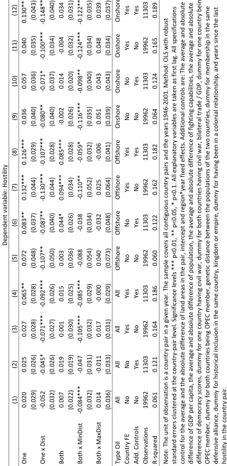
Results with …xed e¤ects for world regions interacted with the year …xed e¤ects are reported
in Table 3.
5
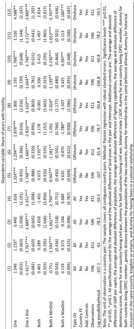
Results with Cross-Section of Country Pairs
Results obtained after collapsing the panel into a simple cross-section of country pairs,
where all variable values now correspond to the averages over the 1946-2001 period, are
reported in Tables 4 (OLS estimates) and 5 (Poisson regressions).
References
Cameron, Colin, Jonah Gelbach, and Douglas Miller, 2011, “Robust Inference with
Multi-way Clustering,”Journal of Business and Economic Statistics 29, 238-249.
Fafchamps, Marcel and Flore Gubert, 2007, “The Formation of Risk-Sharing
works,”Journal of Development Economics 83, 326-50.
Spolaore, Enrico and Romain Wacziarg, 2009, “The Di¤usion of Development,”
Dependent variabl e: Hostili ty (1) (2) (3) (4) (5) (6) (7) (8) (9) (10) (11) (12) One 0. 034 0. 029 0. 049 0. 077 ** 0.087* 0. 081 ** 0. 143 ** 0.124* ** 0. 048 0. 063 0. 058 0.132* ** (0.032) (0.029) (0.030) (0.033) (0.051) (0.041) (0.063) (0.047) (0.043) (0.040) (0.037) (0.050)
One x Dist
-0.050* -0. 044 -0.073* ** -0.086* ** -0.107* -0. 087 ** -0. 138 ** -0. 118 ** -0. 079 ** -0.072* -0.103* ** -0.137* ** (0.031) (0.028) (0.026) (0.032) (0.056) (0.043) (0.065) (0.046) (0.039) (0.040) (0.033) (0.048) Both 0. 022 0. 028 0. 034 0.045* 0. 023 0.048* 0.110* ** 0. 073 ** 0. 009 0. 024 0. 020 0. 047 (0.025) (0.023) (0.032) (0.026) (0.032) (0.028) (0.042) (0.032) (0.029) (0.024) (0.037) (0.031)
Both x Min
Dist -0. 077 ** -0. 044 -0.105* ** -0. 089 ** -0. 088 ** -0. 028 -0. 107 ** -0.066* -0.102* ** -0. 096 ** -0.122* ** -0.125* ** (0.036) (0.035) (0.036) (0.038) (0.043) (0.031) (0.052) (0.034) (0.036) (0.039) (0.034) (0.041)
Both x Ma
xDist 0. 026 -0. 014 0. 016 0. 004 0. 048 -0. 048 0. 012 -0. 010 0. 059 0. 042 0. 047 0. 043 (0.042) (0.039) (0.032) (0.036) (0.060) (0.046) (0.068) (0.046) (0.043) (0.045) (0.034) (0.042) Type Oil All All All All Offshore Offshore Offshore Offshore Onshore Onshore Onshore Onshore Country FE No No Yes Yes No No Yes Yes No No Yes Yes Add. Co ntrol s No Yes No Yes No Yes No Yes No Yes No Yes Observations 1996 2 1130 3 1996 2 1130 3 1996 2 1130 3 1996 2 1130 3 1996 2 1130 3 1996 2 1130 3 R-squared 0. 019 0. 090 0. 145 0. 158 0. 020 0. 091 0. 145 0. 156 0. 021 0. 092 0. 146 0. 160
Note: The unit of observation is
a country pair in a given year. The sample covers all co
ntiguous countr
y pairs and the years
1946
-2001.
Method: OLS with r
obust s
tandard
errors clustered at the leve
ls of "first
-country in the
dyad" and "second
-cou
ntry i
n t
he dyad". Significance levels *** p<0.01,
** p<0.05, * p<0.1. All explanatory variables
are taken a
s first lag
. All
specificati
ons contr
ol for th
e average and the absolut e di fference of land areas in th
e pair, int
ercept and annual time dummies. Additional
controls
are: The average and absolute difference of GDP per capita, the average and absolute difference o
f population, the average an
d absolu
te difference of fighting ca
pabilities,
the average an
d absolute d
ifference of dem
ocracy sc
ores, dumm
y for one cou
ntr
y having ci
vil war
, du
mmy for b
oth c ountries having civil war , bilatera l tra de / GDP,
dummy for one country being OPEC member, dummy for both countries being OPEC member, genetic distance between the populations
of the two c
ountries, dum
my for
membe
rshi
p in the same d
efensive allia
nce, dummy for historical inclusion in the same country, ki
ngd
om or em
pire, dummy for having bee
n in a colonial relationship, and
years since the last hostility in the c
Depen den t va riab le : H ostili ty (1) (2) (3) (4) (5) (6) (7) (8) (9) (10) (11) (12) One 0.0 34 0.0 29 0.0 49 0.077* 0.0 87 0.081* 0.143* * 0.124* * 0.0 48 0.0 63 0.0 58 0.132* * (0.033) (0.030) (0.034) (0.040) (0.055) (0.043) (0.068) (0.052) (0.046) (0.041) (0.042) (0.059)
One x Dist
-0.0 50 -0.0 44 -0.073* * -0.086* * -0.107* -0.087* -0.138* * -0.118* * -0.079* -0.072* -0.103* * -0.137* * (0.034) (0.028) (0.032) (0.038) (0.060) (0.045) (0.068) (0.050) (0.044) (0.040) (0.040) (0.057) Both 0.0 22 0.0 28 0.0 34 0.0 45 0.0 23 0.048* 0.110* * 0.073* * 0.0 09 0.0 24 0.0 20 0.0 47 (0.029) (0.024) (0.034) (0.032) (0.032) (0.027) (0.044) (0.034) (0.032) (0.026) (0.038) (0.034) Both x Min Dist -0.077* * -0.0 44 -0.105* ** -0.089* * -0.088* ** -0.0 28 -0.107* * -0.066* -0.102* ** -0.096* * -0.122* ** -0.125* ** (0.034) (0.037) (0.038) (0.041) (0.025) (0.034) (0.052) (0.034) (0.035) (0.043) (0.039) (0.047) Both x Ma xDis t 0.0 26 -0.0 14 0.0 16 0.0 04 0.0 48 -0.0 48 0.0 12 -0.0 10 0.0 59 0.0 42 0.0 47 0.0 43 (0.046) (0.042) (0.036) (0.042) (0.046) (0.045) (0.069) (0.047) (0.047) (0.050) (0.039) (0.052) Type Oil All All All All Offshore Offshore Offshore Offshore Onshore Onshore Onshore Onshore Country FE No No Yes Yes No No Yes Yes No No Yes Yes Add. Cont rols No Yes No Yes No Yes No Yes No Yes No Yes Observations 199 62 113 03 199 62 113 03 199 62 113 03 199 62 113 03 199 62 113 03 199 62 113 03 R-squared 0.0 76 0.1 31 0.1 95 0.1 96 0.0 77 0.1 32 0.1 95 0.1 93 0.0 78 0.1 33 0.1 96 0.1 98
Note: The unit of observation is a countr
y pair in a given year. The sample c
overs all contiguous countr
y pairs and the years
1946 -200 1. Me thod: OLS wi th r obust sta nda rd
errors clustered at
the country le
vel.
Significanc
e levels *** p<0.
01, ** p<0.05,
* p<0.1. All explanat
ory variables are
taken as firs
t lag. All sp
ecifications cont
rol for
th
e
average and the absolute d
ifference of land areas in the pair, intercept
and annual time dummies. Add
itional controls a
re: The averag e an d absolu te diff erenc e of GDP per
capita, the averag
e and abs
olute differenc
e of population, the
average and
absolute differ
ence of fighting c
apa
bilities, the
average and ab
solute difference of dem
ocracy scores , dum my f or on e cou ntry ha vin g c ivil w ar, du mmy for b oth cou ntri es ha vin
g civil w
ar, bi late ral tra de / G DP, du mmy for on e cou ntry bein g O PEC m ember , d ummy for
both countries being OPEC
member, genetic distance between the populations of the two countries, dummy for membership in the
same d efensi ve allia nc e, du mmy for
historical inclusion in the same country, kingd
om or empire, dum
my for having been in a colonial relationshi
p, and years sinc
e the last
hostility in the c
Dependen t vari abl e: Hostil ity (1) (2) (3) (4) (5) (6) (7) (8) (9) (10) (11) (12) One 0.020 0.025 0.027 0.065* * 0.072 0.083* * 0.132* ** 0.126* ** 0.036 0.057 0.040 0.130* ** (0.0 29) (0.0 26) (0.0 28) (0.0 28) (0.0 48) (0.0 37) (0.0 44) (0.0 29) (0.0 40) (0.0 36) (0.0 35) (0.0 43)
One x Dist
-0.052 -0.045* -0.071* ** -0.092* ** -0.107* * -0.087* * -0.130* ** -0.107* ** -0.080* * -0.071* -0.100* ** -0.148* ** (0.0 32) (0.0 26) (0.0 27) (0.0 26) (0.0 50) (0.0 40) (0.0 44) (0.0 28) (0.0 40) (0.0 37) (0.0 34) (0.0 40) Both 0.007 0.019 0.001 0.015 0.003 0.044* 0.094* ** 0.085* ** -0.002 0.014 -0.004 0.034 (0.0 22) (0.0 19) (0.0 30) (0.0 25) (0.0 36) (0.0 26) (0.0 34) (0.0 28) (0.0 26) (0.0 20) (0.0 32) (0.0 31)
Both x MinDist
-0.084* ** -0.047 -0.105* ** -0.085* ** -0.088 -0.038 -0.110* * -0.059* -0.116* ** -0.098* * -0.124* ** -0.122* ** (0.0 32) (0.0 31) (0.0 32) (0.0 29) (0.0 54) (0.0 34) (0.0 52) (0.0 32) (0.0 35) (0.0 40) (0.0 34) (0.0 35) Both x Ma xDis t 0.014 -0.011 0.017 -0.000 0.040 -0.032 0.025 -0.006 0.051 0.043 0.048 0.039 (0.0 36) (0.0 33) (0.0 31) (0.0 29) (0.0 73) (0.0 48) (0.0 64) (0.0 41) (0.0 39) (0.0 43) (0.0 34) (0.0 37) Type Oil All All All All Offshore Offshore Offshore Offshore Onshore Onshore Onshore Onshore Country FE No No Yes Yes No No Yes Yes No No Yes Yes Add. Contro ls No Yes No Yes No Yes No Yes No Yes No Yes Observ ations 1996 2 1130 3 1996 2 1130 3 1996 2 1130 3 1996 2 1130 3 1996 2 1130 3 1996 2 1130 3 R-squared 0.061 0.121 0.164 0.186 0.060 0.122 0.162 0.182 0.064 0.124 0.165 0.189
Note: The un
it of obser
vation is a coun
try pair in
a given yea
r. The sampl e cove rs all con tiguous coun try p air
s and th
e years
1946
-2001.
Method: OLS with r
obust
standard errors clustered a
t the country
-pair le vel. Sig nificanc e levels *** p< 0.01, ** p<0.0
5, * p<
0.1. All e
xpl
anator
y variabl
es are ta
ken as
first l
ag. All s
pecifications
control for the average and the absolute difference of land
areas in t
he pair, inter
cept and region*year fixed effects. Addit
ional contr ols are: The aver age and abs olute
difference of GDP per capita, the average and abs
olute difference of pop
ula tion, the averag e and absolut e di fference of figh ting capa bilities, th e averag e an d absol ute
difference of democracy scores, dum
my for one country having civil war, du
mmy for both countries having civil war, bilateral
trade / GD
P, dummy for
one country
being
OPEC member, du
mmy for both countries
being OPEC me
mber, genetic distanc
e between the
populations o
f the two countries,
dummy
for membership in the same
defensive alliance, dummy for historical inclusion in the same country, kingd
om or em
pire, du
mmy
for having been in a colonial relationship, and years since the last
hostility in the country pair
Depende
nt variable: Share of years wit
h hostility (1) (2) (3) (4) (5) (6) (7) (8) (9) (10) (11) (12) One 0.064 0.090 0.087 0.217 0.101* * 0.099* * 0.145* 0.259* ** 0.082 0.137 0.129 0.273 (0.0 52) (0.0 73) (0.0 80) (0.1 39) (0.0 51) (0.0 47) (0.0 80) (0.0 97) (0.0 69) (0.0 92) (0.1 02) (0.1 68)
One x Dist
-0.081 -0.119 -0.113* * -0.169* -0.124* * -0.117* * -0.182* ** -0.196* ** -0.104 -0.148 -0.145* -0.209* (0.0 54) (0.0 74) (0.0 57) (0.0 91) (0.0 53) (0.0 49) (0.0 60) (0.0 63) (0.0 72) (0.0 96) (0.0 75) (0.1 13) Both 0.022 0.015 0.036 0.174 0.003 0.037 0.021 0.206 0.012 0.020 0.085 0.206 (0.0 18) (0.0 19) (0.1 20) (0.1 85) (0.0 27) (0.0 32) (0.1 16) (0.1 43) (0.0 19) (0.0 16) (0.1 39) (0.2 17)
Both x Min
Dist -0.043 -0.059* -0.092* * -0.114* * -0.065* -0.065* -0.058 -0.071* -0.067* -0.099* * -0.102* * -0.139* ** (0.0 33) (0.0 34) (0.0 39) (0.0 45) (0.0 38) (0.0 34) (0.0 49) (0.0 43) (0.0 35) (0.0 39) (0.0 42) (0.0 52)
Both x MaxDis
t 0.004 -0.001 0.006 0.020 0.046 -0.018 -0.040 -0.024 0.026 0.035 0.028 0.052 (0.0 36) (0.0 34) (0.0 40) (0.0 46) (0.0 49) (0.0 47) (0.0 62) (0.0 53) (0.0 38) (0.0 39) (0.0 44) (0.0 53) Type Oil All All All All Offshore Offshore Offshore Offshore Onshore Onshore Onshore Onshore Country FE No No Yes Yes No No Yes Yes No No Yes Yes Add. Contro ls No Yes No Yes No Yes No Yes No Yes No Yes Observa tions 596 411 596 411 596 411 596 411 596 411 596 411 R-squared 0.046 0.282 0.548 0.611 0.051 0.275 0.545 0.600 0.051 0.296 0.549 0.614
Note: The unit of
observation is a country pair.
The sample covers all c
ontiguous country pairs. Meth
od: OLS with robust stan
dard err
ors. Sign
ificance levels
*** p<0.01,
**
p<0.05, * p<0.
1. All
specifications cont
rol for the average and the
absolute difference o
f land areas in the pair and
interce
pt. Additional contro
ls ar
e: The a
verage a
nd
absolute difference
of GDP per capita, th
e average and
absolute difference
of population, the average
and a
bsolute diffe
rence of fighting capabilitie
s, the average and
absolute
difference of democracy scores, dummy
for one country hav
ing civil war, dummy for bot
h countries having civil w
ar, b
ilateral trade / GDP
, dummy for one country
being O
PEC member,
dummy f
or both count
ries being OPEC member, genetic dista
nce between t
he populations of t
he two countries, dummy for member
ship in t
he
sa
me
defensive
alliance, dummy for histo
rical inclus
ion in the same country,
kingdom or empire,
and dummy for having been i
n a c
Dependent
variabl
e: Share
of years with
hostilit y (1) (2) (3) (4) (5) (6) (7) (8) (9) (10) (11) (12) One 1.046 1.23 3* 0.440 1.626 1.324* ** 1.294* ** 1.878* ** 1.800 1.192 1.768* ** 1.520 4.588* * (0.65 5) (0.66 3) (1.05 8) (2.19 1) (0.45 5) (0.36 6) (0.61 6) (2.01 6) (0.73 0) (0.64 8) (1.14 4) (2.24 7)
One x Dist
-1.417* * -1.767* ** -1.889* ** -3.351* ** -1.748* ** -1.660* ** -2.826* ** -3.310* ** -1.664* * -1.749* ** -2.172* ** -3.889* ** (0.68 2) (0.60 3) (0.60 5) (1.00 4) (0.48 8) (0.32 0) (0.49 5) (0.80 3) (0.78 1) (0.62 1) (0.64 1) (1.20 2) Both 0.401 0.289 -0.658 -1.451 0.073 1.135* * 1.178 -0.001 0.206 0.415 1.497 2.814 (0.32 5) (0.33 5) (1.64 6) (3.85 6) (0.42 0) (0.53 5) (1.15 2) (3.66 3) (0.32 3) (0.29 5) (1.86 5) (3.81 7)
Both x MinDist
-0.751 -1.594* ** -1.662* ** -2.794* ** -0.947* * -1.181* * -1.091 -2.02 4* -1.139* * -2.230* ** -1.653* ** -3.707* ** (0.50 3) (0.43 6) (0.51 8) (0.75 1) (0.45 0) (0.50 1) (0.76 6) (1.17 7) (0.48 0) (0.46 6) (0.50 1) (0.64 6)
Both x MaxDist
0.119 0.373 -0.244 0.880 0.631 -0.870 -1.78 9* -1.507 0.425 0.997* * 0.113 2.180* ** (0.49 5) (0.41 5) (0.49 8) (0.78 7) (0.60 4) (0.62 2) (0.93 0) (1.08 6) (0.49 1) (0.44 8) (0.50 0) (0.68 7) Type Oil All All All All Offshore Offshore Offshore Offshore Onshore Onshore Onshore Onshore Country FE No No Yes Yes No No Yes Yes No No Yes Yes Add. Cont rols No Yes No Yes No Yes No Yes No Yes No Yes Observations 596 411 596 411 596 411 596 411 596 411 596 411 Log pseudolikelihood -107.1 -61 -78.2 -50.5 -107 -61.4 -78.7 -50.8 -106.8 -60.8 -78.2 -50.5
Note: The unit of observation is a country pair. The sa
mple covers all contiguous country pairs. Meth
od: Poisson regression w
ith robust standard errors.
Significance levels *** p<0
.01,
** p<0.05, * p<0.1. All specifi
cations control for the ave
rage and the absolute difference of land
areas in the pair and intercept. Additional controls are: The avera
ge and absolute
difference o
f GDP per capita, the average and absolute differe
nce of population, the average and abso
lute difference of fight
ing cap abilities, the a verage and ab solute d ifferen ce of democracy scores,
dummy for one country having civil war,
dummy for both countries having civil war, bilateral t
rade / GDP, d
ummy for one country being OPEC member, dummy for
both countries being OPEC membe
r, geneti
c distance
between the popula
tions o
f the two c
ountries, dum
my for
membership in the sa
me defensive allianc
e, dum
my
for historical
inclusion
in the same country, kingdom o
r empire, and dummy for having been in a co