JIEM, 2017 – 10(5): 887-918 – Online ISSN: 2013-0953 – Print ISSN: 2013-8423 https://doi.org/10.3926/jiem.2348
Solving No-Wait Two-Stage Flexible Flow Shop Scheduling Problem
with Unrelated Parallel Machines and Rework Time by the Adjusted
Discrete Multi Objective Invasive Weed Optimization and Fuzzy
Dominance Approach
Hassan Jafarzadeh1 , Nazanin Moradinasab2 , Ali Gerami3
1Department of Systems and Information Engineering, University of Virginia (United States) 2Tarbiat Modares University (Iran)
3University of Virginia (United States)
[email protected], [email protected], [email protected]
Received: May 2017
Accepted: September 2017
Abstract:
Purpose: Adjusted discrete Multi-Objective Invasive Weed Optimization (DMOIWO) algorithm, which uses fuzzy dominant approach for ordering, has been proposed to solve No-wait two-stage flexible flow shop scheduling problem.
Design/methodology/approach: No-wait two-stage flexible flow shop scheduling problem by considering sequence-dependent setup times and probable rework in both stations, different ready times for all jobs and rework times for both stations as well as unrelated parallel machines with regards to the simultaneous minimization of maximum job completion time and average latency functions have been investigated in a multi-objective manner. In this study, the parameter setting has been carried out using Taguchi Method based on the quality indicator for better performance of the algorithm.
Originality/value: This study provides an efficient method for solving multi objective no-wait two-stage flexible flow shop scheduling problem by considering sequence-dependent setup times, probable rework in both stations, different ready times for all jobs, rework times for both stations and unrelated parallel machines which are the real constraints.
Keywords: no-wait two-stage flexible flow shop, setup time of the machinery, probable rework, adjusted discrete multi-objective invasive weed optimization
1. Introduction
Among scheduling problems, no-wait environments have recently been paid more attention to by researchers. In no-wait two-stage flexible flow shop problems, the steps to perform a job on the machine are performed uninterruptedly from the beginning to the end. In other words, the difference between the beginning and end times in no-wait manufacturing environments is the same as the processing times. The main two reasons for the incidence of such problems in production environments are the nature of the processes (technology nature) and lack of storage between the stations and machinery.
Most studies on such issues have been in the field of creative and innovative methods in recent years. Hall has performed a literature survey regarding no-wait problems in 1996 (Hall & Sriskandarajah, 1996). One of the first studies in this regard was a literature survey by Gilmore and Gomory (1964). The latter formulated a one processor no-wait two-stage flexible flow shop scheduling problem to obtain a good scheduling using travelling salesman problem (TSP) techniques. Unlike conventional researches on flow shop scheduling, which use mathematical, counting-planning and innovative techniques to reach an optimal or nearly optimal response, the conversion and formulation of a no-wait flow shop scheduling problem by travelling salesman problem takes a different approach. In this method, the delays in processing time between the jobs and machines are first converted to the distance matrix for the TSP problem. The conventional techniques are then applied to solve this problem. They obtained one optimal response for the no-wait flow shop scheduling problem by using branch and bound algorithm for the TSP problem, which required O(n2) steps. Their method has been considered by many researchers. Similar to Johnson’s algorithm in general flow shop problems, Gilmore and Gomory’s method has been used by researchers in combination with innovative methods for the improvement of the minimization of the maximum job completion time or other objective functions many times.
Levner (1969) studied the flow shop problem in the absence of storages by evaluation criterion of the performance of the minimization of the maximum job completion time and proposed a branch and bound algorithm to solve it (Levner, 1969). Calahan (1972) carried out a research in steel industry on no-wait processes and used the line-up algorithm for analysis of several problems. He then evaluated his propositions using computational tests. Reddi and Ramamoorthy (1972) and Wismer (1972) were among the first people to study the m machine no-wait flow shop problem. Their evaluation criterion was minimization of maximum jobcompletion times. Van Deman and Baker (1974) developed a branch and bound method for the minimization of the average time workflow to solve the flow shop with no storage problem. Gupta (1976) developed the algorithm proposed by Reddi and Ramamoorthy. He developed a more efficient innovative algorithm compared with Wismer’s. Bonney and Gundry (1976) developed an innovative method known as inclined sorting based on the shape of the jobs. The algorithm creates shapes by drawing a line between the start and end of operations from one machine to another. The inclined sorting algorithm attempts to fit the shapes of two consecutive jobs. They also used TSP formulation based on floating time between jobs and showed that the two methods developed by them have a better performance compared with the two conventional innovative methods.
algorithms, which do not perform well in no-wait environments, will not necessarily function appropriately in unlimited storage environments. By investigation of single step flow shop problem with four machines, Papadimitriou and Kanellakis (1984) concluded that the problem was computationally complicated. Goyal and Sriskandarajah (1988) processed the four-machine no-wait flow shop problem, in which the processing time is linearly related to the waiting times of jobs before processing the second car, and proposed an innovative algorithm to minimize maximum job completion times.
Rajendran (1994) investigated the no-wait flow shop problem using the maximum job completion time criterion. He proposed an innovative algorithm based on the priority of the jobs. Aldowaisan and Allahverdi (1998) studied the no-wait flow shop problem with separate preparation times using the minimization of the total job times and proposed an innovative algorithm. Sidney, Potts and Sriskandarajah (2000) studied the two-machine no-wait flow shop problem using the evaluation of the performance of the minimization of job completion time and considering setup times. They considered two parts in setup times such that no job should be performed on the machine in the first part, but the job performance or lack thereof is of no importance in the second part.
Aldowaisan (2001) investigated a two-machine flow shop problem with separate setup and job processing times using the evaluation of the performance of total time minimization criterion and proposed an innovative algorithm based on general and regional governing relations. Allahverdi and Aldowaisan (2002) studied the m machine no-wait flow shop problem using the assessment of minimization of the weight sum and the sum of maximum job completion time criteria.
Thornton and Hunsucker (2004) studied the multi-processor no-wait flow shop problem using the minimization of maximum job completion time criterion. They proposed an innovative algorithm and compared it with other innovative algorithms to evaluate its efficiency. Kalczynski and Kamburowski (2007) investigated the no-wait flow shop problem considering the lack of working of machines. They used the minimization of maximum job completion time criterion. They identified networks the longest path of which showed maximum job completion time. They simplified the no-wait flow shop problem as a TSP problem.
for am m machine no-wait flow shop problem using the minimization of maximum job completion time criterion. They concentrated on obtaining the best response within the shortest period of time. They compared the problem with TSP problem for this purpose.
There are different applications for metaheuristic algorithms in optimization fields e.g. (Jafarzadeh, Moradinasab, Eskandari & Gholami, 2017). Qian, Wang, Hu, Huang and Wang (2009) proposed Hybrid Differential Evolution (HDE) algorithm for no-wait flow shop problem. To solve the no-wait flow shop problem by DE, the largest amount method was used in order to convert real vectors in DE to job permutations. Tseng and Lin (2010) proposed a Hybrid Genetic Algorithm (HGA) to solve the no-wait flow shop problem using the minimization of maximum job completion time criterion. This algorithm has been created by merging genetic algorithm with a new local search procedure. This new local search procedure consists of two local search types, each playing a different part. One of these local search procedures searches within the nearby neighborhoods while the other one searches within distant neighborhoods. Wang, Li and Wang (2010) used Tabu Search (TS) algorithm to solve the no-wait flow shop problem using the minimization of maximum lateness time criterion. They stated that since TS algorithm attempts to find the best neighborhood for each current response, it is an efficient algorithm given its solution time.
In the following, the studies in which considered no-wait flexible flow shop are studied. In no-wait flexible flow shop with identical machine, in each stage, there are similar machine in parallel.
The number of machines in each stage are shown by mi where i shows the stage number. It is assumed
that there is at least one machine in each stage and their number are not equal. The paper which are studied this problem are as follow: Kuriyan and Reklaitis (1987) showed that the sequence resulting from most innovative algorithms are almost similar to that generated by LPT, which completes with a search in the neighborhood. They proposed two innovative algorithms for a non-stop, no-wait two-stage flexible flow shop problem (Kuriyan & Reklaitis, 1985). Kuriyan (1987) considered a special case of non-stop, no-wait two-stage flexible flow shop problem with the same machinery in which mi = μ, p1,j = … = pm,j
and i = 1, …, m,mi = μ, p1,j = … = pm,j .The criterion considered for this problem was the minimization
of maximum job completion time. He developed the worst case performance bound and showed
that the limit approaches if the LPT list is used (Kurian, 1987). July et al. (2009) studied a
non-stop, no-wait, multi-stage flexible flow shop problem by considering the limitation of job completion within a pre-determined time period. Given the constraints considered, some jobs may be skipped in their problem. They proposed a mixed integer linear programming model with maximum benefit objective function to solve this problem. They proposed an efficient genetic algorithm to solve this problem and compared it with mixed integer linear programming model (Jolai, Sheikh, Rabbani, & Karimi, 2009).
The studies which are studied no-wait two-stage flexible flow shop are as follows: Ramudhin and Ratliff (1995) solved the non-stop, no-wait, two stage flexible flow shop problem, shown as
F2/no-wait, dj= d, m1 ≥ 1, m ≥ 1/∑wjUj, within a daily 8-hour shift using maximization of the weight
sum of customer orders. They formulated the problem as a math problem and used Lagrangian release to convert the problem into several sub- problems. Some integral solutions are eliminated using a local search algorithm. Sriskandraja (1993) used a to solve the problem and an arbitrary sequence to solve
F2/no-wait, m1 ≥ 1, m2 = μ ≥ 2/∑wjUj, problem. In this scheduling algorithm, jobs are randomly
generated. The algorithm will provide better responses if the ordered jobs are sorted in a non-ascending fashion (for the second step processing time). Gupta, Strusevich and Zwaneveld (1997) proposed a comprehensive categorization of the complexity of no-wait two-stage flexible flow shop problem with constraints of preparation time and variation of the place and evaluation criterion in order to minimize the sum of job completion times.
Chang, Yan and Shao (2004) studied the hybrid no-wait two-stage flexible flow shop problem considering start-up and transfer times separately. Given that the problem was NP-complete and there was no known algorithm for solving this problem with exponential time, they proposed an approximate solving approach and two innovative algorithms to solve the problem. In order to evaluate their proposed approach, they compared the responses obtained with the lowest developed limit. Xie and Wang (2005) proposed an innovative algorithm known as Minimum Deviation Algorithm (MDA) for the no-wait two-stage flexible flow shop problem using minimization of maximum job completion time and compared it with algorithms previously reported. Wang, Xing and Bai (2005) studied the no-wait two-stage flexible flow shop problem considering the constraint of lack of using machines in the second station.
Haouari, Hidri and Gharbi (2006) applied the branch and bound approach for the no-wait two-stage flexible flow shop problem with identical and parallel machines using minimization of maximum job completion time. Huang, Yang and Huang (2009) investigated the no-wait two-stage flexible flow shop problem by considering setup time’s separately using minimization of total job completion time. They proposed a non-linear mixed integer programming model and ant colony optimization algorithm to solve this problem. This problem was analyzed by Wang and Liu (2013) and the genetic algorithm was proposed for solving it.
Moradinasab, Shafaei, Rabiee and Mazinani, (2012) consider a no-wait two-stage flexible flow shop scheduling problem by considering unit setup times and rework probability for jobs after second stage and solved this problem with ICA and DPSO. Moradinasab, Shafaei, Rabiee and Ramezani (2013) studied a no-wait two-stage flexible flow shop scheduling problem with setup times aiming to minimize the total completion time. They used an adaptive imperialist competitive algorithm (AICA) and genetic algorithm (GA) to solve this problem and the performance of their proposed AICA and GA algorithms were tested by comparing with ant colony optimisation, known as an effective algorithm in the literature. Abdollahpour and Rezaian (2016) solved no-wait flexible flow shop scheduling problem with capacitated machines and mixed make-to-order and make-to-stock production management policy restrictions. They used the minimization of the sum of tardiness cost, weighted earliness cost, weighted rejection cost and weighted incomplete cost as objective functions.
find Pareto responses for the no-wait two-stage flexible flow shop problem with measurement of weighted sum of average job completion time and sum of average lateness criteria.
Pan, Wang and Qian (2009) developed a novel differential evolution algorithm for bi-criteria, no-wait flow shop scheduling problem. Jolai, Asefi, Rabiee and Ramezani (2013) solved a bi-objective problem of two-stage no-wait flexible flow shop by considering the minimization of make span and maximum tardiness as objective functions. They developed three optimization methods based on simulated annealing including classical weighted simulated annealing (CWSA), normalized weighted simulated annealing (NWSA), and fuzzy simulated annealing (FSA).
been compared with Non-Dominated Sorting Genetic Algorithm (NSGA-II), Pareto Archives Evolutionary Strategy (PAES) and Multi-Objective Particle Swarm Optimization (MOPSO) algorithms. Finally, the results of the comparison of the algorithms considering the defined criteria have been given.
The structure of the paper is as follows: The problem will be defined in the second section. Adjusted Discrete multi-objective invasive weed optimization (DMOIWO) will be defined in the third section. The criteria for the comparison of multi-objective approaches will be expressed in the fourth section. Finally, sections 5 and 6 will deal with numerical results and conclusion.
2. Problem Definition
In this section, the assumptions of the mentioned problem in the former section and simulator of the fitness evaluation are explained.
2.1. Assumptions
The following assumptions are made in solving the no-wait two-stage flexible flow shop scheduling problem with sequence dependent setup times and probable reworks in both stages. Here, it is assumed that n jobs with different processing times have to be scheduled sequentially on two stages with unrelated parallel machines each.
• The processing of each job has to be different, continuous and deterministic.
• That is, once a job is started on the first machine, it must be processed through all machines
without any pre-emption and interruption.
• On each time, the number of jobs, which are processed on each machine, are not more than one.
• Each job has to visit each machine exactly once. It means the machines are not available at each
time for processing.
• The setup time of each machine is considered sequence dependent.
• For both operations of each job after processing, an inspection is considered, inspection time
being added to processing time in both stages.
• After inspection, with predetermined probability (rpi,j) of each job, it may be needed to rework the
procedure.
• The breakdown or preventive maintenance for machines are not considered.
2.2. Simulator of Fitness Evaluation
The objective is to find the best sequence of jobs in this problem by simultaneously considering minimization of maximum job completion time and average lateness time. Adjusted Discrete Multi-Objective Invasive Weed Optimization (DMOIWO) algorithm, which is the adaptive algorithm of Multi-Objective Invasive Weed Optimization (MOIWO) algorithm developed in (Kundu et al., 2011), has been proposed to solve the problem. This algorithm will be discussed in details in the next section.
The notations which is used in Simulator of fitness evaluation are as follow:
n The number of jobs to be scheduled ( j = 1, 2, …, n)
m i The number of parallel machines at stage i
mi,u The uth machine in stage i
p j
i,u Processing time for job j at stage i (i = 1, 2) on uth machine
s i
k,j Sequence-dependent setup time from job k to job j at stage i
π Permutation of the given jobs
rpi,j Rework probability for job j in stage i
rti,j Rework time for job j in stage i
t1,h Machine time for job j in stage 1(h = 1, …, m 1)
t2,g Machine time for job j in stage 2 (h = 1, …, m 2)
T1 Time of earliest available machine in stage 1
T2 Time of earliest available machine in stage 2
rand Random number between zero and one, which is generated using a uniform distribution
Cj Completion time of job j
Cmax Maximum completion time of jobs: max{C1, C2, …, Cn}
rπK Ready time for job j
Figure 1. Simulator of fitness evaluation
The following provides a brief explanation about the proposed simulator. T1 and T2 i.e. the time of the
earliest available machine in stage 1 and stage 2 respectively, are calculated according to t1,h and t2,g. Also,
si
k,j which shows the sequence-dependent setup time can be found and updated in each stage based on
T1 = t1,y + S1πk,πk–1,y. In the first stage, if T1 is less than rπk then T1 will be assigned value rπk. Now, if the
processing time for job j(p j
all t2,g will be updated. Regarding the reworking, in the first stage for instance a random number is
generated and if it would be less than rp1,j then t1,h is updated based on the reworking time and the process
is same in the second stage.
3. Adjusted Discrete Multi Objective Invasive Weed Optimization (DMOIWO)
Recently, the quite popular methods for solving complex combinatorial optimization problems such as manufacturing scheduling problems have been metaheuristic over the other approximate, exact or heuristic methods (Hmida, Haouari, Huguet, & Lopez, 2011; Marinakis, Migdalas, & Pardalos, 2008; Tapkan, Özbakır, & Baykasoğlu, 2012). The multi-objective invasive weed optimization (MOIWO) is a population based metaheuristic algorithm, which is proposed by Kundu et al. (2011) (Kundu et al., 2011). MOIWO, which has been described by Mehrabian and Lucas (2006), mimics the natural behavior of weeds in colonizing and finding a suitable place for growth and reproduction similar to IWO.
In the proposed DMOIWO framework, first a population of weeds are randomly generated in a small region of the search space. Then fuzzy dominance sorting, which is described in the next subsection, is used to rank weeds. Each weed produces a number of seeds with respect to its rank (the weed with the highest ranked produces the maximum number of seeds). The seeds, which are produced randomly, are spread across the neighborhood of the parent weed. Humans have recently created the resistant weeds, which are produced by mutation in this algorithm. Then three populations including weeds, seeds and resistant weeds are merged together. Afterwards, the population is then again ranked and the best weeds by size of initial population are chosen as the updated population. This continues until the stopping criterion is met. The structure of this algorithm will be presented below.
3.1. Initialize Initialization of a Population
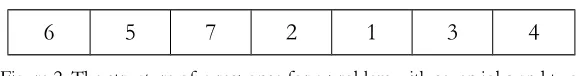
A limited number of weeds, called pop size, is randomly produced and considered as the initial population. In addition, the values of two fitness functions of each weed are calculated as soon as it is generated. In this study, the two fitness functions are the minimization of make span and the minimization of average tardiness. The weed structure is shown in Figure 2.
Each response (country) is an array of 1 × N integers, where N shows the number of jobs. Each array
6 5 7 2 1 3 4
Figure 2. The structure of a response for a problem with seven jobs and two machines in the first station and three machines in the second station
3.2. Fuzzy Dominance Based Sorting
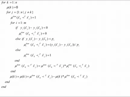
The first step of fuzzy dominance sorting in the DMOIWO is to compute the fuzzy dominances of the weeds in the population. The weeds are then sorted by fuzzy dominance in ascending order. The structure of the fuzzy dominance calculation is shown in Figure 3.
The first step for sorting based on fuzzy dominance in the proposed algorithm is the calculation of the fuzzy dominance of responses in the population. The responses are then sorted based on fuzzy dominance in ascending order. This approach is exactly opposite of sorting the responses based on crowding distance. After sorting the responses based on fuzzy dominance, the undefeated responses are stored in the archive. Pseudo-code algorithm, which is used for the calculation of the fuzzy dominance of each response, has been shown in figure 3. According to Figure 3, xi and xk are two responses, these two
responses either both defeat each other or neither one defeats the other in conventional multi-objective algorithm. However, the concept of the possibility of one defeating the other does not exist in the algorithms. In fact, in conventional multi-objective algorithms, there is zero or one state and an intermediate state does not make sense. Fuzzy dominance approach covers this concept as well. To understand the concept of fuzzy dominance approach, four definitions must be first given:
Definition 1: Suppose that the minimization problem consists of m objective functions ( yi = 1, 2, 3, …, m).
The answer, which includes a collection of possible responses, is shown by P Rm, where m is the
dimension of the problem.
Definition 2 (i th fuzzy dominance by one response):i {1, 2, 3, …, m} and μ
idom = yi(P) → [0,1] show
the monotonous non-decreasing membership. If yi( ) yi( ), P response is called the i th dominate
response on P. This relationship may also be shown by iF . If iF , the i th degree of the
defeated response equals μidom = ( yi( ) – yi( )) ≡ μidom ( iF ). Fuzzy dominance can be shown as iF
Definition 3 (fuzzy dominance by one response): P response is called the fuzzy response defeating P. If and only if i {1, 2, 3, …, n} for each i, the relationship iF exists, which is
shown by F ). If F ), the μ
idom ( F ) fuzzy dominance is obtained by calculating iF
fuzzy share relations for each response i. Fuzzy share operator is shown by using one of t-form family relationships:
(1)
Consider SA response population. A Definition 4 (fuzzy dominance in the population): response P
is said to be defeated in S from fuzzy view point of view if the fuzzy dominance is performed by any other
P response. Thus, fuzzy dominance can be performed by union operator as follows:
(2)
The pseudo-code algorithm used to calculate fuzzy dominance is as follows.
In this model, n solutions are assumed and for each of these solutions μ(k) k {1, 2, …, n}, i.e. a membership function, is calculated. To calculate μ(k), based on the objective function values, a mutual comparison between the kth solution and all the other solutions are made and μ(k) is updated accordingly.
If for the ith objective function y
i( j) – yi( k) 0, then μ(k) is set to zero, but if yi( j) – yi( k) pi, in
which pi is a positive number that shows the difference between maximum and minimum value of the
fitness function, μ(k) is updated based on, otherwise μ(k) will be set to one.
Finally, after calculating fuzzy dominance, the fuzzy responses are sorted in ascending order based on membership function.
3.3. Reproduction
Every seed grows to become a new plant (Weed). These weeds then produce other seeds with respect to their fitness function. The maximum possible seed (Smax) will be produced by the weed with minimum fitness function and the minimum possible seed (Smin) will be generated by the weed with maximum fitness function. The number of seeds, which is produced by other weeds, is obtained using a linear function varying in a range between Smin and Smax and is dependent on the value of these fitness functions. Figure 4 depicts the relationship between the number of seeds and value of fitness function.
Figure 4. relationship between the number of seed and value of fitness function (Mehrabian and Lucas, 2006)
For this purpose, the sigma value of each iteration is obtained in the first of each iteration as follows:
Where itermax is the maximum number of iterations and iter is the current iteration. In addition, σinitial and
σfinal are the initial sigma and the final sigma, respectively. n is the non-linear modulation index. The value
of σfinal is equal to two and the value of σinitial is equal to the percent of job numbers (η) obtained as
follows:
(4)
The number of weeds in each repetition is equal to parameter “PopSize”. Weeds had been sorted based on fuzzy dominance in the previous step.
Each weed generates some seeds based on its rank in the population. The number of seeds, which are generated by each weed, is obtained using the following equation.
(5)
The maximum possible and minimum possible seeds, which are produced by one weed, are shown by
parameters “Smax” and “Smin”, respectively. In this algorithm, ranki shows the rank of ith weed. Smin
has been assumed zero in this algorithm.
When the number of seeds generated by each weed is determined, the seeds of each weed are produced according to the following process: Having produced the job sequences in the weed’s array, as shown in
Figure 4, a number in the range of 2 and σiter is randomly generated, which is named nmove, nmove
positions are then randomly selected from the given weed. Afterwards, the sequence of these positions is changed randomly.
This producer is carried out for an example with seven jobs. Assume that nmove is equal to 3 and the selected jobs are 2, 7 and 5 (see Figure 5). In addition, the random sequence for these jobs is 5, 7 and 2. Therefore, the mutated weed is depicted in Figure 6.
3 2 4 5 1 6 7
Figure 5. Given solution with three random selected positions
3 5 4 7 1 6 2
Notice that if the random number generated in the second step is equal to 2, exchange will be done to produce new seeds.
3.4. Mutation on the Weeds
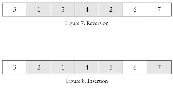
Humans have recently generated an entirely new category of very nasty weeds, which is called herbicide resistant weeds. The resistant weeds are produced by mutation of the initial weeds. Two operators including insertion and reversion are applied as mutation operators. Furthermore, this operation is done on the percent of population shown by pm each iteration. The structures of insertion and reversion operators are as follows: Having Figure 5, assuming that two jobs have been selected randomly (jobs 2 and 1).
3 1 5 4 2 6 7
Figure 7. Reversion
3 2 1 4 5 6 7
Figure 8. Insertion
Reversion: In this policy, the positions of selected jobs are exchanged. The jobs located in between the swapped jobs are then reversed, too (Figure 7).
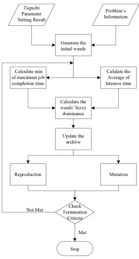
Figure 9. DMOIWO Flowchart
3.5. Competitive Exclusion
3.6. Archive Adaption
In each iteration, after competitive exclusion, the non-dominated solutions are selected and added to the archive. The fuzzy dominances of the archive members are then computed and the members are sorted by fuzzy dominance in ascending order. Afterwards, the stages including reproduction and mutation are carried out on the archive members. Finally, the non-dominated solutions are selected in the archive and the other solutions are removed. If the number of solutions in the archive is more than the archive size (nArchive), the solutions in archive are sorted based on crowding distance and then the number of the best archive solutions with size of “nArchive” is selected.
3.7. Stopping Criteria
The processes of weed generating are stopped when a fixed number of generations are satisfied. This is shown by parameter “MaxIt”. Figure 9 gives the DMOIWO in pseudo-code.
4. Criteria for Comparison of Multi-Objective Approaches
Four criteria are considered for the comparison of multi-objective approaches in this work:
• Diversification metric (DM): The spread of solution set is measured by this metric and calculated by:
(6)
• Mean ideal distance (MID): This metric is used to determine the closeness between Pareto solutions
and ideal point . MID is calculated by:
(7)
Where n is the number of non-dominated solutions and and are the maximum and
minimum values of each fitness function among all non-dominated solutions obtained by the algorithms, respectively. According to this definition, better performance belongs to the algorithm with the lowest value of the MID
(8)
• Quality metric (QM): For calculation of this algorithm, the non-dominated solutions obtained by the algorithms are first put together. Afterwards, the non-dominated solutions are chosen. Finally, the percentage of the non-dominated solutions belonging to each algorithm is obtained as QM (Tapkan et al., 2012).
5. Computational Experiments
In this section, firstly, the procedure for data generation and parameter setting approach is described, followed by the description of performance evaluation for proposed DMOIWO with NSGAII , PAES, and MOPSO. It is noticeable that all algorithms are implemented in MATLAB 2011a and run on a PC with 2.53 GHz Intel Core 2 Duo and 4 GB of RAM memory.
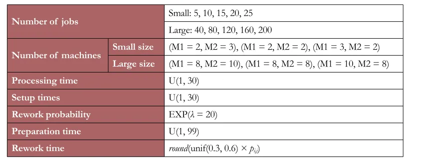
5.1. Simulation model parameters
Number of jobs Small: 5, 10, 15, 20, 25
Large: 40, 80, 120, 160, 200
Number of machines Small size (M1 = 2, M2 = 3), (M1 = 2, M2 = 2), (M1 = 3, M2 = 2) Large size (M1 = 8, M2 = 10), (M1 = 8, M2 = 8), (M1 = 10, M2 = 8)
Processing time U(1, 30)
Setup times U(1, 30)
Rework probability EXP(λ = 20)
Preparation time U(1, 99)
Rework time round(unif(0.3, 0.6) × pi,j)
Table 1. Parameters and their levels
5.2. Parameter Setting
Appropriate design of parameters and operators has a meaningful impact on the efficiency of the algorithms used. Taguchi parameter setting has been used for setting the parameters of the proposed algorithm. For this purpose, parameter setting has been performed for an algorithm for a particular problem consisting of 80 jobs, 8 machines in the first station and 10 in the second and the results are given below:
DMOIWO algorithm consists of 7 control factors including η, PopSize, nArchive, MaxIt, n, Smax, and
pMutation. In order to reduce the number of parameters, the product of MaxIt and PopSize has been considered here. Therefore, there will be 6 parameters. There are three levels for each factor shown in Table 2. In addition, each factor is represented by a symbol shown in Table 2.
Number Factors Symbol Level 1 Level 2 Level 3
1 (MaxIt, PopSize) A (250, 40) (200, 50) (100, 100)
2 N B 2 3 4
3 Smax C 8 10 12
4 η D 0.2 0.25 0.3
5 pMutation E 0.2 0.3 0.4
6 nArchive F 50 75 100
Table 2. Factors and their levels
The orthogonal array for this algorithm is L27. Table 3 shows L27 orthogonal array.
Trial A B C D E F
1 A(1) B(1) C(1) D(1) E(1) F(1)
2 A(1) B(1) C(1) D(1) E(2) F(2)
3 A(1) B(1) C(1) D(1) E(3) F(3)
4 A(1) B(2) C(2) D(2) E(1) F(1)
5 A(1) B(2) C(2) D(2) E(2) F(2)
6 A(1) B(2) C(2) D(2) E(3) F(3)
7 A(1) B(3) C(3) D(3) E(1) F(1)
8 A(1) B(3) C(3) D(3) E(2) F(2)
9 A(1) B(3) C(3) D(3) E(3) F(3)
10 A(2) B(1) C(2) D(3) E(1) F(2)
11 A(2) B(1) C(2) D(3) E(2) F(3)
12 A(2) B(1) C(2) D(3) E(3) F(1)
13 A(2) B(2) C(3) D(1) E(1) F(2)
14 A(2) B(2) C(3) D(1) E(2) F(3)
15 A(2) B(2) C(3) D(1) E(3) F(1)
16 A(2) B(3) C(1) D(2) E(1) F(2)
17 A(2) B(3) C(1) D(2) E(2) F(3)
18 A(2) B(3) C(1) D(2) E(3) F(1)
19 A(3) B(1) C(3) D(2) E(1) F(3)
20 A(3) B(1) C(3) D(2) E(2) F(1)
21 A(3) B(1) C(3) D(2) E(3) F(2)
22 A(3) B(2) C(1) D(3) E(1) F(3)
23 A(3) B(2) C(1) D(3) E(2) F(1)
24 A(3) B(2) C(1) D(3) E(3) F(2)
25 A(3) B(3) C(2) D(1) E(1) F(3)
26 A(3) B(3) C(2) D(1) E(2) F(1)
27 A(3) B(3) C(2) D(1) E(3) F(2)
Table 3. L27 orthogonal array for ICASA algorithm
Parameters Scales
Small Large
(MaxIt, Pop Size) (100,50) (200,50)
n 3 3
Smax 10 12
η 0.2 0.25
PMutation 0.3 0.3
nArchive 40 50
Table 4. Parameter setting values for the proposed DMOIWO algorithm
More data are shown in Figure 12 for further analysis. Considering the table, the factor with greater delta value has a greater impact on the algorithm. Thus, factor MaxIt, PopSize has the greatest impact on the algorithm, followed by η, PMutation, n, nArchive and Smax, respectively.
Figure 12. S/N values
5.3. Calculation Results
Problem Quality metric Diversity metrice RAS metric MID metric
No.
Jobs M1 × M2 DMOIWO PAES MOPSO NSGA-II DMOIWO PAES MOPSO NSGA-II DMOIWO PAES MOPSO NSGA-II DMOIWO PAES MOPSO NSGA-II
5
2 × 2 0.33 0 0.66 0 65.19 68.69 62.36 82.2 95.4 103.16 50.5 110.6 73.79 79.49 45.09 87.33 2 × 3 0.5 0 0.125 0.375 44.59 77.01 53.36 44.59 31.5 59 35 34.33 27.93 46.21 33.54 31.69 3 × 2 1 0 0 0 44.59 45.45 45.45 45.45 31.5 101 101 101 27.93 75.99 75.99 75.99
10
2 × 2 0 0 0 1 31.82 49.67 31.76 45.45 401.25 423.75 701.66 32 284.64 300.97 496.84 32 2 × 3 0 0.33 0 0.66 52.8 49.6 64.56 19.64 202.2 46.33 552.66 15 144.01 37.27 392.34 13.61 3 × 2 0.5 0.5 0 0 58.18 92.08 25.02 51.45 59.75 68 571 574 48.73 59.07 404.026 46.218
15
2 × 2 1 0 0 0 57.01 8.06 48.38 83.77 31.6 511.5 633.75 580.2 28.84 361.72 448.9 412.08 2 × 3 1 0 0 0 85.44 60.16 89.62 71.19 45 109.66 306 268.5 39.5 81.51 219.19 191.55 3 × 2 0 1 0 0 49.98 67.72 84 69.46 119.6 42 384 87.5 93.7 42 971.5 66.08
20
2 × 2 1 0 0 0 132.67 30.14 6.08 74.24 66.66 141.5 290.5 213 60.24 100.73 205.94 153.26 2 × 3 1 0 0 0 38.32 70.93 100.8 25 21.5 132.14 244 813 21.5 94.47 178.22 578.14
3 × 2 1 0 0 0 14.56 220 233 25 9 194 179 440 9 137.29 126.62 327.24
25
2 × 2 1 0 0 0 39.92 55.03 48.01 259 19 452.5 498.5 363 18.3 323.3 353.05 257.19 2 × 3 1 0 0 0 43.41 66.27 76.24 112.29 28.3 176.3 271.6 485 26.88 127.35 194.03 345.93
3 × 2 1 0 0 0 36.4 265 255 321 22.4 73 245 181 20.49 53 147.3 130.9
Table 5. Calculation results
Problem Quality metric Divercity metrice RAS metric MID metric
No. Jobs M1 × M2 DMOIWO PAES MOPSO NSGA-II DMOIWO PAES MOPSO NSGA-II DMOIWO PAES MOPSO NSGA-II DMOIWO PAES MOPSO NSGA-II
40
16 × 20 1 0 0 0 75.43 107.61 74.8 86.3 38.57 105.11 122.8 113.33 34.76 84.35 92.94 88.26 20 × 20 1 0 0 0 40.16 90.33 55.07 37.94 32.25 110 84.3 51 28.29 81.7 62.24 37.63 24 × 20 0.4 0.2 0 0.4 30.46 47.12 89.35 98.27 23 41.15 103.2 42 19.82 34.5 78.8 37.2
80
16 × 20 1 0 0 0 64.32 79.81 117.2 101.39 33.2 121.75 157.42 99.44 32.08 88.8 116.4 77.9 20 × 20 1 0 0 0 52.92 61.71 54.4 83.09 30.66 153.25 153 111.83 27.72 111.45 111.73 86.54 24 × 20 0.625 0.2 0 0.375 77.89 49.93 55.8 43.86 50.77 124.5 166.4 34 44.54 89.63 119.01 30.27
120
16 × 20 1 0 0 0 64.07 90.6 63.9 59.54 41.75 152.45 153 79.66 41.66 121.12 131.12 105.24 20 × 20 0.8 0 0 0.2 104.34 42.059 150.01 120.8 70.5 105.5 155.92 77.4 64.85 79.55 117.91 62.51 24 × 20 1 0 0 0 85.58 46.01 74.88 713.7 50.75 166.2 180.8 140.14 37.27 111.31 112.08 62.38
160
16 × 20 1 0 0 0 76.94 124.08 102.48 72.89 41 143.2 173.5 68.2 38.59 108.16 126.8 61.15 20 × 20 1 0 0 0 68.014 122.3 65.29 111.01 43.11 195.2 167.5 132.5 35.89 144.37 122.19 100.1 24 × 20 0.83 0 0 0.16 69.02 70.4 59.77 75.8 38.4 97.33 109.66 64.4 35.17 72.97 80.47 53.45
200
16 × 20 1 0 0 0 100.64 44.1 121.65 128.84 56.75 187.33 230.83 183.66 46.48 124.69 132.08 89.22 20 × 20 1 0 0 0 87.81 144.6 87.8 83.4 47.6 168.14 179.8 118.5 52.09 135.55 170.83 136.63 24 × 20 1 0 0 0 64.51 82.32 110.38 46.75 43.66 142.6 173.33 112.66 37.63 104.43 129.6 81.97
6. Conclusion
NWTSFFS problem has been investigated given the machinery start-up time, preparation of jobs, rework probability and non-identical machinery constraints considering minimization of maximum completion and average lateness times simultaneously in a multi-objective manner in this work. The problem was then solved using the proposed DMOIWO and conventional NSGA-II, PAES and MOPSO algorithms. Ultimately, indices including DM, RAS, MID and QM were presented in order to compare the efficiency of the algorithms. The results of the comparison indicated the efficiency of DMOIWO algorithm. Although the proposed algorithm is efficient in term of quality of the obtained solutions, finding appropriate parameters to reach a high-quality solution needs more endeavor and is a time-consuming process. In this work, Taguchi parameter setting was used to solve this problem, as a feature work it would be worthwhile to enhance the algorithm such that it can set its parameters based on the convergence rate and quality of the best solution. Furthermore, by increasing the number of decision variables the size of the solution space grows exponentially. In these cases, it would be beneficial to exploit a heuristic algorithm to generate some initial solutions that have acceptable level of quality. This hybrid algorithm can decrease the running time and the number of iterations as well.
References
Abdollahpour, S., & Rezaian, J. (2016). Two new meta-heuristics for no-wait flexible flow shop scheduling
problem with capacitated machines, mixed make-to-order and make-to-stock policy. Soft Computing, 1-19.
Aldowaisan, T. (2001). A new heuristic and dominance relations for no-wait flowshops with setups.
Computers & Operations Research, 28(6), 563-584. https://doi.org/10.1016/S0305-0548(99)00136-7
Aldowaisan, T., & Allahverdi, A. (1998). Total flowtime in no-wait flowshops with separated setup times.
Computers & Operations Research, 25(9), 757-765. https://doi.org/10.1016/S0305-0548(98)00002-1
Aldowaisan, T., & Allahverdi, A. (2004). New heuristics for m-machine no-wait flowshop to minimize total completion time. Omega, 32(5), 345-352. https://doi.org/10.1016/j.omega.2004.01.004
Allahverdi, A., & Aldowaisan, T. (2002). No-wait flowshops with bicriteria of makespan and total completion time. Journal of the Operational Research Society, 53(9), 1004-1015.
Allahverdi, A., & Aldowaisan, T. (2004). No-wait flowshops with bicriteria of makespan and maximum lateness. European Journal of Operational Research, 152(1), 132-147. https://doi.org/10.1016/S0377-2217(02)00646-X
Bonney, M., & Gundry, S. (1976). Solutions to the constrained flowshop sequencing problem. Journal of the Operational Research Society, 27(4), 869-883. https://doi.org/10.1057/jors.1976.176
Callahan, J. R. (1972). The nothing hot delay problem in the production of steel. Thesis. Department of Industrial Engineering, University of Toronto, Canada.
Chang, J., Yan, W., & Shao, H. (2004). Scheduling a two-stage no-wait hybrid flowshop with separated setup and removal times. Paper presented at the American Control Conference.
Davendra, D., Zelinka, I., Bialic-Davendra, M., Senkerik, R., & Jasek, R. (2013). Discrete self-organising migrating algorithm for flow-shop scheduling with no-wait makespan. Mathematical and Computer Modelling, 57(1), 100-110. https://doi.org/10.1016/j.mcm.2011.05.029
Elyasi, M., Jafarzadeh, H., & Khoshalhan, F. (2012). An economical order quantity model for items with
imperfect quality: A non-cooperative dynamic game theoretical model. Paper presented at the 3rd
International Logistics and Supply chain Conference.
Framinan, J. M., & Nagano, M. S. (2008). Evaluating the performance for makespan minimisation in no-wait flowshop sequencing. Journal of materials processing technology, 197(1), 1-9.
https://doi.org/10.1016/j.jmatprotec.2007.07.039
Gao, K.-Z, Pan, Q.-k., & Li, J.-Q. (2011). Discrete harmony search algorithm for the no-wait flow shop scheduling problem with total flow time criterion. The International Journal of Advanced Manufacturing Technology, 56(5-8), 683-692. https://doi.org/10.1007/s00170-011-3197-6
Gerami, A., Allaire, P., & Fittro, R. (2015). Control of Magnetic Bearing With Material Saturation Nonlinearity. Journal of Dynamic Systems, Measurement, and Control, 137(6), 061002.
https://doi.org/10.1115/1.4029125
Gilmore, P.C., & Gomory, R.E. (1964). Sequencing a one state-variable machine: A solvable case of the traveling salesman problem. Operations Research, 12(5), 655-679. https://doi.org/10.1287/opre.12.5.655
Goyal, S., & Sriskandarajah, C. (1988). No-wait shop scheduling: computational complexity and approximate algorithms. Opsearch, 25(4), 220-244.
Gupta, J.N. (1976). Optimal flowshop schedules with no intermediate storage space. Naval Research Logistics Quarterly, 23(2), 235-243. https://doi.org/10.1002/nav.3800230206
Gupta, J.N., Strusevich, V.A., & Zwaneveld, C.M. (1997). Two-stage no-wait scheduling models with setup
and removal times separated. Computers & Operations Research, 24(11), 1025-1031.
https://doi.org/10.1016/S0305-0548(97)00018-X
Hall, N.G., & Sriskandarajah, C. (1996). A survey of machine scheduling problems with blocking and no-wait in process. Operations research, 44(3), 510-525. https://doi.org/10.1287/opre.44.3.510
Haouari, M., Hidri, L., & Gharbi, A. (2006). Optimal scheduling of a two-stage hybrid flow shop.
Mathematical Methods of Operations Research, 64(1), 107-124. https://doi.org/10.1007/s00186-006-0066-4
Hasani, R., Jafarzadeh, H., & Khoshalhan, F. (2013). A new method for supply chain coordination with
credit option contract and customers’ backordered demand. Uncertain Supply Chain Management, 1(4),
207-218. https://doi.org/10.5267/j.uscm.2013.09.002
Hmida, A.B., Haouari, M., Huguet, M.-J., & Lopez, P. (2011). Solving two-stage hybrid flow shop using climbing depth-bounded discrepancy search. Computers & Industrial Engineering, 60(2), 320-327. https://doi.org/10.1016/j.cie.2010.11.015
Huang, R.-H., Yang, C.-L., & Huang, Y.-C. (2009). No-wait two-stage multiprocessor flow shop scheduling with unit setup. The International Journal of Advanced Manufacturing Technology, 44(9-10), 921-927. https://doi.org/10.1007/s00170-008-1865-y
Jafarzadeh, H., Gholami, S., & Bashirzadeh, R. (2014). A new effective algorithm for on-line robot motion planning. Decision Science Letters, 3(1), 121-130. https://doi.org/10.5267/j.dsl.2013.07.004
Jafarzadeh, H., Moradinasab, N., Eskandari, H. & Gholami, S. (2017). Genetic Algorithm for A Generic Model of Reverse Logistics Network. International Journal of Engineering Innovation & Research, 6(4), 174-178.
Jolai, F., Asefi, H., Rabiee, M., & Ramezani, P. (2013). Bi-objective simulated annealing approaches for no-wait two-stage flexible flow shop scheduling problem. Scientia Iranica, 20(3), 861-872.
Jolai, F., Sheikh, S., Rabbani, M., & Karimi, B. (2009). A genetic algorithm for solving no-wait flexible flow lines with due window and job rejection. The International Journal of Advanced Manufacturing Technology,
42(5), 523-532. https://doi.org/10.1007/s00170-008-1618-y
Kalczynski, P.J., & Kamburowski, J. (2007). On no-wait and no-idle flow shops with makespan criterion.
King, J., & Spachis, A. (1980). Heuristics for flow-shop scheduling. International Journal of Production Research, 18(3), 345-357. https://doi.org/10.1080/00207548008919673
Kundu, D., Suresh, K., Ghosh, S., Das, S., Panigrahi, B.K., & Das, S. (2011). Multi-objective optimization with artificial weed colonies. Information Sciences, 181(12), 2441-2454. https://doi.org/10.1016/j.ins.2010.09.026 Kurian, K. (1987). Scheduling of Batch Processes. PhD. Purdue University, West Lafayette, Indiana.
Kuriyan, K., & Reklaitis, G. (1985). Approximate scheduling algorithms for network flowshops. Paper presented at the The Institute of Chemical Engineers, Symposium Series.
Levner, E. (1969). Optimal planning of parts machining on a number of machines. Automation and Remote
Control, 12, 1972-1981.
Liu, Y., & Feng, Z. (2014). Two-machine no-wait flowshop scheduling with learning effect and convex resource-dependent processing times. Computers & Industrial Engineering, 75, 170-175.
https://doi.org/10.1016/j.cie.2014.06.017
Liu, Z., Xie, J., Li, J., & Dong, J. (2003). A heuristic for two-stage no-wait hybrid flowshop scheduling with a single machine in either stage. Tsinghua Science and Technology, 8(1), 43-48.
Marinakis, Y., Migdalas, A., & Pardalos, P.M. (2008). Expanding neighborhood search–GRASP for the probabilistic traveling salesman problem. Optimization Letters, 2(3), 351-361. https://doi.org/10.1007/s11590-007-0064-3
Mehrabian, A.R., & Lucas, C. (2006). A novel numerical optimization algorithm inspired from weed colonization. Ecological Informatics, 1(4), 355-366. https://doi.org/10.1016/j.ecoinf.2006.07.003
Moradinasab, N., Shafaei, R., Rabiee, M., & Ramezani, P. (2013). No-wait two stage hybrid flow shop scheduling with genetic and adaptive imperialist competitive algorithms. Journal of Experimental & Theoretical Artificial Intelligence, 25(2), 207-225. https://doi.org/10.1080/0952813X.2012.682752
Moradinasab, N., Shafaei, R., Rabiee, M., & Mazinani, M. (2012). Minimization of maximum tardiness in a no-wait two stage flexible flow shop. International Journal of Artificial Intelligence, 8(S12), 166-181.
Pan, Q.-K., Tasgetiren, M.F., & Liang, Y.-C. (2008). A discrete particle swarm optimization algorithm for the no-wait flowshop scheduling problem. Computers & Operations Research, 35(9), 2807-2839.
Pan, Q.-K., Wang, L., & Qian, B. (2009). A novel differential evolution algorithm for bi-criteria no-wait flow shop scheduling problems. Computers & Operations Research, 36(8), 2498-2511.
https://doi.org/10.1016/j.cor.2008.10.008
Pang, K.-W. (2013). A genetic algorithm based heuristic for two machine no-wait flowshop scheduling
problems with class setup times that minimizes maximum lateness. International Journal of Production
Economics, 141(1), 127-136. https://doi.org/10.1016/j.ijpe.2012.06.017
Papadimitriou, C.H., & Kanellakis, P.C. (1984). On concurrency control by multiple versions. ACM
Transactions on Database Systems (TODS), 9(1), 89-99. https://doi.org/10.1145/348.318588
Qian, B., Wang, L., Hu, R., Huang, D., & Wang, X. (2009). A DE-based approach to no-wait flow-shop scheduling. Computers & Industrial Engineering, 57(3), 787-805. https://doi.org/10.1016/j.cie.2009.02.006
Raaymakers, W.H., & Hoogeveen, J. (2000). Scheduling multipurpose batch process industries with no-wait restrictions by simulated annealing. European Journal of Operational Research, 126(1), 131-151. https://doi.org/10.1016/S0377-2217(99)00285-4
Rajendran, C. (1994). A no-wait flowshop scheduling heuristic to minimize makespan. Journal of the
Operational Research Society, 45(4), 472-478. https://doi.org/10.1057/jors.1994.65
Ramezani, P., Rabiee, M., & Jolai, F. (2015). No-wait flexible flowshop with uniform parallel machines and sequence-dependent setup time: a hybrid meta-heuristic approach. Journal of Intelligent Manufacturing,
26(4), 731-744. https://doi.org/10.1007/s10845-013-0830-2
Ramudhin, A., & Ratliff, H. D. (1995). Generating daily production schedules in process industries. IIE Transactions, 27(5), 646-657.
Reddi, S., & Ramamoorthy, C. (1972). On the Flow-Shop Sequencing Problem with No Wait in Process.
Journal of the Operational Research Society, 23(3), 323-331. https://doi.org/10.1057/jors.1972.52
Salvador, M.S. (1973). A solution to a special class of flow shop scheduling problems. Paper presented at the Symposium on the Theory of Scheduling and its Applications. https://doi.org/10.1007/978-3-642-80784-8_7 Sang, H.-Y., Duan, P.-Y., &Li, J.-Q. (2016). A Discrete Invasive Weed Optimization Algorithm for the
No-Wait Lot-Streaming Flow Shop Scheduling Problems. International Conference on Intelligent Computing. Springer International Publishing, 2016.
Sidney, J.B., Potts, C.N., & Sriskandarajah, C. (2000). A heuristic for scheduling two-machine no-wait flow shops with anticipatory setups. Operations Research Letters, 26(4), 165-173. https://doi.org/10.1016/S0167-6377(00)00019-5
Sriskandarajah, C. (1993). Performance of scheduling algorithms for no-wait flowshops with parallel machines. European Journal of Operational Research, 70(3), 365-378. https://doi.org/10.1016/0377-2217(93)90248-L
Sriskandarajah, C., & Ladet, P. (1986). Some no-wait shops scheduling problems: complexity aspect.
European journal of operational research, 24(3), 424-438. https://doi.org/10.1016/0377-2217(86)90036-6
Su, L.-H., & Lee, Y.-Y. (2008). The two-machine flowshop no-wait scheduling problem with a single server to minimize the total completion time. Computers & Operations Research, 35(9), 2952-2963. https://doi.org/10.1016/j.cor.2007.01.002
Tapkan, P., Özbakır, L., & Baykasoğlu, A. (2012). Bees algorithm for constrained fuzzy multi-objective two-sided assembly line balancing problem. Optimization Letters, 6(6), 1039-1049.
https://doi.org/10.1007/s11590-011-0344-9
Tavakkoli-Moghaddam, R., Rahimi-Vahed, A., & Mirzaei, A.H. (2007). A hybrid multi-objective immune algorithm for a flow shop scheduling problem with bi-objectives: weighted mean completion time and weighted mean tardiness. Information Sciences, 177(22), 5072-5090. https://doi.org/10.1016/j.ins.2007.06.001 Thornton, H.W., & Hunsucker, J.L. (2004). A new heuristic for minimal makespan in flow shops with
multiple processors and no intermediate storage. European Journal of Operational Research, 152(1), 96-114. https://doi.org/10.1016/S0377-2217(02)00524-6
Tseng, L.-Y., & Lin, Y.-T. (2010). A hybrid genetic algorithm for no-wait flowshop scheduling problem.
International Journal of Production Economics, 128(1), 144-152. https://doi.org/10.1016/j.ijpe.2010.06.006
Van Deman, J.M., & Baker, K.R. (1974). Minimizing mean flowtime in the flow shop with no intermediate queues. AIIE Transactions, 6(1), 28-34. https://doi.org/10.1080/05695557408974929
Wang, C., Li, X., & Wang, Q. (2010). Accelerated tabu search for no-wait flowshop scheduling problem with maximum lateness criterion. European Journal of Operational Research, 206(1), 64-72.
https://doi.org/10.1016/j.ejor.2010.02.014
Wang, Z., Xing, W., & Bai, F. (2005). No-wait flexible flowshop scheduling with no-idle machines.
Operations Research Letters, 33(6), 609-614. https://doi.org/10.1016/j.orl.2004.10.004
Wismer, D. (1972). Solution of the flowshop-scheduling problem with no intermediate queues. Operations
research, 20(3), 689-697. https://doi.org/10.1287/opre.20.3.689
Xie, J., & Wang, X. (2005). Complexity and algorithms for two-stage flexible flowshop scheduling with availability constraints. Computers & Mathematics with Applications, 50(10), 1629-1638.
https://doi.org/10.1016/j.camwa.2005.07.008
Journal of Industrial Engineering and Management, 2017 (www.jiem.org)
Article’s contents are provided on an Attribution-Non Commercial 3.0 Creative commons license. Readers are allowed to copy, distribute and communicate article’s contents, provided the author’s and Journal of Industrial Engineering and Management’s