Identifying Twitter Spam by Utilizing Random Forests

Scholarly Horizons: University of Minnesota, Morris

Undergraduate Journal

Volume 4 | Issue 2

Article 5

July 2017

Identifying Twitter Spam by Utilizing Random

Forests

Humza S. Haider

University of Minnesota, Morris

Follow this and additional works at:

http://digitalcommons.morris.umn.edu/horizons

Part of the

Computer Sciences Commons

This Article is brought to you for free and open access by University of Minnesota Morris Digital Well. It has been accepted for inclusion in Scholarly Horizons: University of Minnesota, Morris Undergraduate Journal by an authorized editor of University of Minnesota Morris Digital Well. For more information, please [email protected].

Recommended Citation

Haider, Humza S. (2017) "Identifying Twitter Spam by Utilizing Random Forests,"Scholarly Horizons: University of Minnesota, Morris Undergraduate Journal: Vol. 4 : Iss. 2 , Article 5.

Cover Page Footnote

This work is licensed under the Creative Commons Attribution- NonCommercial-ShareAlike 4.0

Identifying Twitter Spam by Utilizing Random Forests

Humza S. Haider

Division of Science and Mathematics University of Minnesota, Morris Morris, Minnesota, USA 56267

[email protected]

ABSTRACT

The use of Twitter has rapidly grown since the first tweet in 2006. The number of spammers on Twitter shows a similar increase. Classifying users into spammers and non-spammers has been heavily researched, and new methods for spam detection are developing rapidly. One of these classifi-cation techniques is known as random forests. We examine three studies that employ random forests using user based features, geo-tagged features, and time dependent features. Each study showed high accuracy rates and F-measures with the exception of one model that had a test set with a more realistic proportion of spam relative to typical testing proce-dures. These studies suggest that random forests, in combi-nation with unique feature selection can be used to identify spam and spammers with high accuracy but may have short-comings when applied to real world situations.

Keywords

random forests,decision trees, spam, machine learning

1.

INTRODUCTION

Twitter has become one of the most widely used social media services across the world averaging roughly 500 mil-lion tweets per day [6]. As a result, the number of malicious users on Twitter has also expanded. On Twitter, spam is defined as any unsolicited, repeated actions that negatively impact other users. On Twitter, spam can manifest itself as links to harmful websites (such as phishing or malware websites) or distribution of pornographic materials.

The data used to identify spam tweets and spammers is made up offeaturesalso known asvariables. Features are a way of categorizing a dataset into mutually exclusive groups such as tweets into spam and not spam or users into spam-mers and non-spamspam-mers. Another feature could be an indi-cator of whether or not a user has reported a tweet as spam. This feature,Reported, takes on the values Reported= yes andReported= no. Note that a reported tweet doesn’t im-ply the tweet is spam, just that it has been reported. All features in this paper are denoted with italics.

Spammers typically share traits within their tweets and their accounts. For example, in order to draw more atten-tion to their tweets, a spammer is likely to have tweets

con-This work is licensed under the Creative Commons Attribution-NonCommercial-ShareAlike 4.0 International License. To view a copy of this license, visit http://creativecommons.org/licenses/by-nc-sa/4.0/.

UMM CSci Senior Seminar Conference, April 2017Morris, MN.

taining manymentions, a way of bringing a user’s attention to a tweet. Specifically, if we sawNumber of Mentions = 5, it would imply the spammer mentioned 5 other users in their tweet. If a user has many mentions across their tweets the likelihood that they are a spammer increases. By combin-ing multiple features, models can be constructed to identify spammers and spam tweets with a high degree of accuracy. Machine learning is a specific type of artificial intelligence that allows computers to learn without being specifically programmed. Techniques in the field range from classifica-tion analysis to pattern recogniclassifica-tion. Our paper explores the machine learning technique known asrandom forests. Intro-duced in 2001 by Leo Breiman, random forests have become one of the most widely used methods for classification analy-sis. We examine three papers which are similar in that each use a random forest to identify either spam or spammers on Twitter but are different in their feature selection.

Authors, Chen et al., [2] use features directly available from a tweet itself and features tied to a user’s account. For example, they identify the the number of hashtags in a tweet and then also examine the number of followers that the user has. Guo and Chen [3] use similar features, but also in-clude geographical information tied to a user and the user’s tweets. For example, if a user travels large distances in rela-tively short periods between tweets they may be a spammer. Lastly, Washha et al. [6] make use of time-dependent fea-tures to identify spammers. One such feature is how tweet-ing diversity may change over time. If a user has little-to-no diversity in their tweets, they are likely tweeting a single message many times, making them a spammer.

First, a discussion of the concept and details of a random forest is given in Section 2. From there, the three studies’ features are presented in Section 3. In Section 4, the analysis of each study will be presented and a comparison of the analyses will be made. Lastly, concluding remarks can be found in Section 5.

2.

BACKGROUND

Before we begin to discuss the intricacies of a random forest, we will first consider a single tree. Random forests are constructed from a combination of decision trees. A decision tree is a method of classifying a feature of interest, denotedT, through the use of other features available. In the case of detecting spam tweets, knowing whether a URL is present in a tweet, the users account age, and if the tweet has been reported as spam could all be assessed before deciding on whether a tweet is spam or not spam. Table 1 gives examples of these features.

1

Haider: Identifying Twitter Spam by Utilizing Random Forests

The data in Table 1 have been artificially constructed for the example and do not come from a real data set. Table 1 includes five features in total:U RL,AccountAge,Reported, the feature of interest (Class), and an identification feature (ID). TheIDfeature lets us uniquely identify rows, where each row serves as a single observation (tweet). The fea-tureU RLidentifies whether or not a URL is present in a tweet, AccountAge specifies whether an account is old or new, Reported specifies if the tweet has been reported as spam or not, andClassdetermines whether or not the tweet is spam.

Table 1: Example data for classifying a tweet as spam or not spam.

ID URL Account Age Reported Class

e1 No Old Yes Not Spam

e2 Yes Old Yes Not Spam

e3 No New Yes Spam

e4 No Old Yes Spam

e5 No New No Not Spam

e6 Yes New Yes Spam

e7 Yes New No Not Spam

e8 No Old No Non Spam

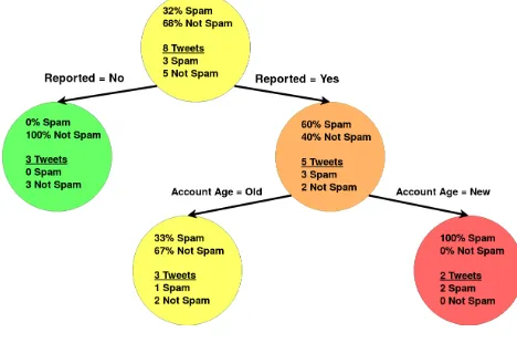
Using the data in Table 1 a decision tree has been con-structed, as seen in Figure 1. Each of the circles in the de-cision tree is referred to as anode. Within each node of the tree are the counts and proportions of Spam and Not Spam,

e.g. the topmost node contains 8 tweets, 3 Spam and 5 Not Spam, giving the proportions 32% Spam and 68% Not Spam. For each split of a node, the observations (rows) from Table 1 are partitioned. For example, in the left most node, which representsReported= No, the observations e5, e7, ande8

have been partitioned from the original dataset into a sub-set. This subset has the classifications 0% Spam and 100% Not Spam since each observation hasClass= Not Spam. In a given node, the classification with the higher proportion is theclassification decision of the observations within the node. Thus, for the observations in the leftmost node the classification decision is Not Spam.

Figure 1: Sample decision tree using data from Table 1.

2.1

Decision Trees

The goal of a decision tree is to recursively partition the observations from a dataset until the feature of interest,T, can be classified with maximum probability. We examine how splits in the nodes, as seen in Figure 1, are decided.

Suppose that each observation is labeled asposornegby

T. In Table 1, T is the Class feature andpos would refer

to Spam and neg to Not Spam. We then want to quantify the average information content of each observation when it is labeled as posor neg. Denoteppos as the proportion of

observations that are labeled asposbyT.

Suppose that ppos = 1, i.e. every tweet is spam. Then,

if we take a random observation and see thatT =pos, we haven’t learned anything new about the observation. This is because every observation will have T = pos; thus by looking at label given by T, no new information about the observation is learned. In the case thatppos= 1 we say the

average information content of the observations is 0 sinceT

doesn’t provide information about the observations. Alternatively, ifppos= 0.5 thenposandnegobservations

have the same probability of occurrence. Now, if we take a randomly drawn observation and see thatT=poswe know information about that specific observation since not all ob-servations have T = pos. Additionally, as ppos decreases

and we see an observation withT =posthe information in-creases because the observation is more unique than others among all observations. The standard way to quantify the average information content of theposobservations is:

Ipos=−log2ppos. (1)

The negative sign compensates for the fact that logarithm will always be negative since ppos ∈[0,1]. Additionally, as

ppos decreases, the quantity of information increase.

However, there are also observations with T =neg. In order to calculate the average information contents ofT we must consider bothposandneg observations. To compute this, we introduce entropy [5]. Entropy is calculated as

H(T) =−pposlog2ppos−pneglog2pneg. (2)

Note that H(T) becomes maximized at 1, namely when

ppos = pneg = 0.5. Further, entropy reaches a minimum

when either ppos = 1 orpneg = 1. When eitherppos = 1

or pneg = 1 it is known as perfect regularity since all

ob-servations have the same label ofT. Alternatively, ifppos=

pneg= 0.5 it is known as atotal lack of regularity.

Given the data in Table 1, we can calculateH(Class) as

H(Class) =−3

8log2

3 8

−5

8log2

5 8

= 0.954.

Note that since H(Class) is close to 1 there is a lack of regularity.

Decision trees were invented to deal with a lack of regu-larity. Given data with a lack of regularity, we use features which contribute the most information to classifying the la-bel of T. These features are used to partition the dataset into subsets with increased regularity. For example, of the features from Table 1 (excluding ID and Class) we want to identify which feature can best classify observations into

Class= Spam andClass= Not Spam.

We will denote a feature of the dataset asX. Note thatX

will partitionT into subsets,Ti, for each of the values that

X can take. For our case, whereT =Class, suppose X =

Account Ageand recall thatAccount Agecan take the values Old or New. In this case, Classwould be partitioned into

ClassOld={e1, e2, e4, e8}andClassNew={e3, e5, e6, e7}.

Let the number of elements inside ofTibe denoted as|Ti|.

Then, the probability that a randomly drawn observation from the dataset be contained inTi is

Pi=

|Ti|

Then, to calculate the entropy ofT given the values ofX

we can sum across the entropies of allTi, weighted by the

respectivePi. The equation for this is given by the following:

H(T|X) =X

i

Pi·H(Ti). (3)

H(T|X) gives the entropy of a system where the labels of

T, (pos,neg), and the values ofX are known. Specifically, this will tell us the regularity of T when the values of X

have been accounted for. Recall that we are trying to take a system with a lack of regularity and make it more regular so lower values ofH(T|X) are better.

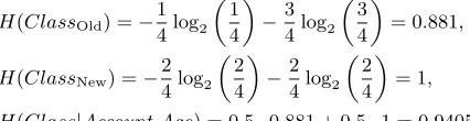
We will continue our example with AccountAge. Using the data in Table 1,|ClassOld|=|ClassNew|= 4. Thus, we

getPOld=PN ew= 0.5. To calculateH(Class|Account Age)

we make the following computations:

H(ClassOld) =−

1 4log2

1 4

−3

4log2

3 4

= 0.881,

H(ClassNew) =−

2 4log2

2 4

−2

4log2

2 4

= 1, H(Class|Account Age) = 0.5·0.881 + 0.5·1 = 0.9405.

Thus the entropy when both theClasslabel and the values forAccount Ageare known is 0.9405.

We then identify which feature supplies the most informa-tion about how to classify an observainforma-tion intopos or neg. This is known as the information gain from each feature. Continuing to denote a feature as X, information gain is realized as the difference between the entropy (regularity)

beforeX has been taken into account andafter X has been taken into account,i.e.

I(T|X) =H(T)−H(T|X). (4) ForAccountAgethis is:

I(Class|Account Age) =H(Class)−H(Class|Account Age) = 0.954−0.9405 = 0.014.

Then, by applying this same process to each feature, we can find which feature gives the most information about clas-sifying the labels ofClassand thus serves as the best choice to split on within a decision tree.

Using Equation (3) we find that

H(Class|URL) = 0.9511, H(Class|Reported) = 0.607.

Lastly, Equation (4) gives us the following:

I(Class|URL) =H(Class)−H(Class|URL) = 0.954−0.9511 = 0.003,

I(Class|Reported) =H(Class)−H(Class|Reported) = 0.954−0.607 = 0.347.

Thus we conclude that the maximum amount of information is contributed by the Reported feature. Looking back at Figure 1, we see that this indeed was the first feature split on. We will then apply the same process on the 5 tweets on the right node after the split, but stop on the left node since there is perfect regularity,i.e. all the observation have the sameClass value. In general, decision trees recursively apply this process to each node until either perfect regularity is attained or partitions fail to decrease the lack of regularity.

The procedure given above assumes all features have dis-crete values, i.e. the feature can be broken up into cat-egories. Unfortunately, this does not match many sets of realistic data; many features,e.g. the time interval between two consecutive tweets, takecontinuous values. A continu-ous feature is one that can take an infinite number of values. Luckily, transforming continuous features into discrete fea-tures is relatively simple.

Consider a continuous feature denoted asx. We choose a threshold value,θ, ofxsuch that ifx < θ then the value is

trueand otherwisef alse. If there areNobservations in the dataset then we will consider N−1 values for θ. Define a threshold as

θi=

xi+xi+1

2 .

Supposextakes on 4 different values, 3, 6, 8, and 10. Then we have θ1 = 4.5, θ2 = 7 andθ3 = 9. Then the amount

of information for each threshold θi is calculated and the

threshold that supplies the maximum information is chosen.

2.2

Random Forests

While decision trees are often a very useful machine learn-ing technique they have their drawbacks. Decision trees will often build a tree to match a specific dataset and fail to extrapolate to other datasets containing the same features. This is known asoverfitting. Overfitting leads to variance in the predictions of decision trees constructed on different sub-sets of the data. Random forests were developed to average many decision trees in order to minimize this variance.

To reduce variance, multiple decision trees are built us-ing different subsets of the data and then their results are combined. LetBdenote the number of trees to build. Then each tree is constructed on a sample of the dataset. Sam-ples are done with replacement, i.e. sampled observations are put back into the dataset after a tree is built. This process of making many trees on samples of the dataset is known asbagging the dataset. When a new observation is to be classified it is put through each of theB trees and the observation’s classification decision is determined according to the majority rule of the final classification decisions of the

B trees. By bagging the dataset, there is less variance due to a decrease in the sensitivity to noise. However, it was discovered that if the trees are highly correlated with one another, the decrease in variance is likely minimal. [4]

In addition to bagging, random forests also employfeature bagging which avoids correlated trees. At each split in the decision tree, a random subset of features is considered as opposed to the entire set of features. It is common prac-tice that when there arepfeatures in the data set, √pare randomly made available at each split. The intuition is if one or few features are very strong predictors of the feature of interest, T, then most of the B trees will contain that feature, thus correlating the trees. By avoiding correlated trees, the decrease in variance is maximized.[1]

2.3

Model Evaluation

Now, we will introduce methods of comparing models for random forests. In order to evaluate two random forests they must first be trained and then tested. This uses two distinct datasets: atraining set and atest set. The training set is used to construct the random forest and should be bal-anced,i.e. the ratio of spam to not spam should be 1:1 [4]. Additionally, the training set is no part of model evaluation

3

Haider: Identifying Twitter Spam by Utilizing Random Forests

and is used solely for the construction of the random forest as discussed in Sections 2.1, 2.2.

Once the model is built, it can be evaluated using the test set. For the test set, the Class feature is known but has been removed before being evaluated by the random forest. The random forest will evaluate an observation from the test set and give a classification, i.e. spam or not spam. Once the classification is given by the random forest we compare the predicted classification against the true value (which was removed prior to to classification). Doing so will result in four different categories: true positives (TP), false positives (FP), true negatives (TN) and false negatives (FN). A true positive would be an observation that a model predicted to be spam and whose Class label was also spam. A false positive would be an observation predicted to be spam by the model but whoseClass label was not. True negatives and false negatives are analogous.

One method of evaluation is to compare theaccuracy of the model. Accuracy indicates the ability of the model to correctly classify an observation. The calculation for Accu-racy is given by

Accuracy = TP + TN

TP + FP + TN + FN. (5) Additionally, we calculate the proportion of positive clas-sifications that were correct according to Class. This is known as the precision or positive predictive value of the model. Similarly, we calculate the proportion of positive classes that were classified as positive, known as therecall

orsensitivity. The computation for each of these are:

Precision = TP

TP + FP, (6) Recall = TP

TP + FN. (7) Instead of directly comparing these terms between models, a combination of them, known as theF-measure, denoted as

F, is formed. To computeF we take the harmonic mean of the precision and recall. Specifically,

F = 2· Precision·Recall

Precision + Recall. (8) Note that F ∈ [0,1] since both precision and recall are proportions and can take values between 0 and 1. Using this formulation,F weights precision and recall equally and serves as a comparator to evaluate different models. Pre-cision, recall, accuracy andF are evaluated for each study and presented in Section 4.

3.

METHODS

The three studies considered use features to either identify a tweet as spam or a user as a spammer. Section 3.1 presents a study by Chen et al. that only considers easily computable user features and tweet features in order to have real-time classification of spam against not spam [2]. In contrast, in Section 3.2, we examine how Guo and Chen make use of geo-tagged data to help identify spammers and non-spammers. [3]. Section 3.3 presents the features constructed by Washha et al. to incorporate time-dependent features to identify spammers and non-spammers [6].

3.1

Tweet and User Content as a Feature for

Spam Detection

The easiest features to extract are those that are included in the tweet itself and those tied to the account of the user who posted the tweet. The benefit of using the features di-rectly connected to a specific tweet and user is the tweet can be processed in real time,i.e. the tweet can be recognized as spam or not spam almost immediately.

Chen et al. specifically chose features that could be com-puted as quickly as possible with the motivation that the longer spam exists, the more exposure it has to victimize users. They collected 12 of these computationally simplistic features, as listed in Table 2. Six of their features concern the user and the user history and the other six identify fea-tures about the specific tweet. These feafea-tures could be taken directly from the data structure of the tweet.

Table 2: Features used by Chen et al. [2]. Features above the horizontal line indicate user features whereas features below are features of the tweet itself.

Features used by Chen et al. Feature Description

accountAge Age in days of an account since creation to the most recent tweet.

nFollower Number of followers of a user.

nFollowing Number of followees of a user.

nFavorite Number of favorites a user received.

nLists Number of lists a user has added.

nTweets Number of tweets a user has sent.

nRetweets Number of retweets a tweet has received.

nHashtag Number of hashtags in a tweet.

nMentions Number of users included in a tweet.

nUrls Number of URLs included in a tweet.

nChar Number of characters in a tweet.

nDigits Number of digits in a tweet.

Chen et al. used the Twitter API to construct a dataset of 600 million tweets containing URLs. In doing this, they were able to classify tweets as spam or not spam based on if a tweet contained a malicious URL as listed by Trend Micro’s Web Reputation Service. Approximately 1% (6.5 million) of all the tweets were classified as spam using this system.

Using this data, they constructed four test sets by having two different proportions of spam, 50% spam (test set I) and 5% spam (test set II) and two different sampling methods, one continuous and one random. Given the space limitation we discuss the two test sets in which continuous sampling was applied. Note that this study identifies spam on a tweet level rather than on a user level, which will differ from the other two studies presented.

Using these two test sets they tested their random forest using the features listed in Table 2. Results of these random forest are presented in Section 4.

3.2

Using geo-tags for Identifying Spam

Many of their features usetweeting speedin their calcula-tion. They defined tweeting speed as the geographical dis-tance (in miles) between two consecutive tweets of a user divided by the time interval (in minutes) between the two tweets. For example, if a user, Dan, tweets from Clontarf, MN and 20 minutes later he again tweets from Morris, MN the tweeting speed would be 18.9 miles (the distance be-tween Clontarf and Morris) divided by 20 minutes. This would result in a tweeting speed of 56.7 miles per hour. The intuition behind using tweeting speed for feature construc-tion is spammers may change locaconstruc-tion faster than is possible given plausible transportation speeds, excluding air travel. The seven geographical features can be seen in Table 3.

Table 3: Geo-tagged features used by Guo and Chen [3] Features used by Guo and Chen

Feature Description

maxSpeed Maximum tweeting speed between two

consecutive tweets for a user.

meanSpeed Average tweeting speed for a user.

maxSpDist Distance interval associated with the maximum tweeting speed.

spCntsPerM Average monthly number of times a user has a tweeting speed higher than 90 miles per hour.

cntyChgsPerM Number of times per month a user crosses county boundaries between con-secutive tweets.

cntyCntsPerM Average monthly number of counties that a user has been to.

locsCntsPerM Average monthly number of

men-tioned/replied users who have geo-tagged tweets.

Using the Twitter streaming API, Guo and Chen collected over 600 million tweets from a little over 5 million unique users. In total, 2 million users had at least 5 geo-tagged tweets. They performed their feature extraction on users who had at least 5 geo-tagged tweets. To create a training dataset random sampling was applied and manual classifica-tion of spammer and non-spammer was determined. Similar methodology was applied to make a test set of 1,177 users: 925 non-spammers and 252 spammers. The results from Guo and Chen’s analysis are presented in Section 4.

3.3

Time as a Feature for Identifying Spam

Next, we study how to leverage time to identify spammers. The intuition is that it is arduous to alter time-dependent features of a tweet. Washha et al. placed features into one of the following categories: user features, content features, posting diversity features, and similarity features. [6]

3.3.1

Time-Dependent User Features

Followers and Followees- When a user has a low num-ber of followers, a very small ratio of followees to followers, or a very small number of bi-directional relationships then they have a high probability of being a spammer. To counteract this, spammers create many accounts such that the accounts follow each other thus increasing followers, bi-directional re-lationships, and evening out the ratio of followees to follow-ers. However, this means that the majority of these accounts will be made in the same time period.

Three features are created to exploit this occurrence. Given a user, u, and a set ofusers(e.g. followers, followees), the mean and variance of the account age difference between

u and usersis computed. The intuition is if the mean or variance of difference in account age is very small, then the user, u, has high likelihood of being a spammer. Lastly, a final computation is made by giving account age as a weight-ing factor such that older accounts are given larger weights. Again, a low value of this feature implies thatuhas a high likelihood of being a spammer. These features are calculated for three different sets ofusers:

• followers - followers of a useru

• followees - the followees of useruwho have not been verified by Twitter

• bi-directionals- those who are a followee ofuand are also followed byu

Thus a total of nine features are created, three for each of the three sets ofusers.

Profile Description- Twitter accounts include profile description which can consist of up to three objects: words, hashtags, and URLs. Spammers will often defer from using spam words within the profile description as to avoid detec-tion. More so, a spammer will fill out the profile description to appear as a normal user. Still, it is likely that each of a spammers’ accounts have the same or similar profile ele-ments and that the accounts are created in the same time period. Washha et al. capture this weakness by calculating the similarity between a user’s profile and their followers and followees. The similarity calculation was obtained by using the Kullback-Leibler Divergence and the Jaccard Similarity, details of which can be found in the study by Washha et al. Since spammers’ accounts are made around the same time, Washha et al. used the difference between u’s age and the ages ofu’s followers and followees as a weighting factor. [6]

3.3.2

Content Across Time Features

Posting Behavior- Spammers often display similar, sys-tematic posting behaviors while real users display random-ness in their posting behavior. Washha et al. employs the use of auto correlation between three different attributes: hashtags, mentions, and URLs. While the specific statis-tical techniques are not discussed in this paper, they are available in the study conducted by Washha et al. [6]

3.3.3

Posting Diversity Features

Real users and spammers can intensively use the same hashtags, URLs, and user mentions. When basic features are employed (number of URLs, number of hashtags, num-ber of user mentions, etc.), the model often fails to distin-guish a spammer from a real user. To combat this, a feature is constructed that measures the diversity of an instance set,Is. For example, one instance set may be for hashtags,

Ihashtag ={#H1,#H2,#H3}. The posting diversity (P D)

of an instance set,Is, and the useruis computed as

P D(u, Is) =

|Is|

|u.T weets|,

where|Is|is the number or elements inIs andu.T weets is

all of a user’s tweets.

5

Haider: Identifying Twitter Spam by Utilizing Random Forests

A value of 0 for P D indicates that the instance set is empty, whereas a value of 1 means that each element inIs

is used only one time in the useru’s tweets. This function is then applied to hashtags, mentions, URLs, and textual words (words that are not URLs, mentions, or hashtags).

3.3.4

Tweet Similarity Across time Features

Spammers will often tweet the same tweet many times in a row. Tweet similarity can be used to help identify a spam-mer as opposed to a real user. A tweet similarity function,

Tsim(t1, t2), is constructed wheret1 and t2 are two tweets

such thatt1.T ime > t2.T ime. Note thatt1.T imeidentifies

the time at whicht1 was posted. Tsim is used to compare

the similarities of two tweets using only textual words. The use of strictly textual words avoids potential similarities due to hashtags and URLs. Additionally, spammers often post similar tweets within a short period of time, whereas a real user may post the similar tweets but it will typically be after a longer period of time. Washha et al. controls for this by creating a time weighted tweets similarity,T W T S(u).

T W T S(u) is calculated as

T W T S(u) =

P t1

P

t2Tsim(t1, t2)

|u.T weets| ∗(|u.T weets| −1) 2

.

T W T Sranges from 0 to 1 where a value of 0 means there is no similarity between the users tweets (or the user has never posted a tweet) and a value of 1 means that all tweets are duplicates of one another within a relatively short time.

3.3.5

Data Construction

Washha et al. used the Twitter API to construct a testing set of 1,082 spammers and 1,221 non-spammers. Roughly 300,000 tweets from 7,189 unique users were collected total. From there, they used a manual process to classify each user as a spammer or non-spammer. They used a three step process. First, if the account had been banned at the time of the manual process, the account was labeled as a spammer. Next, if the account had been verified by Twitter it was then labeled as a non-spammer. The rest of the accounts were manually inspected to determine whether the account was a spammer or non-spammer.

4.

RESULTS

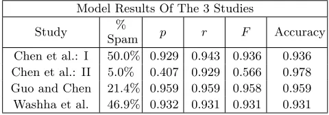
The model results from each of the three studies are pre-sented in Table 4. Precision (p), recall (r), F-measure (F), and accuracy are presented as defined in Section 2.3. Be-tween the two test sets of Chen et al., there was a sharp drop inF when the proportion of spam in the test set dropped. Upon further analysis it was discovered that when the total spam tweets decreased, the number of false positives rose drastically, lowering the precision of the random forest [2].

Each model displayed high accuracies (≥0.931). Exclud-ing test set II by Chen et al., all values ofF are above 0.93, showing that the models have high precision and recall.

Direct comparisons between models should be taken with reservation; each study measures something different. Chen et al. looked at individual tweets, Guo and Chen studied non-personal users, and Washha et al. studied spammers. That being stated, each study performs similar in terms of accuracy andF, excluding test set II from Chen et al.

Table 4: Model results from the 3 analyses studied: Chen et al., Guo and Chen, and Washha et al..

Model Results Of The 3 Studies Study %

Spam p r F Accuracy Chen et al.: I 50.0% 0.929 0.943 0.936 0.936 Chen et al.: II 5.0% 0.407 0.929 0.566 0.978 Guo and Chen 21.4% 0.959 0.959 0.958 0.959 Washha et al. 46.9% 0.932 0.931 0.931 0.931

5.

CONCLUSIONS

This paper summarized three unique ways of classifying spam tweets, spammers, and non-personal users using dif-ferent features. All models displayed high accuracies and all but test set II of Chen et al. showed high F-measures, indi-cating a high classification ability of the different models.

Chen et al. performed a novel analysis when noting that typically only 5% of tweets are spam and adjusting for this by creating a separate test set. Future work could reapply this notion to the work of Guo and Chen as well as that of Washha et al. to see how this change affects their analysis.

All three models showed that random forests, in combi-nation with particular features, can be used as strong clas-sifiers of spam, spammers, and non-personal users. In ad-dition, applications of random forests may have unexpected results when applied to real data if a realistic proportion of spam/spammers is not accounted for in the test set.

Acknowledgments

I thank my adviser, Peter Dolan, and my senior seminar professor, Elena Machkasova, for their invaluable advice and comments throughout the research and writing process. Ad-ditionally, I thank my alumni reviewer, Jacob Opdahl, for his revisions and comments during the review process.

6.

REFERENCES

[1] L. Breiman. Random forests.Machine learning, 45(1):5–32, 2001.

[2] C. Chen, J. Zhang, X. Chen, Y. Xiang, and W. Zhou. 6 million spam tweets: A large ground truth for timely twitter spam detection. In2015 IEEE International Conference on Communications (ICC), pages 7065–7070. IEEE, 2015.

[3] D. Guo and C. Chen. Detecting non-personal and spam users on geo-tagged twitter network.Transactions in GIS, 18(3):370–384, 2014.

[4] M. Kubat.An Introduction to Machine Learning. Springer Publishing Company, Incorporated, 1st edition, 2015.

[5] C. E. Shannon. A mathematical theory of

communication.ACM SIGMOBILE Mobile Computing and Communications Review, 5(1):3–55, 2001.