Throwing Buffon’s Needle with Mathematica »

Throwing Buffon’s

Needle with

Mathematica

Enis Siniksaran

It has long been known that Buffon’s needle experiments can be used to estimate p. Three main factors influence these experiments: grid shape, grid density, and needle length. In statistical literature, several experi-ments depending on these factors have been designed to increase the efficiency of the estimators of p and to use all the information as fully as possible. We wrote the package BuffonNeedle to carry out the most com-mon forms of Buffon’s needle experiments. In this article we review statisti-cal aspects of the experiments, introduce the package BuffonNeedle, discuss the crossing probabilities and asymptotic variances of the estimators, and describe how to calculate them using Mathematica.

‡

Introduction

known, it involves dropping a needle of length l at random on a plane grid of parallel lines of width d>l units apart and determining the probability of the needle crossing one of the lines. The desired probability is directly related to the value of p, which can then be estimated by Monte Carlo experiments. This point is one of the major aspects of its appeal. When p is treated as an unknown param-eter, Buffon’s needle experiments can be seen as valuable tools in applying the concepts of statistical estimation theory, such as efficiency, completeness, and sufficiency. For instance, in order to obtain better estimators of p, Kendall and Moran [2] and Diaconis [3] examine several aspects of the problem with a long needle (l>d). Morton [4] and Solomon [5] provide the general extension of the problem. Perlman and Wishura [6] investigate a number of statistical estimation procedures for p for the single, double, and triple grids. In their study, they show that moving from single to double to triple grid, the asymptotic variances of the estimators get smaller and hence more efficient estimators can be obtained. Wood and Robertson [7] introduce the concept of grid density and provide an alternative idea. They show that Buffon’s original single grid is actually the most efficient if the needle length is held constant (at the distance between lines on the

of grid material per unit area). In [8], Wood and Robertson investigate the ways of maximizing the information in Buffon’s experiments.

We organize this article as follows. In the first three sections, we review Buffon’s experiments on single, double, and triple grids and their statistical issues. In the next section, we introduce the features of the package BuffonNeedle. The functions in the package implement Monte Carlo experiments for the three types of grids. The results of each experiment are given in a table and in a picture. When the number of the needles thrown on each grid is large, very nice pictures exhibit the interface between chance and necessity. In the last two sections, we describe how to calculate the crossing probabilities in single- and double-grid experiments and the asymptotic variances of the estimators for each grid using

Mathematica.

‡

Single-Grid Experiment

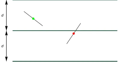
The single-grid form is Buffon’s well-known original experiment. A plane (table or floor) has parallel lines on it at equal distances d from each other. A needle of length l (l<d) is thrown at random on the plane. Figure 1 shows a single grid with two needles of length l representing two possible outcomes. The probabili-ties of crossing zero lines and one line are

(1)

p0=1-2 rq, p1=2 rq,

where r=lêd and q =1êp. These results can be found in many probability and statistics textbooks, for instance [5, 9, 10]. They are also explained in the “Calcu-lating the Crossing Probabilities in Single and Double Grids” section of this article.

d

d

Figure 1. Buffon’s needles on a single grid.

From equation (1), we can write

(2)

q = 1 p =

p1 2 r.

Let N1 be the number of times in n independent tosses that the needle crosses any line. Then the proportion of crossings p`<sub>1</sub>, a point estimator of p1, becomes p`₁=N1ên. Hence, we can write the point estimator of q in equation (2) as

(3)

q` = p ` 1

2 r =

N1 2r n.

The random variable N1 is binomially distributed with the parameters n and p1. q` is the uniformly minimum variance unbiased estimator (UMVUE). Further-more, it is the maximum likelihood estimator (MLE) of q and hence has 100% asymptotic efficiency in this experiment [6]. The variance of q` is then

(4) VarHq`L=Var N1

2 r n =

p1H1-p1L 4 r2 _n =

q_H1-2r qL

2n r =

q

2 n

1

r -2 q ,

which is minimized by taking r as close as possible to 1. Choosing needle length

l=d (r=1) ensures this purpose. In this case, the variance of q` becomes

(5) VarHq`L= q

2

2 n

1

q -2 .

In Buffon’s experiments, the parameter of main interest is p rather than q. The estimator of this parameter, p` =1êq`, is called Buffon’s estimator and can be obtained from equation (3) as

(6)

p` = 2 r p ` 1

.

It can also be expressed in terms of p`₀=N0ên

(7)

p` = 2 r

1-p`₀

,

where N0 is the number of times in n tosses that the needle does not cross any line. Using equation (6) or (7) and Monte Carlo methods, we can obtain empir-ical estimates of p for various values of r. The best estimate is expected at r=1 (l=d). Standard theory [11] ensures that Buffon’s estimator is an asymptotically unbiased, 100% efficient estimator of 1êq. Applying the delta method shows that its asymptotic variance is

(8) AVarHp`L= p

2

2 nK

p

which is, as expected, minimized at r=1. For this value of r, the asymptotic vari-ance of p` is

(9) AVarHp`L= p

2

2 nHp -2L. If it is evaluated at p =3.1416, we have

(10) AVarHp`L= 5.63

n .

‡

Double-Grid Experiment

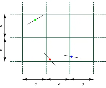
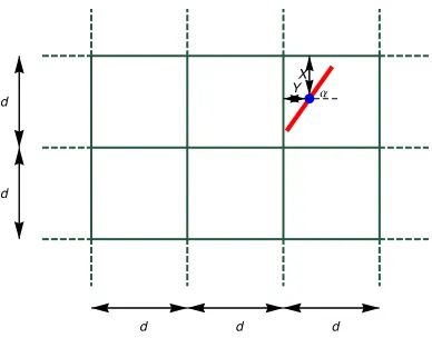
In the double-grid experiment, also called the Laplace extension of Buffon’s problem, a plane is covered with two sets of parallel lines where one set is orthog-onal to the other.

d

d

d d d

Figure 2. Buffon’s needles on a double grid.

In Figure 2, we see a double-grid plane and three needles of length l crossing zero, one, and two lines. These crossing probabilities are

(11)

p0=1-r H4-rL q, p1=2 r H2-rL q, p2=r2 q.

Let Ni be the number of times in n tosses that the needle crosses exactly i lines (i=0, 1, 2). Perlman and Wichura [6] showed that the random variable N1+N2 is distributed binomially with the parameters n and mq and is completely suffi-cient for q where m is 4r-r2_{. They also showed that the random variable}

is the UMVUE and has 100% asymptotic efficiency with the variance

(13) VarHq`L= q

n l m- q .

As in the case of a single grid, the variance of q` is minimized by r=1, or equiv-alently by l=d. Replacing N1+N2 with n-N0 in the right-hand side of equa-tion (12), we have

(14)

q` = n-N0 m n =

1

m 1 -N0

n =

1-p`₀

4 r-r2.

Then Buffon’s estimator, p` =1êq`, can be expressed as

(15)

p` = 4 r-r 2

1-p`₀

,

which can be used to obtain empirical estimates of p. By the delta method, we can obtain the asymptotic variance of p` as

(16) AVarHp`L= p

2I_{4 r-r}2_{- p}M n r Hr-4L , which is minimized at r=1. For this value of r, it becomes

(17) AVarHp`L= p

2

3nHp -3L.

When evaluated at p =3.1416, it is

(18) AVarHp`L= 0.466

n .

Compare the last equation with equation (10). Buffon’s estimator in the double-grid experiment is 5.63ê0.466>12 times as efficient as that in the single-grid experiment.

‡

Triple-Grid Experiment

d

d

2 d

3

Figure 3. Buffon’s needles on a triple grid.

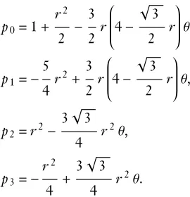
Figure 3 shows a triple-grid plane and four needles of length l crossing zero, one, two, and three lines. In [7], the crossing probabilities are given as

(19)

p0=1+ r2

2 -3

2 r 4 -3

2 r q,

p1= -5

4 r 2₊3

2 r 4 -3

2 r q,

p2=r2

-3 3

4 r 2 _q,

p3= -r2

4 +

3 3

4 r 2 _q.

Let Ni denote the number of times in n tosses that the needle crosses exactly i lines (i=0, 1, 2, 3). For this experiment, Perlman and Wichura [6] investigated the random variable N1+N2+N3 which is distributed binomially with the pa-rameters n and a q -1ê2 where a =3 rê2I4- 3 rê2M. They proposed, among others, the following unbiased estimator of q as a function of N1+N2+N3

(20)

q`= 1 a

N1+N2+N3

n +

1

By replacing N1+N2+N3 with n-N0, as in the other experiments, we obtain the same estimator as a function of N0

(21)

q` = 1 a

n-N0

n +

1

2 =

1

a

3

2-p

` 0 .

The variance of q` is

(22) VarHq`L= H2 a q -3L H2a q -1L

4a2 _n .

As in the cases of the single- and double-grid experiments, the variance of q` is minimized by taking r=1 (l=d).

From equation (21), Buffon’s estimator can be written as

(23)

p` = 2 a

3-2 p`₀

= 3 r I8- 3 rM

2I3-2p`₀M

.

For this experiment, the asymptotic variance of Buffon’s estimator is

(24) AVarHp`L= -K2 p2K-3 3 + pO K-3 3 +4pO

K-24+3 3 r+5prO K3rK-8+ 3 rO+2pI2+r2MOO ì K9n rK54K64-16 3 r+3r2_{O+ p}2_{K512-128 3 r}

-270r2_{+96 3 r}3_+27r4_{O+6pK-320 3 +}

168r+234 3 r2-306r3+27 3 r4OOO.

For r=1 and p =3.1416, it is

(25) AVarHp`L= 0.015781

n .

Comparing this with equations (10) and (18), we can infer that Buffon’s estimator in the triple-grid experiment is 0.466ê0.015781>29 times as efficient as in the double-grid experiment and 5.63ê0.015781>356 times as efficient as in the single-grid experiment (see Table 1). Now, we can conclude that when we increase the complexity of the grid, we can obtain tighter estimators of p. Wood and Robertson [7] investigated this conclusion. They introduced the notion of grid density, which is the average length of grid in a unit area and showed that when the experiments are standardized, Buffon’s estimator in a single grid is the most efficient. In their approach, when d=1, the single grid has unit grid den-sity, the double grid has grid density of two, and the triple grid has grid density of three. Hence, the standardization of experiments corresponds to r=1 in the single grid, r=1ê2 in the double grid and, finally, r=1ê3 in the triple grid. Replacing these values of r in equations (8), (16), and (24) and evaluating them at

Grid Type SingleHr=1L DoubleHr=1L TripleHr=1L AVarHp`L 5.63ên 0.466ên 0.015781ên

Table 1. Asymptotic variances of Buffon’s estimator for three grids.

Grid Type SingleHr=1L DoubleHr=1ê2L TripleHr=1ê3L

AVarHp`L 5.63ên 7.85ên 5.91ên

Table 2. Asymptotic variances of Buffon’s estimator for three standardized grids.

‡

The Package

The BuffonNeedle package is designed to throw needles on single, double, and triple grids. Copy the file BuffonNeedle.m (see Additional Material) into the

Mathematica@ AddOns @ Applications folder. The following command loads the program.

In[18]:= <<BuffonNeedle.m

There are three functions in this package: SingleGrid[n,r], DoubleGrid[n,r], and TripleGrid[n,r]. Here, n is the number of needles and r is the ratio of needle length to grid height (i.e., r=lêd), where n can be any integer, while r

is a real number on the interval H0, 1D.

SingleGrid[n,r] implements a single-grid Buffon’s experiment. It gives a table showing the number and frequency ratios of the two possible outcomes, together with the theoretical probabilities and the estimate of p defined in equation (7). The function also gives a picture of the simulation results. In the picture, the midpoints of the needles crossing any line are colored red, while those of needles crossing no line are colored green. The functions DoubleGrid[n,r] and TripleÖ

Grid[n,r] carry out similar processes for double and triple grids, respectively. In the picture of a double-grid experiment, the midpoints of the needles are colored green, blue, and red to show the three possible outcomes of zero, one, and two crossings. The estimate of p in this experiment is defined in equation (15). As in the other two cases, in a triple-grid experiment carried out by the function

TripleGrid[n,r], the four possible outcomes of zero, one, two, and three cross-ings are represented by four different colors of the midpoints of the needles. The estimate of p given in the table is defined in equation (23).

In[19]:= SingleGrid@10, .87D

***Results of throwing 10 needles of length l=0.87.d on a single grid***

Zero Crossing

One Crossing Number of Crossings 4 6 Frequency Ratio 0.4000 0.6000 Theoretical Probability 0.4461 0.5539

Estimate of Pi:2.9

Out[19]=

In[20]:= DoubleGrid@15, .76D

***Results of throwing 15 needles of length l=0.76.d on a double grid***

Zero Crossing

One Crossing

Two Crossings

Number of Crossings 2 11 2

Frequency Ratio 0.1333 0.7333 0.1333 Theoretical Probability 0.2162 0.6000 0.1839

Estimate of Pi:2.84123

In[21]:= TripleGrid@12, .70D

***Results of throwing 12 needles of length l=0.7.d on a triple grid***

Zero Crossing

One Crossing

Two Crossings

Three Crossings

Number of Crossings 2 8 2 0

Frequency Ratio 0.1667 0.6667 0.1667 0 Theoretical Probability 0.1107 0.5218 0.2874 0.08011

Estimate of Pi:2.6726

Out[21]=

In[22]:= SingleGrid@10 000, .91D

***Results of throwing 10000 needles of length l=0.91.d on a single grid***

Zero Crossing

One Crossing Number of Crossings 4145 5855 Frequency Ratio 0.4145 0.5855 Theoretical Probability 0.4207 0.5793

Estimate of Pi:3.10845

In[23]:= DoubleGrid@38 000, .85D

***Results of throwing 38000 needles of length l=0.85.d on a double grid***

Zero Crossing

One Crossing

Two Crossings Number of Crossings 5675 23 577 8748 Frequency Ratio 0.1493 0.6204 0.2302 Theoretical Probability 0.1477 0.6223 0.2300

Estimate of Pi:3.14756

Out[23]=

In[24]:= TripleGrid@28 000, 1D

***Results of throwing 28000 needles of length l=1.d on a triple grid***

Zero Crossing

One Crossing

Two Crossings

Three Crossings Number of Crossings 97 7000 16 392 4508 Frequency Ratio 0.003464 0.2500 0.5854 0.1610 Theoretical Probability 0.003637 0.2464 0.5865 0.1635

Estimate of Pi:3.14123

‡

Calculating the Crossing Probabilities in Single and

Double Grids

In this section, we show how to calculate the crossing probabilities in single- and double-grid experiments using Mathematica.

· Single-Grid Probabilities

In the single-grid experiment, two independent random variables with uniform distribution are defined to determine the relative position of the needle to the lines: the distance X of the needle’s midpoint to the closest line and the acute angle a formed by the needle (or its extension) and the line (Figure 4). It is seen that X can take any value between 0 and dê2 and a can take any value between 0 and pê2. The density functions of X and a are then given by

In[25]:= gdist1=UniformDistributionB:0,

d

2>F; fX=PDF@gdist1, xD

Out[26]= µ 2_d 0§x§ d₂

In[27]:= gdist2=UniformDistributionB:0,

Pi

2 >F; fa=PDF@gdist2,aD

Out[28]= µ 2_p 0§ a § p 2

Since X and a are independent, the joint density function is the product of the density function of X alone and the density function of a alone:

In[29]:= fX,a=

2

d 2

p

Out[29]= 4

dp

for 0§x§dê2, 0§ a § pê2.

From Figure 4, it is clear that the needle crosses the line when X§lê2 sina. The probability of this event is then

In[30]:= p1=‡ 0

pê2 ‡

0

Hlê2L*Sin@aD

fX,a„x „a

Out[30]= 2 l

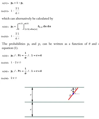
As there are two possible outcomes in the single-grid experiment, the probability that the needle does not cross any line is given by

In[31]:= p0=1-p1

Out[31]= 1 -2 l dp

which can alternatively be calculated by

In[32]:= p0=‡

0 pê2

‡

Hlê2L*Sin@aD

dê2

fX,a„x „a

Out[32]= 1 -2 l

dp

The probabilities p0 and p1 can be written as a function of q and r as in equation (1).

In[33]:= p0ê. PiØ

1

q ê. lØr*d

Out[33]= 1-2 rq

In[34]:= p1ê. PiØ

1

q ê. lØr*d

Out[34]= 2 rq

d d

X

lê2 lê2

a

Figure 4. The random variables in the single-grid experiment.

· Double-Grid Probabilities

In[38]:= gdist1=UniformDistributionB:0,

d 2>F; fX=PDF@gdist1, xD

Out[39]= µ 2_d 0§x§ d₂

In[40]:= fY=PDF@gdist1, yD

Out[40]= µ 2_d 0§y§ d₂

In[41]:= gdist2=UniformDistributionB:0,

Pi 2 >F; fa=PDF@gdist2,aD

Out[42]= µ 2_p 0§ a § p₂

As in the case of the single-grid experiment, the joint density function of X, Y, and a is the product of the density functions of X, Y, and a:

In[43]:= fX,Y,a= 2

d 2

d 2

p

Out[43]= 8

d2_p

for 0§x§dê2, 0§y§dê2, 0§ a § pê2.

In the double-grid experiment, there are four possible outcomes:

Ë The needle crosses a horizontal line while not crossing a vertical line.

Ë The needle crosses a vertical line while not crossing a horizontal line.

Ë The needle crosses both a vertical line and a horizontal line or, equiva-lently, the needle crosses two lines.

Ë The needle crosses neither a vertical line nor a horizontal line or, equivalently, the needle crosses no line.

The needle crosses a horizontal line but does not cross a vertical line when

X§lê2 sina and Y >lê2 cosa. The probability of this event is given by

In[44]:= p_{X Y}ê=‡

0 pê2

‡

Hlê2L*Cos@aD

dê2

‡ 0

Hlê2L*Sin@aD

fX,Y,a„x „y „a

Out[44]=

The needle crosses a vertical line but does not cross a horizontal line when

X>lê2 sina and Y § lê2 cosa. The probability of this event is given by

In[45]:= p_Xê _Y=‡

0 pê2

‡ 0

Hlê2L*Cos@aD

‡

Hlê2L*Sin@aD

dê2

fX,Y,a „x „y „a

Out[45]=

H2 d-lLl d2_p

Thus, the probability that the needle crosses exactly one line is

In[46]:= p1=p_{X Y}ê+p_Xê _Y

Out[46]=

2H2 d-lLl

d2_p

The needle crosses both the vertical line and the horizontal line when

X§lê2 sina and Y § lê2 cosa. The probability of this event is

In[47]:= p2=‡

0 pê2

‡ 0

Hlê2L*Cos@aD

‡ 0

Hlê2L*Sin@aD

fX,Y,a„x „y „a

Out[47]= l2

d2_p

Finally, the needle crosses neither the vertical line nor the horizontal line when

X>lê2 sina and Y >lê2 cosa. The probability of this event is

In[48]:= p0=‡

0 pê2

‡

Hlê2L*Cos@aD

dê2

‡

Hlê2L*Sin@aD

dê2

fX,Y,a„x „y „a

Out[48]= 1+

lH-4 d+lL

d2_p

The probabilities p0, p1, and p2 can be written as functions of q and r, as in equa-tion (11).

In[49]:= p0ê. PiØ

1

q ê. lØr*dêêSimplify

Out[49]= 1-4 rq +r2q

In[50]:= p1ê. PiØ

1

q ê. lØr*dêêSimplify

Out[50]= -2H-2+rLrq

In[51]:= p2ê. PiØ

1

q ê. lØr*dêêSimplify

d

d

d d d

X Y _a

Figure 5. The random variables in the double-grid experiment.

‡

Delta Method and Asymptotic Variance

Let a random variable Y be a function of the random variable X, that is,

Y =HHXL. When the function HHXL is nonlinear, it may not be possible to compute the true mean and the true variance of Y. One can, however, calculate estimates of the true mean and true variance. The delta method is a very useful way to find such estimates [12, 13] and is based on the Taylor expansion about the mean of X. Let the mean of X be m and the variance s2_{. Then the Taylor} expansion of the function HHXL about m to the third term is

(26)

H HXL=H HmL+H£HX- mL+1

2 H

″_{HX- mL}2_.

Taking the expectation of both sides, we obtain the approximate mean of Y = HHXL as

(27) AMean@H HXLD=E@H HXLD=H HmL+1

2 H

″_{HmL s}2_.

From the well-known identity of statistics

(28) Var@H HXLD=E 8H HXL-E@H HXLD<2,

the approximate variance, also called asymptotic variance, of Y =HHXL is

(29) AVar@H HXLD=@H£HmLD2 _s2_.

Thus, we can say that the random variable Y is distributed with the approximate mean HHmL+1ê2 H″HmL s2 _{and the approximate variance} @_H£_HmLD2 _s2

.

Buffon’s estimator is a nonlinear function of the random variable q`

vari-(p` =HHqL=1êq); hence, the delta method can be used to find its asymptotic vari-ance. From the previous sections, for each grid, we know EHq`L and VarHq`L. Then, in equation (29), substituting HHXL= p`, m = q, and s2_=VarHq`<sub>L from</sub> equations (5), (13), and (22), we can obtain the asymptotic variances of p` in equa-tions (8), (16), and (24) for each grid.

Alternatively, asymptotic variances of p` can be computed as follows [7, 11]

(30) AVar@p`D= @H

£_HqLD2

n I HqL . Here IHqL is the Fisher information number, given by

(31)

IHqL=‚

i

Ap_i″HqLE2 piHqL

,

where piHqL is the probability that the needle crosses i lines. These probabilities given in equations (1), (11), and (19) actually define a list for each grid as follows:

In[53]:= ProbSingle=81-2 rq, 2 rq<;

ProbDouble=91-rH4-rL q, 2rH2-rL q, r2 _q=;

ProbTriple=:1+r

2

2 -3

2 r 4 -3

2 r q,

-5

4 r 2₊3

2r 4 -3

2 r q, r

2_-3 3

4 r

2 _q,-r 2

4 +

3 3

4 r

2 _q>;

From equations (30) and (31), one can define the following functions to obtain the asymptotic variances:

In[56]:= deriv@expr_, var_D:=

HD@expr, varDL2 HexprL ; fisherInfo@list_, var_D:=

Total@Table@deriv@list@@iDD, varD,8i, Length@listD<DD;

aVar@list_, var_D:= HD@1êvar, varDL

2

Hn fisherInfo@list, varDL;

For each grid, therefore, the asymptotic variances are

In[59]:= aVar@ProbSingle,qD

Out[59]=

1

nq4_J2 r q +

4 r2

1-2 rqN

In[60]:= aVar@ProbDouble,qD

Out[60]=

1

nq4_J2H2-rLr

q +

r2

q +

H4-rL2_r2

In[61]:= aVar@ProbTriple,qD

Out[61]= 1ì nq4

27 r4

16Jr2_-3

4 3 r

2_qN

+ 27 r

4

16J-r₄2+ 3₄ 3 r2_qN +

9 r2_K4- 3 r

2 O

2

4K1+r2 2

-3 2 rK4

-3 r 2 OqO

+

9 r2_K4- 3 r

2 O

2

4K-5 r2

4 +

3 2 rK4

-3 r 2 OqO

Substituting q =1êp and factoring the expressions, we have

In[62]:= aVar@ProbSingle,qD ê.q Ø

1

p êêFactor

aVar@ProbDouble,qD ê.q Ø 1

p êêFactor

aVar@ProbTriple,qD ê.q Ø 1

p êêFactor

Out[62]=

p2_{Hp -2 rL} 2 n r

Out[63]=

-p2_{Hp -4 r+r}2_L

nH-4+rLr

Out[64]= -J2p2J-3 3 + pN J-3 3 +4pN

J-24+3 3 r+5prN J4p -24 r+3 3 r2_+2pr2_{NN í}

J9 n rJ3456-1920 3 p +512p2_{-864 3 r+1008pr} -128 3 p2_{r+162 r}2_{+1404 3 pr}2_-270p2_r2 -1836pr3_{+96 3 p}2_r3_{+162 3 pr}4_+27p2_r4_NN

which were previously given in equations (8), (16), and (24), respectively. For

r=1 and p =3.1416, we obtain the same values given in Table 1 for each grid.

In[65]:= aVar@ProbSingle,qD ê.q Ø

1

p ê. rØ1ê.p Ø3.1416

Out[65]=

5.6336

n

In[66]:= aVar@ProbDouble,qD ê.q Ø

1

p ê. rØ1ê.p Ø3.1416

Out[66]=

In[67]:= aVar@ProbTriple,qD ê.q Ø

1

p ê. rØ1ê.p Ø3.1416

Out[67]=

0.0157809

n

For the standardized experiments of Wood and Robertson [7], we can obtain the asymptotic variances given in Table 2 by substituting r=1, 1ê2, and 1ê3 for single, double, and triple grids, respectively.

In[68]:= aVar@ProbSingle,qD ê.q Ø

1

p ê. rØ1ê.p Ø3.1416

Out[68]=

5.6336 n

In[69]:= aVar@ProbDouble,qD ê.q Ø

1

p ê. rØ

1

2 ê.p Ø3.1416

Out[69]=

7.84835 n

In[70]:= aVar@ProbTriple,qD ê.q Ø

1

p ê. rØ

1

3 ê.p Ø3.1416

Out[70]=

5.90518

n

‡

Acknowledgments

I would like to thank the reviewers whose comments led to a substantial improve-ment in this article. I would also like to thank my colleague, M. H. Satman, for creating some of the functions in the package BuffonNeedle. Thanks to Dr. Aylin Aktukun for reading and commenting on numerous versions of this manuscript. This work is supported by the Scientific Research Projects Unit of Istanbul University.

‡

References

[1] G. L. Buffon, “Essai d’arithmétique morale,” Histoire naturelle, générale, et particulière, Supplément 4, 1777 pp. 685|713.

[2] M. G. Kendall and P. A. P. Moran, Geometrical Probability, New York: Hafner, 1963.

[3] P. Diaconis, “Buffon’s Problem with a Long Needle,” Journal of Applied Probability, 13, 1976 pp. 614|618.

[4] R. A. Morton, “The Expected Number and Angle of Intersections Between Random Curves in a Plane,” Journal of Applied Probability, 3, 1966 pp. 559|562.

[6] M. D. Perlman and M. J. Wichura, “Sharpening Buffon’s Needle,” American Statistician, 29(4), 1975 pp. 157|163.

[7] G. R. Wood and J. M. Robertson, “Buffon Got It Straight,” Statistics and Probability Letters, 37,1998 pp. 415|421.

[8] G. R. Wood and J. M. Robertson, “Information in Buffon Experiments,” Journal of Statistical Planning and Inferences, 66,1998 pp. 21|37.

[9] M. R. Spiegel, Probability and Statistics, Schaum’s Outline of Probability and Statistics, New York: McGraw-Hill, 1975 pp. 67|68.

[10] J. V. Uspensky, Introduction to Mathematical Probability, New York: McGraw-Hill, 1937, p. 252.

[11] C. R. Rao, Linear Statistical Inference and Its Applications, 2nd ed., New York: Wiley & Sons, 1973.

[12] G. W. Oehlert, “A Note on the Delta Method,” American Statistician, 46, 1992 pp. 27|29.

[13] J. A. Rice, Mathematical Statistics and Data Analysis, 2nd ed., Belmont, CA: Duxbury Press, 1994 p. 149.

‡

Additional Material

Available at www.mathematica-journal.com/data/uploads/2011/11/BuffonNeedle.m.

About the Author

Enis Siniksaran is an assistant professor at Istanbul University, Department of Economet-rics. His research interests include geometric approaches to statistical methods, robust statistical methods, and the methodology of econometrics. He has been working with

Mathematica since 1998. For details on his recent work dealing with the geometry of classical test statistics, in which all symbolic and numerical computations and graphical work are done using Mathematica, see library.wolfram.com/infocenter/Articles/5962.

Enis Siniksaran

Istanbul Universitesi, Iktisat Fak., Ekonometri Bolumu Beyaz“t, 34452, Istanbul, Turkey

[email protected]

E. Siniksaran, “Throwing Buffon's Needle with Mathematica,” The Mathematica Journal,

2011. dx.doi.org/doi:10.3888/tmj.11.1–4.