Evaluation of Financial Options Using Radial Basis Functions in Mathematica »

The Mathematica® Journal

Evaluation of Financial Options

Using Radial Basis Functions in

Mathematica

Michael Kelly

In the academic literature there are two common approaches for the evalu-ation of financial options. These are stochastic calculus and partial differ-ential equations. The former is the method of choice for statisticians and theoreticians, while the latter is the principal tool of physicists and com-puter scientists because it lends itself to practical implementation schemes. Occasionally small modifications such as linear regression and binomial trees are used, but these are usually treated within either of the two previ-ously mentioned fields. Rarely do the practitioners of these fields compare and contrast methodologies, let alone admit completely different ap-proaches. While Radial Basis Function (RBF) methodology has previously been applied to solving some differential equations, there are very few papers considering its applicability to financial mathematics. The purpose of this article is to show not only that RBF can solve many of the evalu-ation problems for financial options, but that with Mathematica it can do so with accuracy and speed.

‡

Introduction

A radial basis function (RBF) is a function fHx,xiL that depends only on the dis-tance r between xœd _{and a fixed point x}

i œd

(1) fHx,xiL= fH »»x-xi»»L.

Each function fHx,xiL is radially symmetric about the center xi. Since their dis-covery in the early 1970s by Hardy [1, 2], RBFs have become a primary tool for the interpolation of multidimensional scattered data. In the 1990s, Kansa [3, 4] showed that RBF methods are applicable to solving elliptic parabolic and some hyperbolic partial differential equations (PDEs). While this approach has some similarities with finite difference (FD) formulas, there are significant differences in that FD stencils typically extend over a subset of the data points at which derivative approximations are sought, and FD formulas are obtained by differenti-ating polynomial interpolants rather than RBF interpolants. But the fact that RBF methods allow the solution of parabolic PDEs means that they are applica-ble to the Black|Scholes PDE and hence to the evaluation of financial options.

The purpose of this article is to apply global RBFs within Mathematica as a spa-tial collocation scheme for solving European and American option pricing mod-els by extending and implementing the work in this area that has recently been done by Hon and Mao [5] and Fasshauer, Khaliq, and Voss [6]. While some re-sults have been presented, none of the papers mentioned actually exhibit any pro-grams or discuss the programming difficulties that are inherent in RBF models of parabolic PDEs. A number of Runge|Kutta time integration schemes are adopted for the time derivatives of the option model. We show that these schemes result in highly accurate approximations when compared with existing numerical techniques and are inherently more stable than the more commonly used finite element methods.

The purpose of this article is to apply global RBFs within Mathematica as a spa-tial collocation scheme for solving European and American option pricing mod-els by extending and implementing the work in this area that has recently been done by Hon and Mao [5] and Fasshauer, Khaliq, and Voss [6]. While some re-sults have been presented, none of the papers mentioned actually exhibit any pro-grams or discuss the programming difficulties that are inherent in RBF models of parabolic PDEs. A number of Runge|Kutta time integration schemes are adopted for the time derivatives of the option model. We show that these schemes result in highly accurate approximations when compared with existing numerical techniques and are inherently more stable than the more commonly used finite element methods.

‡

Radial Basis Function Methodology for the Black

|

Scholes

Partial Differential Equation

It has been shown by Black and Scholes [7] that, assuming the underlying asset price is risk-neutral, all European options satisfy a lognormal parabolic PDE, now called the Black|Scholes PDE. If we let VHS,tL be the value of the option with underlying asset S and elapsed time t, risk-free interest rate r, dividend yield q, and volatility or annualized standard deviation of the asset price s, then the equation governing all European options is:

(2) VH0,1L_{HS,tL+Hr-qLS V}H1,0L_HS,tL+1

2S

2_s2_VH2,0L_{HS,tL-r VHS,tL=0.}

Like all other PDEs, the specification of the boundary conditions determines the type of option studied. The initial condition for the backward PDE has the following maturity payoff function, with K being the strike and T the time of maturity:

(3) VHS,TL= maxHK-S, 0L for put,

maxHS-K, 0L for call.

It is shown in [7] for European options that with HzL as the cumulative distribu-tion funcdistribu-tion of the standard normal distribudistribu-tion, the explicit soludistribu-tion is given by

(4) VHS,tL = S e

-qIT-tM_Hd

1L-K e-rIT-tMHd2L for calls,

K e-rIT-tMH-d2L-S e-qIT-tMH-d1L for puts.

d1 =

logHSêKL+Ir-q+ s2_{ê2M HT-tL}

s T-t

d2 = d1- s T-t.

By taking the mathematical derivatives VH0,1L_{HS,tL of the European options in}

equation (4), we readily obtain the hedging greek deltas

(5) DHS,tL=VH1,0L_HS,tL= e-qIT-tMHd1L for calls,

-e-qIT-tM_H-d

1L for puts.

Let us make a transformation into the log space so that S=ey_{, where} VHey_{,tL=UHy,tL. Then observing that V}H1,0L_HS,tL=UH1,0L_Hy,tL∂

SHyL=

1

S U

H1,0L_{Hy,tL and furthermore that V}H2,0L_HS,tL= 1

S2 IU

H2,0L_Hy,tL-UH1,0L_Hy,tLM,

equations (2) and (3) now become

Let us make a transformation into the log space so that S=ey_{, where} VHey_{,tL=UHy,tL. Then observing that V}H1,0L_HS,tL=UH1,0L_Hy,tL∂

SHyL=

1

S U

H1,0L_{Hy,tL and furthermore that V}H2,0L_HS,tL= 1 S2 IU

H2,0L_Hy,tL-UH1,0L_Hy,tLM,

equations (2) and (3) now become

(6) UH0,1L_{Hy,tL+ r-q-}s

2

2 U

H1,0L_Hy,tL+1

2s

2_UH2,0L_{Hy,tL-r UHy,tL=0}

with initial condition

(7) UHy,TL= maxHK-e

y_{, 0L for put,} maxHey-K, 0L for call.

The RBF methodology is to represent the option function UHy,tL as a linear combination of RBFs f_iHyL,i=1, … ,N at the collocation points yi

(8) UHy,tL=‚

j=1

N

ajHtLfjHyL.

There are a number of different choices for the RBFs; the most common include

Hardy’s multiquadratic (MQ) fIy, yjM= k2+Iy-yjM and the Gaussian fIy, yjM= ‰-k

2_Iy-y

jM_{, where k is the shape parameter. Extensive research in [3, 4]}

and Goldberg et al. [8] has demonstrated that the MQ interpolation is superior when solving inhomogeneous PDEs, as is the case with the Black|Scholes equa-tion. The specification of k is the basis of ongoing research, but here we adopt the recommendation in [1] that k =minH »»x-xi»»L for collocation points xi. Sub-stituting equation (8) into (6) we now have a system of N linear equations, i=1, … ,N:

(9) UH0,1L_Hy

i,tL+ r-q -s2

2 U

H1,0L_Hy i,tL+

1

2s

2_UH2,0L_Hy

i,tL-r UHyi,tL=0,

which can be further reduced by observing that

(10) UH0,1LHyi,tL = ‚

j=1

N

a£_{jHtLfIyi, y}

jM

UH1,0LHyi,tL = ‚

j=1

N

ajHtLfH1,0LIyi, yjM

UH2,0LHyi,tL = ‚

j=1

N

ajHtLfH2,0LIyi, yjM,

where the partial derivatives of the MQ RBFs, initially described in equation (1) and in the preceding paragraph with the shape parameter k, can be easily deter-mined in Mathematica.

Evaluation of Financial Options Using Radial Basis Functions in Mathematica 335

In[103]:= y1_, y2_: y1y2

2_{ 2}

;

Dyi, yj, yi, Dyi, yj,yi, 2

Out[104]= 

yiyj

2_y iyj2

, 1

2_y iyj2

 yiyj 2

2_y

iyj2 32

Now define the following elements of the NäN matrices F, Fy, and Fy,y with the N-vector _aèHtL

(11) Fi,j= fIyi, yjM,IFyM_i,j= fH1,0LIyi, yjM,IFy,yM_i,j= fH2,0LIyi, yjM,aj=HaèL_j.

Substituting equations (10), (11), and the previous differentiation output into equation (9), while observing that the elements of equation (10) actually define matrix products, results in the following matrix equation:

(12) F aè£+1

2s

2_F

y,yaè + r-q -1

2s

2 _F

yaè -rF aè =0.

Solving equation (12) for _aè allows the estimation of UHy,tL_{= F ÿ aè}HtL and hence of the original option price VHS,tL. It has been shown by Powell [9] that the ma-trix F is invertible. This allows us to rewrite equation (12) as a mama-trix differential equation for _aè

(13) aè£= F-1_ÿ 1

2s

2_F

y,yaè + r-q -1

2s

2 _F

yaè -rF aè =B ÿ aè.

B is the following NäN matrix and since all of its components, such as F and the identity matrix I, are known it is readily computed:

(14) B=r I- r-q-1

2s

2 _F-1_{ÿ F}

y -1

2s

2_F-1_{ÿ F}

y,y.

There are two approaches to solving equation (13): analytical and a backward time integration scheme. Using the work in [9], it follows that, if F is invertible and the eigenvectors of B are independent, then equation (12) has a solution for aè in terms of its eigenvectors w_èi and eigenvalues li. Using Mathematica’s DSolve operator we can explicitly analyze possible solutions to equation (13).

In[105]:= Blockvec, matB, n2,

vec Arrayt&, n; matBArrayB1,2&,n, n;

DSolveThreadDvec, tmatB.vec, vec,t

Out[105]=

A very large output was generated. Here is a sample of it:

1t 



1 2t1_

1

2t1 _{C2 1} 1,2

1_1,12 _{41}

1,212,1112,2 2

C11

2 1 ,

2t 1

Show Less Show More Show Full Output Set Size Limit...

Choosing larger values for n, the dimension of the matrix B suggests the follow-ing general solution:

(15) aèHtL=‚

i=1

N

kielitw_èi.

Then taking the time derivative of both sides and recalling that l_iw_èi=B ÿw_èi

be-cause of the definition of 9li,w_èi= as the eigensystem of B, we get:

(16) a_è£HtL=‚

i=1

N

kielitliw_èi=‚ i=1

N

kielitB ÿw_èi=B÷‚ i=1

N

kielitw_èi=B ÿ aèHtL.

This result satisfies equation (13) and shows that (15) yields an analytical solution for _aèHtL. Further, define the vectors k_è, _lè, and U_èJy_è,tN that consist of the compo-nents ki, li, and UHyi,tL as well as the matrix W that has as columns the eigenvec-tors w_èi, i=1, … , N. Now observe that collocating equation (8) about the cen-tral points yj converts it into the explicit matrix equation

(17) U_èJy_è,tN_{= F ÿ aè}HtL= F ÿ‚

i=1

N

w_èikielit = F ÿ _W ÿ_k

è ÿelèt.

It can be seen from equation (17) that U_èJy_è,tN, and hence VHS,tL, can be calcu-lated once k_è is determined. Since the result holds for all values of time t, then it also holds for the initial condition expressed by equation (7) at maturity time T. Putting t=T in the above result yields

(18) k_{è =}W-1 _{ÿ F}-1 _ÿ

U_èJy_è,TN

elèT .

While this result is sufficient for an explicit solution that will cover European op-tions, it is not capable of calculating path-dependent options that have to be up-dated in a time-dependent manner. In fact, if we choose to again use the DSolve

operator for larger values of the dimension of the matrix B, then we will get very complicated polynomial expressions that have to be solved by the RootSum func-tion. Here is an example.

Evaluation of Financial Options Using Radial Basis Functions in Mathematica 337

While this result is sufficient for an explicit solution that will cover European op-tions, it is not capable of calculating path-dependent options that have to be up-dated in a time-dependent manner. In fact, if we choose to again use the DSolve

operator for larger values of the dimension of the matrix B, then we will get very complicated polynomial expressions that have to be solved by the RootSum func-tion. Here is an example.

In[106]:= Blockvec, matB, n3,

vec Arrayt&, n; matBArrayB1,2&,n, n;

DSolveThreadDvec, tmatB.vec, vec,t

Out[106]=

A very large output was generated. Here is a sample of it:

1t

C3RootSum22  1121 113,311,1 31.3273,119,20,119,1_2,2

31.3273,19.4459,118,0.1308,

119,13,3&, 1_11

1 &

1 C1RootSum1,1,1

Show Less Show More Show Full Output Set Size Limit...

For the purpose of calculating American-style options, we will consider times tn=T-nDt and define U_èJy_è,tnN=U_èn, aèHtnL= aèn. Now we use backward-differ-ence time integration schemes that can be any of the explicit first-order (BD1):

(19) aèn_{= aè}n-1_{- Dt B ÿ aè}n-1 _=II

N- Dt BM aèn-1,

the explicit second-order backward-difference time integration scheme (BD2):

(20) R1 = -DtB ÿ aèn-1

R2 = -DtB ÿ aèn-1+

R1

2

aèn

= aèn-1₊R1+R2

2 ,

the explicit fourth-order backward-difference time integration scheme (BD4):

(21) R1 = -DtB ÿ aèn-1

R2 = -DtB ÿ aèn-1+

R1

2

R3 = -DtB ÿ aèn-1+

R2

2 R4 = -DtB ÿIaèn-1+R3M

aèn

= aèn-1₊R1+2R2+2R3+R4

6 ,

or the implicit backward-difference time integration scheme (IDq):

(22) aèn

= aèn-1_{- Dt B ÿI}

q aèn-1 _{+H1- qL}

aèn_M.

‡

European Options Numerical Specification

· Analytical Results

In order to evaluate European options, we need to specify their boundary condi-tions. Remember that all options will satisfy the Black|Scholes PDE of equa-tion (2) with the initial condition of equation (3), but that for further differentia-tion between opdifferentia-tions we also need to specify the boundary condidifferentia-tions as SØ0 and SØ ¶:

(23) VH0,tL = K e

-rIT-tM _{for put,}

0 for call,

VHS,tL Ø 0 asSØ ¶ for put, SasSØ ¶ for call.

By using these equations we can now implement the numerical solution of Euro-pean options. Even though we have given equations for both call- and put-style options, for the sake of brevity and to avoid what would essentially be very simi-lar programs, we restrict ourselves to put options only. The time domain is subdi-vided into M subintervals, Dt= T

M, so that for any prior time tn=T-nDt, n lies in the range 0§n§M, with n=0 corresponding to the maturity date T. The spatial discretization will be for N collocation points yi, 1§i§N. The Mathe-matica program for the Black|Scholes European options and their deltas accord-ing to equations (4) and (5) can be readily implemented.

In[107]:= ClearAllNormPDF, NormCDF, d1, d2, BSCall, BSPut,

putDelta, callDelta,y, y, t,t,,,y,yy,inv, B,

, w, W, UT, kvec,, U, Vanalytical, DeltaAnalytical;

d1_, r_, q_, x_, y_, t_:Logxyrq 2_{2t  t ;}

d2_, r_, q_, x_, y_, t_:Logxyrq 2_{2t  t ;}

Evaluation of Financial Options Using Radial Basis Functions in Mathematica 339

In[107]:=

d2_, r_, q_, x_, y_, t_:Logxyrq 2_{2t  t ;}

NormCDFz_:1Erfz 2 2; NormPDFz_:Expz2_{2 2;}

BSCall_, r_, q_, S_, K_, T_: Sq T_{NormCDFd1, r, q, S, K, T}

Kr T_{NormCDFd2, r, q, S, K, T;}

BSPut_, r_, q_, S_, K_, T_:Kr T_{NormCDFd2, r, q, S, K, T}

Sq T_{NormCDFd1, r, q, S, K, T;}

putDelta_, r_, q_, S_, K_, T_:

q T_{NormCDFd1, r, q, S, K, T;}

callDelta_, r_, q_, S_, K_, T_:

q T_{NormCDFd1, r, q, S, K, T;}

putGamma_, r_, q_, S_, K_, T_DputDelta, r, q, S, K, T, S; callGamma_, r_, q_, S_, K_, T_DcallDelta, r, q, S, K, T, S; For the sake of reproducing actual prices, we specify the following market param-eters. The risk-free interest rate is 1%, the dividend yield is 0, the volatility is 30%, the strike is $100, S_min of 1 gives a y_min of 0, and logHSmaxL= ymax=6. Let

there be N =121 collocation points (Npts) and subdivide the time to maturity T =1 year into M =100 subintervals. We chose rather large values for M and N that can be reused later for the American options, but are more than sufficient for evaluating European options. We later consider the implicit time recursion model with q =0.5, which corresponds to the Crank|Nicolson FD scheme. An upper limit on recursion is set at 1000. Further, observe that we calculate not just one value for the analytical and approximation results but all of the possible val-ues for the option over its spatial and time domains.

In[118]:= Option parameters

r0.1; 0.3; q0; K100; T1; M100; 0.5; Smax 6_N;

Npts121; Smin1; $RecursionLimit  1000;0tT, tTntis time elapsed, 0nM, 1i,jNpts,

is time remaining, S y_{, yLogS, ymin0,SmaxExpymax}

Our purpose is to compare the exact results for European options from the given Black|Scholes formulas with the analytical results of equation (17), explicit for-mulas of equations (19) to (21), and the implicit time integration scheme of equa-tion (22). Note that fIyi, yjM is the RBF as described earlier in equations (1), (10), and (11). With S_min and Smax the smallest and largest values of the stock

price, then the spatial increment in the y domain with N (or Npts) collocation

points is Dy= logISmaxM-logISminM

N-1 and choosing k =4Dy in fIyi, yjM, we can now

de-fine F, Fy, and Fy,y according to (11) as:

In[119]:= yLogSmaxLogSmin Npts1; tTM;

y1_, y2_: y1y2216y2_;

 Tabley1, y2,y1, LogSmin, LogSmax,y,

y2, LogSmin, LogSmax,y;

In[119]:=

y2, LogSmin, LogSmax,y;

yTableEvaluateDy1, y2, y1,

y1, LogSmin, LogSmax,y,y2, LogSmin, LogSmax,y;

yyTableEvaluateDy1, y2, y1, y1,

y1, LogSmin, LogSmax,y,y2, LogSmin, LogSmax,y; The definition of the matrix B is then determined from (14) and used to calculate the eigensystem of B as :l_i,w_èi>. The initial condition of (7) is used to determine UHy,TL (or UT), which is substituted into (18) to calculate k_è (or kvec), and this is further substituted into (15) to yield _aèHtL.

In[123]:= invInverse;

Br IdentityMatrixNpts 2inv.yy2rq 22inv.y;

, wEigensystemB; WTransposew;

UTTableMaxKExpy, 0,y, LogSmin, LogSmax,y; kvecInverseW.inv.UTExpT;

t_:ReW.kvec Expt;

Initial and boundary conditions of (7) and (23) are used to obtain UH0,tL and UHy,TL. The general formulas for UHy,tL, 0§t§T, 0§ y§logHSmaxL can now

be specified by (17). Finally, recalling that y=logHSL, t is the elapsed time, and t is the time remaining, we can get the analytical formula for VHS,tL and its hedg-ing delta in terms of UHlogHSL,tL by simply taking the derivatives of the RBFs fIy, yjM.

In[130]:= U0, t_:K ExprTt; Uy_, T:MaxKExpy, 0; Uy_, t_ ; y LogSmax:0; Uy_, t_ ; yLogSmax:

Tabley, yj,yj, LogSmin, LogSmax,y.t; VanalyticalS_,_:ULogS, T ;

VanalyticalS_:TableLogS, yj,

yj, LogSmin, LogSmax,y.ReW.kvec;

DeltaAnalyticalS_:TableEvaluateDy, yj, y .yLogS,

yj, LogSmin, LogSmax,y.ReW.kvecS; GammaAnalyticalS_:

TableEvaluateDy, yj,y, 2 .yLogS,

yj, LogSmin, LogSmax,y.ReW.kvecS2_; · Explicit and Implicit Results

The explicit and implicit backward-difference time integration schemes given by equations (19) to (22) can now be implemented using straightforward Do loops. We start at time t=T with UHy,TL set to UT as determined by (7) and step back-ward through time, considering earlier times tn=T-nDt, while defining

U_èJy_è,tnN=U_èn, aèHtnL= aèn. There is one further modification that needs to be un-dertaken in each step of the Do loop; namely, that the boundary condition (23) must be satisfied. Note that T-t=T-tn=nDt in the exponent. This modifica-tion occurs at S=S_min and hence when y= y1. This necessitates the rewriting

of UHy1,tL =U1HtL (or U[[1]]).

Evaluation of Financial Options Using Radial Basis Functions in Mathematica 341

The explicit and implicit backward-difference time integration schemes given by equations (19) to (22) can now be implemented using straightforward Do loops. We start at time t=T with UHy,TL set to UT as determined by (7) and step back-ward through time, considering earlier times tn=T-nDt, while defining

U_èJy_è,tnN=U_èn, _aèHtnL_{= aè}n_{. There is one further modification that needs to be} un-dertaken in each step of the Do loop; namely, that the boundary condition (23) must be satisfied. Note that T-t=T-tn=nDt in the exponent. This modifica-tion occurs at S=S_min and hence when y= y1. This necessitates the rewriting

of UHy1,tL =U1HtL (or U[[1]]).

In[138]:= ClearAllU0,0, n,1,2,4,i, U1, U2, U4, Ui, Un, V1explicit, V2explicit, V4explicit, Vimplicit, Delta1Explicit,

Delta2Explicit, Delta4Explicit, DeltaImplicit; U0UT; 0  inv.U0;

ModuleUn, 10  0;

Do1nIdentityMatrixNpts t B.1n1; Un .1n; Un1K Expr nt; 1n inv.Un,n, 1, M;

ModuleUn, R1, R2,20  0;

DoR1 t B.2n1; R2IdentityMatrixNpts t B2.R1;

2n 2n1R1R22; Un .2n;

Un1K Expr nt; 2n inv.Un,n, 1, M; ModuleUn, R1, R2, R3, R4,40  0;

DoR1 t B.4n1; R2IdentityMatrixNpts t B2.R1; R3R1 t B.R22; R4R1 t B.R3;

4n 4n1R12 R22 R3R46; Un .4n; Un1K Expr nt; 4n inv.Un,n, 1, M;

ModuleUn, B2IdentityMatrixNpts  t B, B1, B1B2 t B;

i0  0; DoinInverseB1.B2.in1; Un .in; Un1K Expr nt; in inv.Un,n, 1, M;

Now the initial and boundary conditions according to equations (7) and (23) are specified.

In[144]:= U1y_, 0:MaxKExpy, 0; U2y_, 0:MaxKExpy, 0; U4y_, 0:MaxKExpy, 0; Uiy_, 0:MaxKExpy, 0; U1y_, n_Integer ; y LogSmax:0;

U2y_, n_Integer ; y LogSmax:0; U4y_, n_Integer ; y LogSmax:0; Uiy_, n_Integer ; y LogSmax:0;

Again the general formulas for UHy,tL, 0§t§T; 0§ y§logHSmaxL can now be

specified according to the left-hand side of equation (17). We can also get the ex-plicit and imex-plicit approximation formulas for VHS,tL by using the updated val-ues for _aèHtnL= aèn. The hedging delta formulas are given in terms of UHlogHSL,tL

by simply taking the derivatives of the RBFs fIy, yjM.

In[148]:= U1y_, n_Integer ; yLogSmax:

Tabley, yj,yj, LogSmin, LogSmax,y.1n; U2y_, n_Integer ; yLogSmax:

Tabley, yj,yj, LogSmin, LogSmax,y.2n; U4y_, n_Integer ; yLogSmax:

Tabley, yj,yj, LogSmin, LogSmax,y.4n; Uiy_, n_Integer ; yLogSmax:

;

In[148]:=

Uiy_, n_Integer ; yLogSmax:

Tabley, yj,yj, LogSmin, LogSmax,y.in; V1explicitS_, n_Integer:U1LogS, n;

V2explicitS_, n_Integer:U2LogS, n; V4explicitS_, n_Integer:U4LogS, n; VimplicitS_, n_Integer:UiLogS, n; V1explicitS_:

TableLogS, yj,yj, LogSmin, LogSmax,y.1M; V2explicitS_:TableLogS, yj,

yj, LogSmin, LogSmax,y.2M; V4explicitS_:TableLogS, yj,

yj, LogSmin, LogSmax,y.4M; VimplicitS_:TableLogS, yj,

yj, LogSmin, LogSmax,y.iM;

Delta1ExplicitS_:TableEvaluateDy, yj, y .yLogS,

yj, LogSmin, LogSmax,y.1MS;

Delta2ExplicitS_:TableEvaluateDy, yj, y .yLogS,

yj, LogSmin, LogSmax,y.2MS;

Delta4ExplicitS_:TableEvaluateDy, yj, y .yLogS,

yj, LogSmin, LogSmax,y.4MS;

DeltaImplicitS_:TableEvaluateDy, yj, y .yLogS,

yj, LogSmin, LogSmax,y.iMS;

Gamma1ExplicitS_:TableEvaluateDy, yj,y, 2 .

yLogS,yj, LogSmin, LogSmax,y.1MS2_;

Gamma2ExplicitS_:TableEvaluateDy, yj,y, 2 .

yLogS,yj, LogSmin, LogSmax,y.2MS2_;

Gamma4ExplicitS_:TableEvaluateDy, yj,y, 2 .

yLogS,yj, LogSmin, LogSmax,y.4MS2_;

GammaImplicitS_:TableEvaluateDy, yj,y, 2 .

yLogS,yj, LogSmin, LogSmax,y.iMS2_;

In[168]:= TableForm

TablePaddedFormN1,7, 4& S, BSPut, r, q, S, K, T, VanalyticalS, V1explicitS,

V2explicitS, V4explicitS, VimplicitS,

S, 80, 200, 10, TableHeadings

None,"S", "Exact", "Analytic", "BD1", "BD2", "BD4", "ID", TableAlignmentsCenter

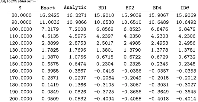
Evaluation of Financial Options Using Radial Basis Functions in Mathematica 343

Out[168]//TableForm=

S Exact Analytic BD1 BD2 BD4 ID

80.0000 16.2425 16.2271 15.9010 15.9039 15.9067 15.9069 90.0000 11.0036 10.9866 10.6530 10.6510 10.6489 10.6492 100.0000 7.2179 7.2008 6.8569 6.8523 6.8476 6.8479 110.0000 4.6135 4.5975 4.2397 4.2350 4.2303 4.2306 120.0000 2.8899 2.8753 2.5017 2.4985 2.4953 2.4956 130.0000 1.7825 1.7696 1.3801 1.3790 1.3778 1.3781 140.0000 1.0870 1.0756 0.6715 0.6722 0.6729 0.6732 150.0000 0.6575 0.6474 0.2304 0.2325 0.2345 0.2348 160.0000 0.3955 0.3867 0.0416 0.0386 0.0357 0.0353 170.0000 0.2371 0.2297 0.2084 0.2049 0.2015 0.2012 180.0000 0.1419 0.1366 0.3105 0.3067 0.3031 0.3027 190.0000 0.0849 0.0826 0.3725 0.3686 0.3649 0.3645 200.0000 0.0509 0.0532 0.4094 0.4055 0.4018 0.4014

Table 1. European put option prices determined by analytic, explicit, and implicit RBF methods.

In[169]:= TableFormTable

PaddedFormN1,7, 4& S, putDelta, r, q, S, K, T, DeltaAnalyticalS, Delta1ExplicitS,

Delta2ExplicitS, Delta4ExplicitS, DeltaImplicitS,

S, 80, 200, 10, TableHeadings

None,"S", "Exact", "Analytic", "BD1",

"BD2", "BD4", "ID ", TableAlignmentsCenter Out[169]//TableForm=

S Exact Analytic BD1 BD2 BD4 ID  80.0000 0.6028 0.6030 0.6037 0.6043 0.6048 0.6048 90.0000 0.4474 0.4475 0.4484 0.4488 0.4492 0.4491 100.0000 0.3144 0.3144 0.3156 0.3157 0.3158 0.3158 110.0000 0.2116 0.2114 0.2129 0.2128 0.2128 0.2128 120.0000 0.1376 0.1375 0.1391 0.1389 0.1387 0.1387 130.0000 0.0873 0.0871 0.0886 0.0884 0.0882 0.0882 140.0000 0.0543 0.0541 0.0555 0.0553 0.0552 0.0552 150.0000 0.0333 0.0331 0.0343 0.0342 0.0341 0.0341 160.0000 0.0202 0.0200 0.0211 0.0210 0.0210 0.0210 170.0000 0.0122 0.0120 0.0129 0.0129 0.0129 0.0129 180.0000 0.0073 0.0070 0.0079 0.0079 0.0079 0.0079 190.0000 0.0044 0.0040 0.0048 0.0048 0.0048 0.0047 200.0000 0.0026 0.0020 0.0028 0.0028 0.0028 0.0028

Table 2. European put option deltas determined by analytic, explicit, and implicit RBF methods.

In[170]:= TableFormTable

PaddedFormN1,7, 4& S, putGamma, r, q, S, K, T, GammaAnalyticalS, Gamma1ExplicitS,

Gamma2ExplicitS, Gamma4ExplicitS, GammaImplicitS,

S, 80, 200, 10, TableHeadings

None,"S", "Exact", "Analytic", "BD1",

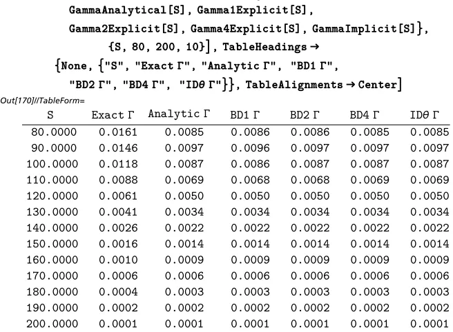
"BD2", "BD4", "ID ", TableAlignmentsCenter Out[170]//TableForm=

S Exact Analytic BD1 BD2 BD4 ID  80.0000 0.0161 0.0085 0.0086 0.0086 0.0085 0.0085 90.0000 0.0146 0.0097 0.0096 0.0097 0.0097 0.0097 100.0000 0.0118 0.0087 0.0086 0.0087 0.0087 0.0087 110.0000 0.0088 0.0069 0.0068 0.0068 0.0069 0.0069 120.0000 0.0061 0.0050 0.0050 0.0050 0.0050 0.0050 130.0000 0.0041 0.0034 0.0034 0.0034 0.0034 0.0034 140.0000 0.0026 0.0022 0.0022 0.0022 0.0022 0.0022 150.0000 0.0016 0.0014 0.0014 0.0014 0.0014 0.0014 160.0000 0.0010 0.0009 0.0009 0.0009 0.0009 0.0009 170.0000 0.0006 0.0006 0.0006 0.0006 0.0006 0.0006 180.0000 0.0004 0.0003 0.0003 0.0003 0.0003 0.0003 190.0000 0.0002 0.0002 0.0002 0.0002 0.0002 0.0002 200.0000 0.0001 0.0001 0.0001 0.0001 0.0001 0.0001

Table 3. American put option gammas determined by the Black|Scholes theory and by the analytic, explicit, and implicit RBF methods.

‡

American Options Numerical Specification

· Analytical Results

American options will satisfy the same boundary conditions of equation (23) as European options when SØ0 and SØ ¶, but must also satisfy the early exercise condition. This means that the current American value V_AHSt,tL is the maximum of the conditional expected future discounted value

Ie-rDt_VHSt

+Dt, t+ DtL _tM=VEHS,tL, which is the same as the European op-tion price and the exercise price K-St. That is,

(24) V_AHSt,tL=maxHV_EHSt,tL, K-StL=maxHV_EHSt,tL, UHlogHStL,TLL.

While we can implement this formula directly into the RBF formalism simply by taking the European option code in the previous section and comparing it with the exercise prices, this will not yield satisfactory results. The American options are path-dependent and can be exercised at any time, so they do not have one fi-nal boundary at maturity, but an infinite number of boundaries that describe the moving free boundary. There is no explicit formula for the American put, and it is likely that there will only ever be numerical approximations.

Evaluation of Financial Options Using Radial Basis Functions in Mathematica 345

In[171]:= ClearAllVAmerAnalytical, DeltaAmerAnalytical;

VAmerAnalyticalS_,_:MaxULogS, T , ULogS, T; VAmerAnalyticalS_:

MaxTableLogS, yj,yj, LogSmin, LogSmax,y.

ReW.kvec, KS, 0; DeltaAmerAnalyticalS_:Max

TableEvaluateDy, yj, y .yLogS,

yj, LogSmin, LogSmax,y.ReW.kvecS,1; GammaAmerAnalyticalS_:

TableEvaluateDy, yj,y, 2 .yLogS,

yj, LogSmin, LogSmax,y.ReW.kvecS2_; · Explicit and Implicit Results

The explicit and implicit backward-difference time integration schemes given by equations (19) to (22) can again be implemented using Do loops. As before, start at time t=T with UHy,TL set to UT as determined by (7) and step backward through time considering earlier times tn=T-nDt while defining

U_èJy_è,tnN=U_èn, aèHtnL= aèn. Again observe that T-t=T-tn=nDt in the expo-nent. As with the European options, there are further modifications that need to be undertaken in each step of the Do loop; namely, that the exercise condi-tion (23) must be satisfied for all points yi. At each time step tn and each colloca-tion point yi we determine the ith European option value of U_èn and then com-pare it with the exercise value K-Si_=K-eyi =K-S

mineHi-1LDy.

In[176]:= ClearAllUn,1a,2a,4a,ia, U1Amer, U2Amer, U4Amer, UiAmer, V1AmerExplicit, V2AmerExplicit, V4AmerExplicit, ViAmerImplicit, Delta1AmerExplicit,

Delta2AmerExplicit, Delta4AmerExplicit, DeltaAmerImplicit; U0UT; 0  inv.U0;

ModuleUn, 1a0  0;

Do1anIdentityMatrixNpts t B.1an1; Un .1an; DoUniMaxUni, KSmin Expi1y,i, 1, Npts;

1an inv.Un,n, 1, M; ModuleUn, R1, R2,2a0  0;

DoR1 t B.2an1; R2IdentityMatrixNpts t B2.R1;

2an 2an1R1R22; Un .2an;

DoUniMaxUni, KSmin Expi1y,i, 1, Npts;

2an inv.Un,n, 1, M;

ModuleUn, R1, R2, R3, R4,4a0  0;

DoR1 t B.4an1; R2IdentityMatrixNpts t B2.R1; R3R1 t B.R22; R4R1 t B.R3;

4an 4an1R12 R22 R3R46; Un .4an;

DoUniMaxUni, KSmin Expi1y,i, 1, Npts;

, ;

In[176]:=

DoUniMaxUni, KSmin Expi1y,i, 1, Npts;

4an inv.Un,n, 1, M;

ModuleUn, B2IdentityMatrixNpts  t B, B1, B1B2 t B;

ia0  0; DoianInverseB1.B2.ian1; Un .ian; DoUniMaxUni, KSmin Expi1y,i, 1, Npts;

ian inv.Un,n, 1, M;

Here the initial and boundary conditions according to equations (7) and (23) are specified.

In[182]:= U1Amery_, 0:MaxKExpy, 0; U2Amery_, 0:MaxKExpy, 0; U4Amery_, 0:MaxKExpy, 0; UiAmery_, 0:MaxKExpy, 0;

U1Amery_, n_Integer ; y LogSmax:0; U2Amery_, n_Integer ; y LogSmax:0; U4Amery_, n_Integer ; y LogSmax:0; UiAmery_, n_Integer ; y LogSmax:0;

Again, the general formulas for UHy,tL, 0§t§T, 0§ y§logHSmaxL can now be

specified according to the left-hand side of equation (17). We can also get the explicit and implicit approximation formulas for VHS,tL by using the updated val-ues for _aèHtnL= aèn. The hedging delta formulas are given in terms of UHlogHSL,tL

by simply taking the derivatives of the RBFs fIy, yjM.

In[186]:= U1Amery_, n_Integer ; yLogSmax:

Tabley, yj,yj, LogSmin, LogSmax,y.1an; U2Amery_, n_Integer ; yLogSmax:

Tabley, yj,yj, LogSmin, LogSmax,y.2an; U4Amery_, n_Integer ; yLogSmax:

Tabley, yj,yj, LogSmin, LogSmax,y.4an; UiAmery_, n_Integer ; yLogSmax:

Tabley, yj,yj, LogSmin, LogSmax,y.ian; V1AmerExplicitS_, n_Integer:

MaxU1AmerLogS, n, U1AmerLogS, 0; V2AmerExplicitS_, n_Integer:

MaxU2AmerLogS, n, U2AmerLogS, 0; V4AmerExplicitS_, n_Integer:

MaxU4AmerLogS, n, U4AmerLogS, 0; ViAmerImplicitS_, n_Integer:

MaxUiAmerLogS, n, UiAmerLogS, 0; V1AmerExplicitS_:MaxTableLogS, yj,

yj, LogSmin, LogSmax,y.1aM, KS, 0; V2AmerExplicitS_:MaxTableLogS, yj,

yj, LogSmin, LogSmax,y.2aM, KS, 0; V4AmerExplicitS_:MaxTableLogS, yj,

. , , 0;

Evaluation of Financial Options Using Radial Basis Functions in Mathematica 347

In[186]:=

V4AmerExplicitS_:MaxTableLogS, yj,

yj, LogSmin, LogSmax,y.4aM, KS, 0; ViAmerImplicitS_:MaxTableLogS, yj,

yj, LogSmin, LogSmax,y.iaM, KS, 0; Delta1AmerExplicitS_:TableEvaluateDy, yj, y .

yLogS,yj, LogSmin, LogSmax,y.1aMS; Delta2AmerExplicitS_:TableEvaluateDy, yj, y .

yLogS,yj, LogSmin, LogSmax,y.2aMS; Delta4AmerExplicitS_:TableEvaluateDy, yj, y .

yLogS,yj, LogSmin, LogSmax,y.4aMS; DeltaAmerImplicitS_:TableEvaluateDy, yj, y .

yLogS,yj, LogSmin, LogSmax,y.iaMS; Gamma1AmerExplicitS_:TableEvaluateDy, yj,y, 2 .

yLogS,yj, LogSmin, LogSmax,y.1aMS2_;

Gamma2AmerExplicitS_:TableEvaluateDy, yj,y, 2 .

yLogS,yj, LogSmin, LogSmax,y.2aMS2_;

Gamma4AmerExplicitS_:TableEvaluateDy, yj,y, 2 .

yLogS,yj, LogSmin, LogSmax,y.4aMS2_;

GammaAmerImplicitS_:TableEvaluateDy, yj,y, 2 .

yLogS,yj, LogSmin, LogSmax,y.iaMS2_;

For the sake of calculating actual prices, we use the same market parameters as before. As with the European options, observe that we calculate not just one value for the analytical and approximation results but all of the possible values for the American put option over its spatial and time domains. The time taken for these calculations is only incrementally longer than for the European case. In or-der to compare the RBF values for the American put with other schemes, we use the equal jumps additive binomial model described in Clewlow and Strickland [10], Chapter 2 and implemented here in Mathematica.

In[206]:= EqualJumpsAdditiveBinomialAmericanPut

S_ ? NumberQ, K_ ? NumberQ, r_ ? NumberQ, q_ ? NumberQ, sig_ ? NumberQ, T_ ? NumberQ, n_ ? NumberQ :

Modulei, j, dt  Tn, nu  rq0.5 sig ^ 2, dx, pu, pd, disc, eqdt, dpu, dpd, edx, St, C, dx Sqrtsig ^ 2 dtnu dt^ 2;

pu 12nu dtdx2; pd  1pu; disc  Expr dt; eqdt  Expq dt; dpu  disc pu; dpd  disc pd; edx Expdx;

Stn S Expn dx;

DoStj  Stj1edx,j,n1, n; DoCj  Max0, KStj,j,n, n, 2;

DoCj  dpu Cj1dpd Cj1; Stj  eqdt Stj; Cj MaxCj, KStj ,i, n1, 0,1,j,i, i, 2; C0 

We use this function with a large number N =500 steps to calculate highly accu-rate American put prices at the same stock values as for the European options. By varying the stock values by the incremental amount of DS=$0 .2, we can

We use this function with a large number N =500 steps to calculate highly accu-rate American put prices at the same stock values as for the European options. By varying the stock values by the incremental amount of DS =$0 .2, we can addi-tionally get values for the American put deltas.

In[207]:= binomialTree TableEqualJumpsAdditiveBinomialAmericanPut S, K, r, 0,, T, 500,S, 80, 200, 10

Out[207]= 20.2674, 13.1197, 8.33587, 5.21252, 3.20937, 1.95432, 1.18057, 0.706511, 0.423226, 0.251961, 0.149678, 0.0890653, 0.0531858

In[208]:= binomialTree2 

TableEqualJumpsAdditiveBinomialAmericanPutS, K, r, 0,, T, 500,

S, 80.2, 200.2, 10.0

Out[208]= 20.0961, 13.0046, 8.26003, 5.16277, 3.17714, 1.93422, 1.1686, 0.699655, 0.418883, 0.24923, 0.147999, 0.0880566, 0.0525953

In[209]:= binDelta  binomialTree2binomialTree0.2 Out[209]= 0.856572,0.575645,0.379222,0.248721,

0.161147,0.100498,0.0598567,0.034283,0.0217178,

0.0136589,0.00839964,0.00504329,0.00295229

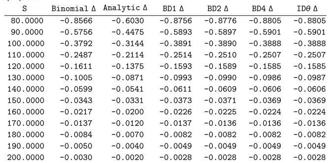
In Tables 4 and 5 we can see that while the RBF time integration schemes work very well to approximate the American put, the analytical result is not a suffi-ciently sensitive measure of the influence of the moving boundary.

In[210]:= TableFormTablePaddedFormN1,7, 4& 

S, binomialTreeS107, VAmerAnalyticalS, V1AmerExplicitS,

V2AmerExplicitS, V4AmerExplicitS, ViAmerImplicitS,

S, 80, 200, 10, TableHeadingsNone,

"S", "Binomial", "Analytic", "BD1", "BD2", "BD4", "ID", TableAlignmentsCenter

Out[210]//TableForm=

S Binomial Analytic BD1 BD2 BD4 ID

80.0000 20.2674 20.0000 20.1950 20.1914 20.1850 20.1848 90.0000 13.1197 10.9866 12.9464 12.9317 12.9172 12.9180 100.0000 8.3359 7.2008 8.1081 8.0926 8.0785 8.0797 110.0000 5.2125 4.5975 4.9468 4.9343 4.9234 4.9244 120.0000 3.2094 2.8753 2.9239 2.9155 2.9083 2.9092 130.0000 1.9543 1.7696 1.6526 1.6481 1.6445 1.6452 140.0000 1.1806 1.0756 0.8651 0.8638 0.8631 0.8637 150.0000 0.7065 0.6474 0.3824 0.3835 0.3847 0.3852 160.0000 0.4232 0.3867 0.0887 0.0913 0.0938 0.0943 170.0000 0.2520 0.2297 0.0000 0.0000 0.0000 0.0000 180.0000 0.1497 0.1366 0.0000 0.0000 0.0000 0.0000 190.0000 0.0891 0.0826 0.0000 0.0000 0.0000 0.0000 200.0000 0.0532 0.0532 0.0000 0.0000 0.0000 0.0000

Table 4. American put option prices determined by the binomial and analytic, explicit, and implicit RBF methods.

Evaluation of Financial Options Using Radial Basis Functions in Mathematica 349

In[211]:= TableForm

TablePaddedFormN1,7, 4& S, binDeltaS107, DeltaAmerAnalyticalS,

Delta1AmerExplicitS, Delta2AmerExplicitS, Delta4AmerExplicitS, DeltaAmerImplicitS,

S, 80, 200, 10, TableHeadings

None,"S", "Binomial", "Analytic", "BD1", "BD2", "BD4", "ID ", TableAlignmentsCenter Out[211]//TableForm=

S Binomial Analytic BD1 BD2 BD4 ID  80.0000 0.8566 0.6030 0.8756 0.8776 0.8805 0.8805 90.0000 0.5756 0.4475 0.5893 0.5897 0.5901 0.5901 100.0000 0.3792 0.3144 0.3891 0.3890 0.3888 0.3888 110.0000 0.2487 0.2114 0.2514 0.2510 0.2507 0.2507 120.0000 0.1611 0.1375 0.1593 0.1589 0.1585 0.1585 130.0000 0.1005 0.0871 0.0993 0.0990 0.0986 0.0987 140.0000 0.0599 0.0541 0.0611 0.0609 0.0606 0.0606 150.0000 0.0343 0.0331 0.0373 0.0371 0.0369 0.0369 160.0000 0.0217 0.0200 0.0226 0.0225 0.0224 0.0224 170.0000 0.0137 0.0120 0.0137 0.0136 0.0136 0.0136 180.0000 0.0084 0.0070 0.0082 0.0082 0.0082 0.0082 190.0000 0.0050 0.0040 0.0049 0.0049 0.0049 0.0049 200.0000 0.0030 0.0020 0.0028 0.0028 0.0028 0.0028

Table 5. American put option deltas determined by the binomial and analytic, explicit, and implicit RBF methods.

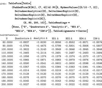
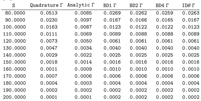
A final check on the accuracy of the results for American options can be obtained by loading the powerful financial software UnRisk (www.unriskderivatives.com). It uses compiled backward-recursive path integration over a large grid to obtain highly accurate estimates of path-dependent and American option values. The values returned by the calculation are {Put value, Delta, Gamma, Theta, Vega, VolConvexity, DeltaVega}. In Tables 6, 7, and 8 we can see that while the RBF backward-integration methodology works very well to approximate the American put, the analytical result is still not sufficiently sensitive to the behavior of the moving boundary.

In[212]:= Needs"UnRisk`UnRiskFrontEnd`"; MyEquities

TableMakeEquityS, EquityYieldq,S, 80, 200, 10; MyAmericanPutsTableMakeVanillaEquityOption

MyEquitiesi, K,2007, 4, 23, OptionType"Put", ExerciseType"American",i, 13;

MyYieldCurveMakeYieldCurver; MyVolCurve MakeVolatilityCurve; M100;

In[216]:= MyAmerValues

TableValuateMyAmericanPutsi,2006, 4, 23,2006, 4, 24, MyVolCurve, MyYieldCurve, CalculateVegaTrue,i, 13; TableFormMapPaddedFormN1,7, 4&,

JoinTransposeRange80, 200, 10, MyAmerValues, 2,

2, TableHeadings

None,"S", "Put", "Delta", "Gamma", "Theta", "Vega", "VolConvexity", "DeltaVega", TableAlignmentsCenter Out[216]//TableForm=

S Put Delta Gamma Theta Vega VolConvexity DeltaVega 80.0000 20.1072 0.8937 0.0513 0.0176 0.0973 0.0445 0.0426 90.0000 12.9840 0.5784 0.0230 0.0051 0.3113 0.0042 0.0098 100.0000 8.2379 0.3822 0.0163 0.0074 0.3579 0.0008 0.0003 110.0000 5.1387 0.2465 0.0111 0.0077 0.3342 0.0033 0.0044 120.0000 3.1598 0.1556 0.0073 0.0070 0.2797 0.0069 0.0061 130.0000 1.9209 0.0965 0.0047 0.0058 0.2185 0.0095 0.0060 140.0000 1.1578 0.0590 0.0029 0.0045 0.1625 0.0109 0.0051 150.0000 0.6937 0.0357 0.0018 0.0034 0.1167 0.0109 0.0040 160.0000 0.4140 0.0214 0.0011 0.0024 0.0816 0.0097 0.0030 170.0000 0.2465 0.0128 0.0007 0.0017 0.0558 0.0081 0.0022 180.0000 0.1467 0.0076 0.0004 0.0012 0.0376 0.0065 0.0015 190.0000 0.0873 0.0045 0.0002 0.0008 0.0251 0.0051 0.0010 200.0000 0.0520 0.0027 0.0001 0.0005 0.0166 0.0038 0.0007

In[217]:= TableFormTablePaddedFormN1,7, 4& 

S, MyAmerValuesS107, 1, VAmerAnalyticalS, V1AmerExplicitS,

V2AmerExplicitS, V4AmerExplicitS, ViAmerImplicitS,

S, 80, 200, 10, TableHeadingsNone,

"S", "Quadrature", "Analytic", "BD1", "BD2", "BD4", "ID", TableAlignmentsCenter

Out[217]//TableForm=

S Quadrature Analytic BD1 BD2 BD4 ID

80.0000 20.1072 20.0000 20.2411 20.2400 20.2364 20.2347 90.0000 12.9840 10.9926 13.1319 13.1182 13.1043 13.1045 100.0000 8.2379 7.2071 8.3540 8.3375 8.3225 8.3232 110.0000 5.1387 4.6041 5.2226 5.2080 5.1953 5.1961 120.0000 3.1598 2.8822 3.2173 3.2063 3.1970 3.1978 130.0000 1.9209 1.7766 1.9584 1.9512 1.9453 1.9459 140.0000 1.1578 1.0828 1.1811 1.1770 1.1740 1.1743 150.0000 0.6937 0.6548 0.7072 0.7054 0.7043 0.7045 160.0000 0.4140 0.3943 0.4216 0.4211 0.4212 0.4214 170.0000 0.2465 0.2376 0.2513 0.2517 0.2524 0.2525 180.0000 0.1467 0.1445 0.1509 0.1517 0.1528 0.1528 190.0000 0.0873 0.0907 0.0932 0.0942 0.0954 0.0954 200.0000 0.0520 0.0615 0.0619 0.0630 0.0642 0.0642

Table 6. American put option prices determined by the quadrature and analytic, explicit, and implicit RBF methods.

Evaluation of Financial Options Using Radial Basis Functions in Mathematica 351

In[218]:= TableFormTable

PaddedFormN1,7, 4& S, MyAmerValuesS107, 2, DeltaAmerAnalyticalS, Delta1AmerExplicitS,

Delta2AmerExplicitS, Delta4AmerExplicitS, DeltaAmerImplicitS,

S, 80, 200, 10, TableHeadings

None,"S", "Quadrature", "Analytic", "BD1", "BD2", "BD4", "ID ", TableAlignmentsCenter Out[218]//TableForm=

S Quadrature Analytic BD1 BD2 BD4 ID  80.0000 0.8937 0.6030 0.8556 0.8552 0.8571 0.8576 90.0000 0.5784 0.4475 0.5799 0.5801 0.5806 0.5807 100.0000 0.3822 0.3143 0.3849 0.3846 0.3845 0.3846 110.0000 0.2465 0.2114 0.2491 0.2487 0.2483 0.2484 120.0000 0.1556 0.1374 0.1579 0.1574 0.1570 0.1571 130.0000 0.0965 0.0871 0.0983 0.0979 0.0976 0.0976 140.0000 0.0590 0.0541 0.0602 0.0600 0.0598 0.0598 150.0000 0.0357 0.0331 0.0364 0.0363 0.0361 0.0361 160.0000 0.0214 0.0200 0.0219 0.0217 0.0216 0.0217 170.0000 0.0128 0.0120 0.0130 0.0129 0.0129 0.0129 180.0000 0.0076 0.0070 0.0076 0.0075 0.0075 0.0075 190.0000 0.0045 0.0040 0.0043 0.0042 0.0042 0.0042 200.0000 0.0027 0.0020 0.0022 0.0022 0.0022 0.0022

Table 7. American put option deltas determined by the quadrature and analytic, explicit, and implicit RBF methods.

In[219]:= TableFormTable

PaddedFormN1,7, 4& S, MyAmerValuesS107, 3, GammaAmerAnalyticalS, Gamma1AmerExplicitS,

Gamma2AmerExplicitS, Gamma4AmerExplicitS, GammaAmerImplicitS,

S, 80, 200, 10, TableHeadings

None,"S", "Quadrature", "Analytic", "BD1", "BD2", "BD4", "ID ", TableAlignmentsCenter

Out[219]//TableForm=

S Quadrature Analytic BD1 BD2 BD4 ID  80.0000 0.0513 0.0085 0.0269 0.0262 0.0259 0.0263 90.0000 0.0230 0.0097 0.0167 0.0166 0.0165 0.0167 100.0000 0.0163 0.0087 0.0123 0.0122 0.0122 0.0123 110.0000 0.0111 0.0069 0.0089 0.0088 0.0088 0.0089 120.0000 0.0073 0.0050 0.0061 0.0061 0.0061 0.0061 130.0000 0.0047 0.0034 0.0040 0.0040 0.0040 0.0040 140.0000 0.0029 0.0022 0.0025 0.0025 0.0025 0.0025 150.0000 0.0018 0.0014 0.0016 0.0016 0.0016 0.0016 160.0000 0.0011 0.0009 0.0010 0.0010 0.0010 0.0010 170.0000 0.0007 0.0006 0.0006 0.0006 0.0006 0.0006 180.0000 0.0004 0.0003 0.0004 0.0004 0.0004 0.0004 190.0000 0.0002 0.0002 0.0002 0.0002 0.0002 0.0002 200.0000 0.0001 0.0001 0.0002 0.0002 0.0002 0.0002

Table 8. American put option gammas determined by the quadrature and analytic, explicit, and implicit RBF methods.

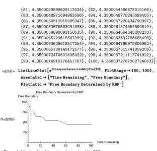
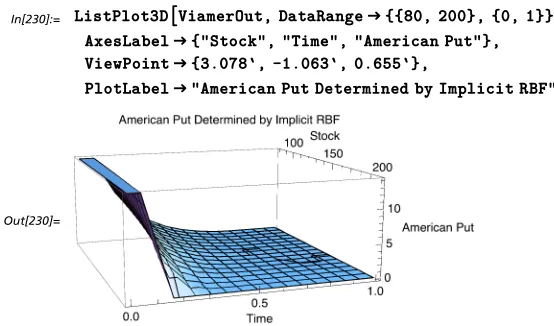
· Optimal Exercise Boundary for the American Put

Furthermore, these programs can now be used to efficiently determine the diffi-cult numerical problem of the moving free boundary for the American option. The concept of the free boundary is that it is the function FBHtL that describes the point at time t where for values of St >FBt the stock price is not so small as to warrant early exercise, and it remains better to hold onto the option, so that it behaves like the European option and satisfies the Black|Scholes PDE of equa-tion (2). However, if St§FBt, then the stock has become sufficiently small as to warrant immediate exercise. On the boundary the value of the option is the exer-cise price resulting in the equation

(25) VHFBHtL, tL=UHyHtL, tL=K-FBHtL = K-eyHtL_.

Consider the time tn=T-nDt; then at that time UHyn,tnL=K-eyn and FHynL=UHyn,tnL-K+eyn =_{0. We now define these F}H_yL _functions.

In[220]:= ClearAllF1, F2, F4, Fi;

F1y_, n_Integer:U1Amery, nK y_;

F2y_, n_Integer:U2Amery, nK y_;

F4y_, n_Integer:U4Amery, nK y_;

Fiy_, n_Integer:UiAmery, nK y_;

In[225]:= OffFindRoot::"lstol"

To check that the zero function FHy,nL is working properly, we use FindRoot, starting at y0=logHKL.

In[226]:= y. FindRootFiy, M,y, LogK, AccuracyGoal10, WorkingPrecision20, MaxIterations300

Out[226]= 4.3500072767206089575

At time tn =T when n=0, FBHTL=K and hence yHTL=logHKL. For successive values of n, we move further back in time to the present and Fi@y,nD determines those values yn such that logHynL=FBHtnL. This procedure is implemented using

NestList, in which successive solutions are used as the starting point for the next evaluation of the FindRoot function.

Evaluation of Financial Options Using Radial Basis Functions in Mathematica 353

At time tn =T when n=0, FBHTL=K and hence yHTL=logHKL. For successive values of n, we move further back in time to the present and Fi@y,nD determines those values yn such that logHynL=FBHtnL. This procedure is implemented using

NestList, in which successive solutions are used as the starting point for the next evaluation of the FindRoot function.

In[227]:= exerciseBdryPts  NestList11,

y. FindRootFiy,11,y,2, AccuracyGoal10, WorkingPrecision20, MaxIterations300&,0, LogK, M Out[227]= 0, Log100,1, 4.5561932385336261842,

2, 4.5436871507129802744,3, 4.5234387898578146500,

4, 4.5000071431279923528,5, 4.4999986047562968794,

6, 4.4999970891333575006,7, 4.4977939168859925177,

8, 4.4911976516584216455,9, 4.4814123344580258802,

10, 4.4675186036495674686,

11, 4.4499200992474832487,12, 4.4499941509843673905,

13, 4.4499996810722396164,14, 4.4500022628395216874,

15, 4.4500028801041949433,16, 4.4500036851563828342,

17, 4.4500040255741613136,18, 4.4500044167108636958,

19, 4.4497999597851553456,20, 4.4475529642319670852,

21, 4.4441290417701749413,22, 4.4397703062635811122,

23, 4.4345081974563303855,24, 4.4282537293048573306,

25, 4.4207944459214501354,26, 4.4117589851304339383,

27, 4.4008960897819213631,28, 4.4000309240267231047,

29, 4.4000098918473913176,30, 4.4000045843086320959,

31, 4.3999994779805448553,32, 4.3999990423301953491,

33, 4.3999971892173454803,34, 4.3999975369740232652,

35, 4.3999958752948114178,36, 4.3999959555671765290,

37, 4.3999948864553056755,38, 4.3999945828136903349,

39, 4.3999947408613160717,40, 4.3999944779944486649,

41, 4.3999938860176458550,42, 4.3999941601254691854,

43, 4.3999938666676987319,44, 4.3999934836647549014,

45, 4.3999929725496883359,46, 4.3999931351484446102,

47, 4.3991586818972903929,48, 4.3978013322568408437,

49, 4.3960807398960029235,50, 4.3940728474171419519,

51, 4.3918155079754839831,52, 4.3893266995970437892,

53, 4.3866107962779580188,54, 4.3836630710763167523,

55, 4.3804691705480343044,56, 4.3770099431876408354,

57, 4.3732550897390454802,58, 4.3691648448976707225,

59, 4.3646844449033349648,60, 4.3597333815258148126,

61, 4.3541604046384914749,62, 4.3491198902332688492,

63, 4.3499022166743211253,64, 4.3499546829139412401,

65, 4.3499688309030937187,66, 4.3499795636567580726,

67, 4.3499877501387976394,68, 4.3499899767448375606,

69, 4.3499928790239539119,70, 4.3499962008878066678,

71, 4.3499974597170615801,72, 4.3499987034351720258,

73, 4.3499989643146470757,74, 4.3500001681914532512,

75, 4.3499999076901291465,76, 4.3500017072156979079,

77, 4.3500027240591525012,78, 4.3500031967844006864,

79, 4.3500033453450793815,80, 4.3500041048372897077,

, ,