Review on solving the inverse problem in EEG source analysis

Open Access

Review

Review on solving the inverse problem in EEG source analysis

Roberta Grech

_{, Tracey Cassar*}

_{, Joseph Muscat}

_{, Kenneth P Camilleri}

_,

Simon G Fabri

_{, Michalis Zervakis}

_{, Petros Xanthopoulos}

_,

Vangelis Sakkalis

_{and Bart Vanrumste}

Address: 1_{iBERG, University of Malta, Malta,} 2_{Department of Systems and Control Engineering, Faculty of Engineering, University of Malta, Malta,} 3_{Department of Electronic and Computer Engineering, Technical University of Crete, Crete,} 4_{Institute of Computer Science, Foundation for}

Research and Technology, Heraklion 71110, Greece, 5_{ESAT, KU Leuven, Belgium and} 6_{MOBILAB, IBW, K.H. Kempen, Geel, Belgium}

Email: Roberta Grech - [email protected]; Tracey Cassar* - [email protected]; Joseph Muscat - [email protected]; Kenneth P Camilleri - [email protected]; Simon G Fabri - [email protected]; Michalis Zervakis - [email protected]; Petros Xanthopoulos - [email protected]; Vangelis Sakkalis - [email protected]; Bart Vanrumste - [email protected] * Corresponding author

Abstract

In this primer, we give a review of the inverse problem for EEG source localization. This is intended for the researchers new in the field to get insight in the state-of-the-art techniques used to find approximate solutions of the brain sources giving rise to a scalp potential recording. Furthermore, a review of the performance results of the different techniques is provided to compare these different inverse solutions. The authors also include the results of a Monte-Carlo analysis which they performed to compare four non parametric algorithms and hence contribute to what is presently recorded in the literature. An extensive list of references to the work of other researchers is also provided.

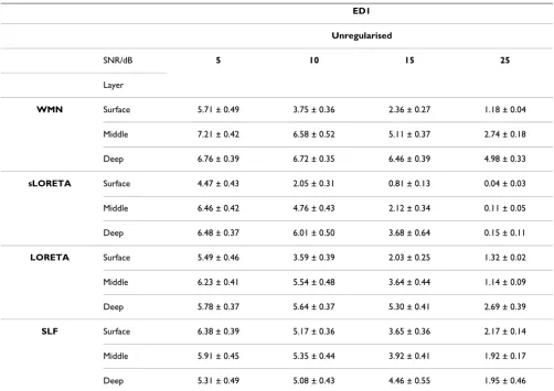
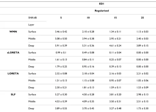
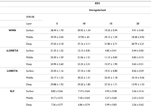
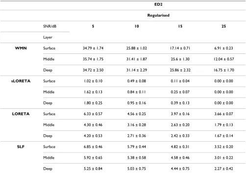
This paper starts off with a mathematical description of the inverse problem and proceeds to discuss the two main categories of methods which were developed to solve the EEG inverse problem, mainly the non parametric and parametric methods. The main difference between the two is to whether a fixed number of dipoles is assumed a priori or not. Various techniques falling within these categories are described including minimum norm estimates and their generalizations, LORETA, sLORETA, VARETA, S-MAP, ST-MAP, Backus-Gilbert, LAURA, Shrinking LORETA FOCUSS (SLF), SSLOFO and ALF for non parametric methods and beamforming techniques, BESA, subspace techniques such as MUSIC and methods derived from it, FINES, simulated annealing and computational intelligence algorithms for parametric methods. From a review of the performance of these techniques as documented in the literature, one could conclude that in most cases the LORETA solution gives satisfactory results. In situations involving clusters of dipoles, higher resolution algorithms such as MUSIC or FINES are however preferred. Imposing reliable biophysical and psychological constraints, as done by LAURA has given superior results. The Monte-Carlo analysis performed, comparing WMN, LORETA, sLORETA and SLF, for different noise levels and different simulated source depths has shown that for single source localization, regularized sLORETA gives the best solution in terms of both localization error and ghost sources. Furthermore the computationally intensive solution given by SLF was not found to give any additional benefits under such simulated conditions.

Published: 7 November 2008

Journal of NeuroEngineering and Rehabilitation 2008, 5:25 doi:10.1186/1743-0003-5-25

Received: 3 June 2008 Accepted: 7 November 2008

This article is available from: http://www.jneuroengrehab.com/content/5/1/25

© 2008 Grech et al; licensee BioMed Central Ltd.

1 Introduction

Over the past few decades, a variety of techniques for non-invasive measurement of brain activity have been devel-oped, one of which is source localization using electroen-cephalography (EEG). It uses measurements of the voltage potential at various locations on the scalp (in the order of microvolts (μV)) and then applies signal processing tech-niques to estimate the current sources inside the brain that best fit this data.

It is well established [1] that neural activity can be mod-elled by currents, with activity during fits being well-approximated by current dipoles. The procedure of source localization works by first finding the scalp potentials that would result from hypothetical dipoles, or more generally from a current distribution inside the head – the forward problem; this is calculated or derived only once or several times depending on the approach used in the inverse problem and has been discussed in the corresponding review on solving the forward problem [2]. Then, in con-junction with the actual EEG data measured at specified positions of (usually less than 100) electrodes on the scalp, it can be used to work back and estimate the sources that fit these measurements – the inverse problem. The accuracy with which a source can be located is affected by a number of factors including head-modelling errors, source-modelling errors and EEG noise (instrumental or biological) [3]. The standard adopted by Baillet et. al. in [4] is that spatial and temporal accuracy should be at least better than 5 mm and 5 ms, respectively.

In this primer, we give a review of the inverse problem in EEG source localization. It is intended for the researcher who is new in the field to get insight in the state-of-the-art techniques used to get approximate solutions. It also pro-vides an extensive list of references to the work of other researchers. The primer starts with a mathematical formu-lation of the problem. Then in Section 3 we proceed to discuss the two main categories of inverse methods: non parametric methods and parametric methods. For the first category we discuss minimum norm estimates and their generalizations, the Backus-Gilbert method, Weighted Resolution Optimization, LAURA, shrinking and mul-tiresolution methods. For the second category, we discuss the non-linear least-squares problem, beamforming approaches, the Multiple-signal Classification Algorithm (MUSIC), the Brain Electric Source Analysis (BESA), sub-space techniques, simulated annealing and finite ele-ments, and computational intelligence algorithms, in particular neural networks and genetic algorithms. In Sec-tion 4 we then give an overview of source localizaSec-tion errors and a review of the performance analysis of the techniques discussed in the previous section. This is then followed by a discussion and conclusion which are given in Section 5.

2 Mathematical formulation

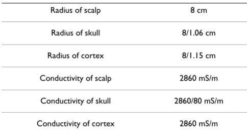
In symbolic terms, the EEG forward problem is that of finding, in a reasonable time, the potential g(r, rdip, d) at an electrode positioned on the scalp at a point having position vector r due to a single dipole with dipole moment d = de_d (with magnitude d and orientation e_d), positioned at rdip (see Figure 1). This amounts to solving Poisson's equation to find the potentials V on the scalp for different configurations of r_dip and d. For multiple dipole sources, the electrode potential would be . Assuming the principle of

super-position, this can be rewritten as

, where g(r,

) now has three components corresponding to the

Cartesian x, y, z directions, d_i = (d_ix, d_iy, d_iz) is a vector con-sisting of the three dipole magnitude components, 'T_' denotes the transpose of a vector, d_i = ||d_i|| is the dipole

magnitude and is the dipole orientation. In

practice, one calculates a potential between an electrode and a reference (which can be another electrode or an average reference).

For N electrodes and p dipoles:

m g _dip

i

i i ( )r =

∑

g r r( , _dip)( _ix, _iy, ) g r r( , ) e

i

iz T

dip i

i i

i d d d i d

∑

∑

r_dipi

e d

d

i i

i

=

A three layer head model

Figure 1

where i = 1, ..., p and j = 1, ..., N. Each row of the gain matrix G is often referred to as the lead-field and it describes the current flow for a given electrode through each dipole position [5].

For N electrodes, p dipoles and T discrete time samples:

where M is the matrix of data measurements at different times m(r, t) and D is the matrix of dipole moments at dif-ferent time instants.

In the formulation above it was assumed that both the magnitude and orientation of the dipoles are unknown. However, based on the fact that apical dendrites produc-ing the measured field are oriented normal to the surface [6], dipoles are often constrained to have such an orienta-tion. In this case only the magnitude of the dipoles will vary and the formulation in (2a) can therefore be re-writ-ten as:

where D is now a matrix of dipole magnitudes at different time instants. This formulation is less underdetermined than that in the previous structure.

Generally a noise or perturbation matrix n is added to the system such that the recorded data matrix M is composed of:

M = GD + n. (4)

Under this notation, the inverse problem then consists of

finding an estimate of the dipole magnitude matrix given the electrode positions and scalp readings M and using the gain matrix G calculated in the forward prob-lem. In what follows, unless otherwise stated, T = 1 with-out loss of generality.

3 Inverse solutions

The EEG inverse problem is an ill-posed problem because for all admissible output voltages, the solution is non-unique (since p >> N) and unstable (the solution is highly sensitive to small changes in the noisy data). There are var-ious methods to remedy the situation (see e.g. [7-9]). As regards the EEG inverse problem, there are six parameters that specify a dipole: three spatial coordinates (x, y, z) and three dipole moment components (orientation angles (θ,

φ) and strength d), but these may be reduced if some con-straints are placed on the source, as described below.

Various mathematical models are possible depending on the number of dipoles assumed in the model and whether one or more of dipole position(s), magnitude(s) and ori-entation(s) is/are kept fixed and which, if any, of these are assumed to be known. In the literature [10] one can find the following models: a single dipole with time-varying unknown position, orientation and magnitude; a fixed number of dipoles with fixed unknown positions and ori-entations but varying amplitudes; fixed known dipole positions and varying orientations and amplitudes; varia-ble number of dipoles (i.e. a dipole at each grid point) but with a set of constraints. As regards dipole moment con-straints, which may be necessary to limit the search space for meaningful dipole sources, Rodriguez-Rivera et al. [11] discuss four dipole models with different dipole moment constraints. These are (i) constant unknown dipole moment; (ii) fixed known dipole moment orientation and variable moment magnitude; (iii) fixed unknown dipole moment orientation, variable moment magnitude; (iv) variable dipole moment orientation and magnitude.

There are two main approaches to the inverse solution: non-parametric and parametric methods. Non-parametric optimization methods are also referred to as Distributed Source Models, Distributed Inverse Solutions (DIS) or Imaging methods. In these models several dipole sources with fixed locations and possibly fixed orientations are distributed in the whole brain volume or cortical surface.

m r

r

g r r g r r

g r r = ⎡ ⎣ ⎢ ⎢ ⎢ ⎤ ⎦ ⎥ ⎥ ⎥ = m m N dip dip N di p ( ) ( ) ( , ) ( , ) ( ,

1 1 1 1

#

"

# % #

pp N dipp p p

d

d 1

1 1

) " ( , )

#

g r r

e e ⎡ ⎣ ⎢ ⎢ ⎢ ⎢ ⎤ ⎦ ⎥ ⎥ ⎥ ⎥ ⎡ ⎣ ⎢ ⎢ ⎢ ⎤ ⎦ ⎥ ⎥ ⎥ (1) M r r r r

G r r = ⎡ ⎣ ⎢ ⎢ ⎢ ⎤ ⎦ ⎥ ⎥ ⎥ =

m m T

m _N m _N T

j dipi

( , ) ( , )

( , ) ( , )

({ , }

11 1

1 " # % # " )) , , , , d d d d T

p p p T p

1 1 1 1 1

1 e e e e " # % # " ⎡ ⎣ ⎢ ⎢ ⎢ ⎤ ⎦ ⎥ ⎥ ⎥ (2a)

=G r r({ ,_{j dip}})D

i (2b)

M

g r r e g r r e

g r r e g r r e

=

( , ) ( , )

( , ) ( , )

1 1 1

1 1

1

dip dip p

N dip N dip

p

p

"

# % #

" _{pp p}

d d ⎡ ⎣ ⎢ ⎢ ⎢ ⎢ ⎤ ⎦ ⎥ ⎥ ⎥ ⎥ ⎡ ⎣ ⎢ ⎢ ⎢ ⎤ ⎦ ⎥ ⎥ ⎥ 1 # (3a) = ⎡ ⎣ ⎢ ⎢ ⎢ ⎤ ⎦ ⎥ ⎥ ⎥ G r r({ , , })e

, ,

, ,

j dip i

T

p p T

i

d d

d d

1 1 1

1

"

# % #

"

(3b)

=G r r({ ,j dipi, })ei D (3c)

ˆ

As it is assumed that sources are intracellular currents in the dendritic trunks of the cortical pyramidal neurons, which are normally oriented to the cortical surface [6], fixed orientation dipoles are generally set to be normally aligned. The amplitudes (and direction) of these dipole sources are then estimated. Since the dipole location is not estimated the problem is a linear one. This means that in Equation 4, { } and possibly e_i are determined

beforehand, yielding large p >> N which makes the prob-lem underdetermined. On the other hand, in the paramet-ric approach few dipoles are assumed in the model whose location and orientation are unknown. Equation (4) is solved for D, { } and e_i, given M and what is known

of G. This is a non-linear problem due to parameters { }, e_i appearing non-linearly in the equation.

These two approaches will now be discussed in more detail.

3.1 Non parametric optimization methods

Besides the Bayesian formulation explained below, there are other approaches for deriving the linear inverse oper-ators which will be described, such as minimization of expected error and generalized Wiener filtering. Details are given in [12]. Bayesian methods can also be used to estimate a probability distribution of solutions rather than a single 'best' solution [13].

3.1.1 The Bayesian framework

In general, this technique consists in finding an estimator of x that maximizes the posterior distribution of x given the measurements y [4,12-15]. This estimator can be writ-ten as

where p(x | y) denotes the conditional probability density of x given the measurements y. This estimator is the most probable one with regards to measurements and a priori

considerations.

According to Bayes' law,

The Gaussian or Normal density function

Assuming the posterior density to have a Gaussian distri-bution, we find

where z is a normalization constant called the partition function, Fα(x) = U1(x) + αL(x) where U1(x) and L(x) are

energy functions associated with p(y | x) and p(x) respec-tively, and α(a positive scalar) is a tuning or regulariza-tion parameter. Then

If measurement noise is assumed to be white, Gaussian and zero-mean, one can write U₁(x) as

U₁(x) = ||Kx - y||2

where K is a compact linear operator [7,16] (representing the forward solution) and ||.|| is the usual L₂ norm. L(x) may be written as U_s(x) + U_t(x) where U_s(x) introduces spatial (anatomical) priors and U_t(x) temporal ones [4,15]. Combining the data attachment term with the prior term,

This equation reflects a trade off between fidelity to the data and spatial/temporal smoothness depending on the

α.

In the above, p(y | x) ∝ exp(-XT_{.X) where X = Kx - y. More} generally, p(y | x) ∝ exp(-Tr(XT_.σ-1_{.X)), where} σ-1 _{is the}

data covariance matrix and 'Tr' denotes the trace of a matrix.

The general Normal density function

Even more generally, p(y | x) ∝ exp(-Tr((X - μ)T_.σ-1_.(X

-μ))), where μis the mean value of X. Suppose R is the var-iance-covariance matrix when a Gaussian noise compo-nent is assumed and Y is the matrix corresponding to the measurements y. The R-norm is defined as follows:

Non-Gaussian priors

Non-Gaussian priors include entropy metrics and L_p

norms with p < 2 i.e. L(x) = ||x||_p.

Entropy is a probabilistic concept appearing in informa-tion theory and statistical mechanics. Assuming x ∈ Rn consists of positive entries x_i > 0, i = 1, ..., n the entropy is defined as

r_dipi

r_dip

i

r_dipi

ˆ

x

ˆ max[ ( | )]

x x y

x

= p

p p p

p

( | ) ( | ) ( ) ( ) .

x y y x x

y =

p p p

p

F z

p

( | ) ( ) ( | ) ( )

exp[ ( )] / ( )

x y x y x

y

x y

= = − a

ˆ min( ( )).

x x

x

= F_a

ˆ min( ( )) min(|| || ( )).

x x Kx y x

x x

= F_a = − 2+aL

where > 0 is a is a given constant. The information

contained in x relative to is the negative of the entropy. If it is required to find x such that only the data Kx = y is used, the information subject to the data needs to be min-imized, that is, the entropy has to be maximized. The mathematical justification for the choice L(x) = - (x) is that it yields the solution which is most 'objective' with respect to missing information. The maximum entropy method has been used with success in image restoration problems where prominent features from noisy data are to be determined.

As regards L_p norms with p < 2, we start by defining these

norms. For a matrix A, where a_ij are

the elements of A. The defining feature of these prior mod-els is that they are concentrated on images with low aver-age amplitude with few outliers standing out. Thus, they are suitable when the prior information is that the image contains small and well localized objects as, for example, in the localization of cortical activity by electric measure-ments.

As p is reduced the solutions will become increasingly sparse. When p = 1 [17] the problem can be modified slightly to be recast as a linear program which can be solved by a simplex method. In this case it is the sum of the absolute values of the solution components that is minimized. Although the solutions obtained with this norm are sparser than those obtained with the L₂ norm, the orientation results were found to be less clear [17]. Another difference is that while the localization results improve if the number of electrodes is increased in the case of the L₂ approach, this is not the case with the L₁

approach which requires an increase in the number of grid points for correct localization. A third difference is that while both approaches perform badly in the presence of noisy data, the L₁ approach performs even worse than the

L₂ approach. For p < 1 it is possible to show that there exists a value 0 <p < 1 for which the solution is maximally sparse. The non-quadratic formulation of the priors may be linked to previous works using Markov Random Fields [18,19]. Experiments in [20] show that the L₁ approach demands more computational effort in comparision with

L₂ approaches. It also produced some spurious sources

and the source distribution of the solution was very differ-ent from the simulated distribution.

Regularization methods

Regularization is the approximation of an ill-posed prob-lem by a family of neighbouring well-posed probprob-lems. There are various regularization methods found in the lit-erature depending on the choice of L(x). The aim is to find the best-approximate solution xδof Kx = y in the situation that the 'noiseless data' y are not known precisely but that only a noisy representation yδwith ||yδ- y|| ≤δis availa-ble. Typically yδwould be the real (noisy) signal. In gen-eral, an is found which minimizes

Fα(x) = ||Kx - yδ||2 + αL(x).

In Tikhonov regularization, L(x) = ||x||2 _{so that an is}

found which minimizes

Fα(x) = ||Kx - yδ||2 + α||x||2.

It can be shown (in Appendix) that

where K* is the adjoint of K. Since (K*K + αI)-1_{K* =} K*(KK* + αI)-1 _{(proof in Appendix),}

Another choice of L(x) is

L(x) = ||Ax||2 ₍₅₎

where A is a linear operator. The minimum is obtained when

In particular, if A = ∇ where ∇ is the gradient operator, then = (K*K + α∇T∇₎-1_{K*y. If A =} Δ_{B, where} Δ_{is the}

Laplacian operator, then = (K*K + αB*ΔTΔ_B)-1_K*y.

The regularization parameter αmust find a good compro-mise between the residual norm ||Kx - yδ|| and the norm of the solution ||Ax||. In other words it must find a bal-ance between the perturbation error in y and the regulari-zation error in the regularized solution.

( )x = − log

∗ ⎛

⎝ ⎜ ⎜

⎞

⎠ ⎟ ⎟ =

∑

xi

i i

n

1

x_i∗

xi∗



|| || | |

,

A _{p ij} p

i j

p _a

=

∑

xad

x_ad

x_{a d}d( ) =(K K∗ +aI)−1K y∗ d

xa dd( ) =K KK∗( ∗+aI)−1yd.

x_{a d}d_{( )}=(K K∗ +aA A∗ )−1K y∗ (6)

x_{a d}d_{( )}

Various methods [7-9] exist to estimate the optimal regu-larization parameter and these fall mainly in two catego-ries:

1. Those based on a good estimate of |||| where is the noise in the measured vector yδ.

2. Those that do not require an estimate of ||||.

The discrepancy principle is the main method based on ||||. In effect it chooses αsuch that the residual norm for the regularized solution satisfies the following condition:

||Kx - yδ|| = ||||

As expected, failure to obtain a good estimate of will yield a value for αwhich is not optimal for the expected solu-tion.

Various other methods of estimating the regularization parameter exist and these fall mainly within the second category. These include, amongst others, the

1. L-curve method

2. General-Cross Validation method

3. Composite Residual and Smoothing Operator (CRESO)

4. Minimal Product method

5. Zero crossing

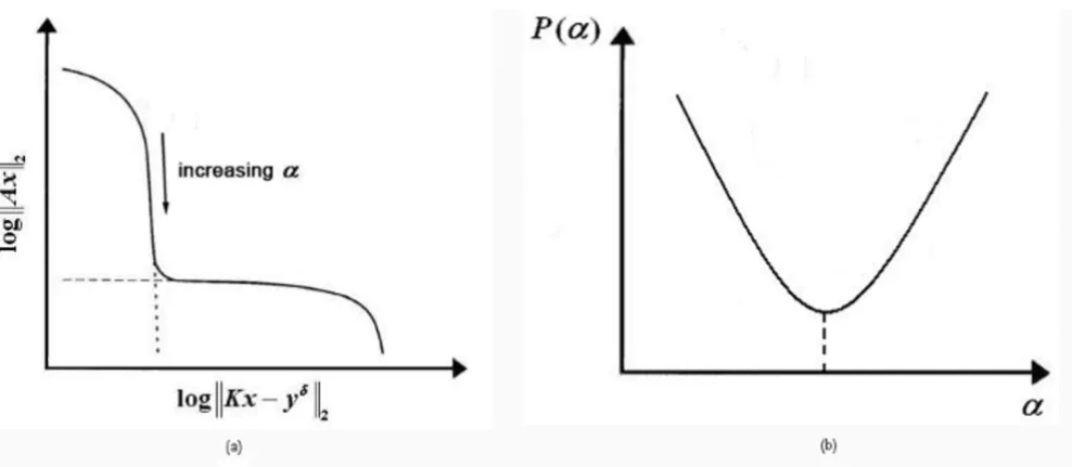
The L-curve method [21-23] provides a log-log plot of the semi-norm ||Ax|| of the regularized solution against the corresponding residual norm ||Kx - yδ|| (Figure 2a). The resulting curve has the shape of an 'L', hence its name, and it clearly displays the compromise between minimizing these two quantities. Thus, the best choice of alpha is that corresponding to the corner of the curve. When the regu-larization method is continuous, as is the case in Tikhonov regularization, the L-curve is a continuous curve. When, however, the regularization method is dis-crete, the L-curve is also discrete and is then typically rep-resented by a spline curve in order to find the corner of the curve.

Similar to the L-curve method, the Minimal Product method [24] aims at minimizing the upper bound of the solution and the residual simultaneously (Figure 2b). In this case the optimum regularization parameter is that corresponding to the minimum value of function P which gives the product between the norm of the solution and the norm of the residual. This approach can be adopted to both continuous and discrete regularization.

P(α) = ||Ax(α)||.||Kx(α) - yδ||

Another well known regularization method is the Gener-alized Cross Validation (GCV) method [21,25] which is based on the assumption that y is affected by normally distributed noise. The optimum alpha for GCV is that cor-responding to the minimum value for the function G:

Methods to estimate the regularization parameter

Figure 2

where T is the inverse operator of matrix K. Hence the numerator measures the discrepancy between the esti-mated and measured signal yδwhile the denominator measures the discrepancy of matrix KT from the identity matrix.

The regularization parameter as estimated by the Com-posite Residual and Smoothing Operator (CRESO) [23,24] is that which maximizes the derivative of the dif-ference between the residual norm and the semi-norm i.e. the derivative of B(α):

B(α) = α2_||Ax(α_)||2 _{- ||Kx(}α_{) - y}δ_||2 ₍₇₎

Unlike the other described methods for finding the regu-larization parameter, this method works only for continu-ous regularization such as Tikhonov.

The final approach to be discussed here is the zero-cross-ing method [23] which finds the optimum regularization parameter by solving B(α) = 0 where B is as defined in Equation (7). Thus the zero-crossing is basically another way of obtaining the L-curve corner.

One must note that the above estimators for are the

same as those that result from the minimization of ||Ax|| subject to Kx = y. In this case x = K(*)_(KK(*)₎-1_{y where K}(*)

= (AA*)-1_{K* is found with respect to the inner product} 77x, y88 = 7Ax, Ay8. This leads to the estimator,

x = (A*A)-1_K*(K(AA*)-1_K*)-1_y

which, if regularized, can be shown to be equivalent to (6).

As regards the EEG inverse problem, using the notation used in the description of the forward problem in Section

??, the Bayesian methods find an estimate of D such that

where

As an example, in [26] one finds that the linear operator

A in Equation (5) is taken to be a matrix A whose rows

represent the averages (linear combinations) of the true sources. One choice of the matrix A is given by

In the above equation, the subscripts p, q are used to indi-cate grid points in the volume representing the brain and the subscripts k, m are used to represent Cartesian coordi-nates x, y and z (i.e. they take values 1,2,3), d_pq represents the Euclidean distances between the pth and qth grid points. The coefficients w_j can be used to describe a col-umn scaling by a diagonal matrix while σ_i controls the spatial resolution. In particular, if σi → 0 and wj = 1 the minimum norm solution described below is obtained.

In the next subsections we review some of the most com-mon choices for L(D).

Minimum norm estimates (MNE)

Minimum norm estimates [5,27,28] are based on a search for the solution with minimum power and correspond to Tikhonov regularization. This kind of estimate is well suited to distributed source models where the dipole activity is likely to extend over some areas of the cortical surface.

L(D) = ||D||2

or

The first equation is more suitable when N > p while the second equation is more suitable when p > N. If we let

T_MNE be the inverse operator GT_(GGT ₊ α_I

N)-1, then TMNEG is called the resolution matrix and this would ideally the identity matrix. It is claimed [5,27] that MNEs produce very poor estimation of the true source locations with both the realistic and sphere models.

A more general minimum-norm inverse solution assumes that both the noise vector n and the dipole strength D are normally distributed with zero mean and their covariance matrices are proportional to the identity matrix and are denoted by C and R respectively. The inverse solution is given in [14]:

G Tr

= −

−

|| ( ) ||

( ( ))

Kx y

I KT

a d 2

2

x_{a d}d_{( )}

ˆ

D

ˆ _{min( ( ))}

D= UD

U( ) ||D = M−GD||_R2 +aL( ).D

A A

w k m

ij p k q m

j

dpq i

=

= =

− + − +

− 3 1 3 1

2 2

( ) , ( )

/

exp s for and zero otherwiise

ˆ _{( )}

D_MNE = G GT +aI_p −1G MT

ˆ _{( )}

DMNE =GT GGT +aIN −1M

ˆ _{( )}

R_ij can also be taken to be equal to σ_iσ_jCorr(i, j) where is the variance of the strength of the ith dipole and Corr(i,

j) is the correlation between the strengths of the ith and jth dipoles. Thus any a priori information about correlation between the dipole strengths at different locations can be used as a constraint. R can also be taken as

where is such that it is

large when the measure ζi of projection onto the noise subspace is small. The matrix C can be taken as σ2_{I if it is}

assumed that the sensor noise is additive and white with constant variance σ2_{. R can also be constructed in such a}

way that it is equal to UUT _{where U is an orthonormal set} of arbitrary basis vectors [12]. The new inverse operator using these arbitrary basis functions is the original for-ward solution projected onto the new basis functions.

Weighted minimum norm estimates (WMNE)

The Weighted Minimum Norm algorithm compensates for the tendency of MNEs to favour weak and surface sources. This is done by introducing a 3p × 3p weighting matrix W:

or

W can have different forms but the simplest one is based on the norm of the columns of the matrix G: W = Ω^I₃, where ^ denotes the Kronecker product and Ωis a

diago-nal p × p matrix with

, for β= 1, ..., p.

MNE with FOCUSS (Focal underdetermined system solution) This is a recursive procedure of weighted minimum norm estimations, developed to give some focal resolution to linear estimators on distributed source models [5,27,29,30]. Weighting of the columns of G is based on the mag nitudes of the sources of the previous iteration. The Weighted Minimum Norm compensates for the lower gains of deeper sources by using lead-field normalization.

where i is the index of the iteration and W_i is a diagonal matrix computed using

, j ∈ [1, 2, ..., p] is a diagonal matrix for

deeper source compensation. G(:, j) is the jth column of

G. The algorithm is initialized with the minimum norm

solution , that is,

,

where (n) represents the nth element of vector . If

continued long enough, FOCUSS converges to a set of concentrated solutions equal in number to the number of electrodes.

The localization accuracy is claimed to be impressively improved in comparison to MNE. However, localization of deeper sources cannot be properly estimated. In addi-tion to Minimum Norm, FOCUSS has also been used in conjunction with LORETA [31] as discussed below.

Low resolution electrical tomography (LORETA)

LORETA [5,27] combines the lead-field normalization with the Laplacian operator, thus, gives the depth-com-pensated inverse solution under the constraint of smoothly distributed sources. It is based on the maximum smoothness of the solution. It normalizes the columns of

G to give all sources (close to the surface and deeper ones) the same opportunity of being reconstructed. This is better than minimum-norm methods in which deeper sources cannot be recovered because dipoles located at the surface of the source space with smaller magnitudes are prive-leged. In LORETA, sources are distributed in the whole inner head volume. In this case, L(D) = ||ΔB.D||2 _{and B =} Ω^I₃ is a diagonal matrix for the column normalization of G.

or

Experiments using LORETA [27] showed that some spuri-ous activity was likely to appear and that this technique was not well suited for focal source estimation.

LORETA with FOCUSS [31]

This approach is similar to MNE with FOCUSS but based on LORETA rather than MNE. It is a combination of LORETA and FOCUSS, according to the following steps: s_i2

R R_{ii jj}(Corr i j( , )) R_ii f

i

=

( )

z

L

WMNE T T T

( ) || ||

( )

D WD

D G G W W G M

=

= + −

2

1 a

(8)

ˆ _{( ) ( ( ) )}

D_WMNE = W WT −1GT G W WT −1GT +aI_N −1M

Ωbb a a

a b b

= ⋅

=

∑

1

ˆ _{( )}

|

D_{FOCUSS i} =W W G_{i i}T T GW W G_{i i}T T +aI_N −1M (9)

Wi =w Wi i−1 diag (Di−1) (10)

w

G i =diag

(

)

ˆ

D_MNE

W0=diag(DMNE)=diag(D0( ),1 D0( ),...,2 D0(3p))

ˆ

D₀ Dˆ₀

ˆ _{( )}

D_LOR = G GT +aBΔ ΔT B −1G MT

ˆ _{( ) ( ( ) )}

1. The current density is computed using LORETA to get

.

2. The weighting matrix W is constructed using (10), the initial matrix being given by

, where

(n) represents the nth element of vector .

3. The current density is computed using (9).

4. Steps (2) and (3) are repeated until convergence.

Standardized low resolution brain electromagnetic tomography Standardized low resolution brain electromagnetic tom-ography (sLORETA) [32] sounds like a modification of LORETA but the concept is quite different and it does not use the Laplacian operator. It is a method in which local-ization is based on images of standardized current den-sity. It uses the current density estimate given by the

minimum norm estimate and standardizes it by using its variance, which is hypothesized to be due to the actual source variance S_D = I_3p, and variation due to noisy

measurements = αI_N. The electrical potential

vari-ance is S_M = GS_DGT _{+ and the variance of the} esti-mated current density is

. This is

equiv-alent to the resolution matrix T_MNEG. For the case of EEG with unknown current density vector, sLORETA gives the following estimate of standardized current density power:

where ∈R3 × 1 _{is the current density estimate at the}

lth voxel given by the minimum norm estimate and [ ]_ll

∈R3 × 3 _{is the lth diagonal block of the resolution matrix}

. It was found [32] that in all noise free simulations,

although the image was blurred, sLORETA had exact, zero error localization when reconstructing single sources, that is, the maximum of the current density power estimate coincided with the exact dipole location. In all noisy sim-ulations, it had the lowest localization errors when com-pared with the minimum norm solution and the Dale method [33]. The Dale method is similar to the sLORETA method in that the current density estimate given by the minimum norm solution is used and source localization

is based on standardized values of the current density mates. However, the variance of the current density esti-mate is based only on the measurement noise, in contrast to sLORETA, which takes into account the actual source variance as well.

Variable resolution electrical tomography (VARETA)

VARETA [34] is a weighted minimum norm solution in which the regularization parameter varies spatially at each point of the solution grid. At points at which the regulari-zation parameter is small, the source is treated as concen-trated When the regularization parameter is large the source is estimated to be zero.

where L is a nonsingular univariate discrete Laplacian, L₃

= L ^I_{3 × 3}, where ^ denotes the Kronecker product, W is a certain weight matrix defined in the weighted minimum norm solution, Λ is a diagonal matrix of regularizing parameters, and parameters τand αare introduced. τ con-trols the amount of smoothness and αthe relative impor-tance of each grid point. Estimators are calculated iteratively, starting with a given initial estimate D₀ (which

may be taken to be ), Λ_i is estimated from D_{i - 1}, then

D_i from Λ_i until one of them converges.

Simulations carried out with VARETA indicate the neces-sity of very fine grid spacing [34].

Quadratic regularization and spatial regularization (S-MAP) using dipole intensity gradients

In Quadratic regularization using dipole intensity gradi-ents [4], L(D) = ||∇D||2 _{which results in a source estimator}

given by

or

The use of dipole intensity gradients gives rise to smooth variations in the solution.

Spatial regularization is a modification of Quadratic regu-larization. It is an inversion procedure based on a non-quadratic choice for L(D) which makes the estimator become non-linear and more suitable to detect intensity jumps [27].

ˆ

DLOR

W0=diag(DLOR)=diag(D0( ),1 D0( ),...,2 D0(3p))

ˆ

D₀ Dˆ₀

ˆ

D_i

ˆ

DMNE

S_Mnoise

SMnoise

S_Dˆ =TMNES T_M MNET =G GGT[ T +aIN]−1G

ˆ _{{[ ] }} ˆ

, ˆ ,

DTMNE l S_D ll −1DMNE l (11)

ˆ

, D_{MNE l}

S_Dˆ

S_Dˆ

ˆ _{arg min(|| || || . . || || . ln( ) || )}

,

D M GD L W D L

D

VAR= − + + −

LL

L

L LL

2 3

2 _t2 _a 2

ˆ

D_LOR

ˆ _{( )}

DQR= G GT + ∇ ∇a T −1G MT

ˆ _{( ) ( ( ) ) )}

where N_v = p × N_n and N_n is the number of neighbours for

each source j, ∇D_|v is the vth element of the gradient vector

and . K_v = α_v × β_v where α_v

depends on the distance between a source and its current neighbour and β_v depends on the discrepancy regarding orientations of two sources considered. For small gradi-ents the local cost is quadratic, thus producing areas with smooth spatial changes in intensity, whereas for higher

gradients, the associated cost is finite: Φ_v(u) ≈ , thus

allowing the preservation of discontinuities. The estima-tor at the ith iteration is of the form

where Θ is a p by N matrix depending on G and priors computed from the previous source estimate .

Spatio-temporal regularization (ST-MAP)

Time is taken into account in this model whereby the assumption is made that dipole magnitudes are evolving slowly with regard to the sampling frequency [4,15]. For a

measurement taken at time t, assuming that and may be very close to each other means that the orthogonal

projection of on the hyperplane perpendicular

to is 'small'. The following nonlinear equation is obtained:

where

is a weighted Laplacian and

with

is the projector onto .

Spatio-temporal modelling

Apart from imposing temporal smoothness constraints, Galka et. al. [35] solved the inverse problem by recasting it as a spatio-temporal state space model which they solve by using Kalman filtering. The computational complexity of this approach that arises due to the high dimensionality of the state vector was addressed by decomposing the model into a set of coupled low-dimensional problems requiring a moderate computational effort. The initial state estimates for the Kalman filter are provided by LORETA. It is shown that by choosing appropriate dynamical models, better solutions than those obtained by the instantaneous inverse solutions (such as LORETA) are obtained.

3.1.2 The Backus-Gilbert method

The Backus-Gilbert method [5,7,36] consists of finding an approximate inverse operator T of G that projects the EEG data M onto the solution space in such a way that the esti-mated primary current density = TM, is closest to the real primary current density inside the brain, in a least square sense. This is done by making the 1 × p vector

(u, v = 1, 2, 3 and γ= 1, ..., p) as close as

pos-sible to where δis the Kronecker delta and I_γis the

γth column of the p × p identity matrix. G_v is a N × p matrix derived from G in such a way that in each row, only the elements in G corresponding to the vth direction are kept. The Backus-Gilbert method seeks to minimize the spread of the resolution matrix R, that is to maximize the resolv-ing power. The generalized inverse matrix T optimizes, in a weighted sense, the resolution matrix.

We reproduce the discrete version of the Backus-Gilbert problem as given in [5]:

under the normalization constraint: . 1p is a p

× 1 matrix consisting of ones.

One choice for the p × p diagonal matrix is:

where v_i is the position vector of grid point i in the head model. Note that the first part of the functional to be

min-L _{v v}

n Nv

( )D = (∇D_|)

=

∑

1

Φv( )u =u +⎛_{K v}u ⎝⎜

⎞ ⎠⎟ ⎡

⎣ ⎢ ⎢

⎤

⎦ ⎥ ⎥

2 ₁ 2

K_v2

ˆ _{( , ( ˆ ))}

D_i =ΘG LD_i−1 M

ˆ

Di−1

ˆ

Dt−1 Dˆt

ˆ

Dt E_Dˆ_t

−1 ⊥

ˆ

Dt−1

G GT t Pt Pt Dt G MT t T

+a(Δ +b ⊥₋1 ⊥₋1) =

Δt x T

x t

x T

x yT yt y

= −∇ B ∇ ∇ − ∇ B ∇

B_xt =diag.[b_xt | ]_{k k=1,...,p}

b x t k

x t k

x t

k

| ( | )

| .

= ′ ∇

∇

Φ D

D

2

P_t⊥₋₁ E

t

ˆ D₋1 ⊥

ˆ

D_BG

R_uvT_g =T G_uT_{g v}

duvIgT

min{[ ] [ ] ( ) }

Tu I G T W G T T G G T

u T

u T BG uT u vu uT v vT u v

I g

g − g g g − g + −d g g =

1

1 3 3

∑

T G 1uTg u p =1

W_gBG

imized attempts to ensure correct position of the localized dipoles while the second part ensures their correct orien-tation.

The solution for this EEG Backus-Gilbert inverse operator is:

where:

'†_{' denotes the Moore-Penrose pseudoinverse.}

3.1.3 The weighted resolution optimization

An extension of the Backus-Gilbert method is called the Weighted Resolution Optimization (WROP) [37]. The modification by Grave de Peralta Menendez is cited in [5].

is replaced by where

The second part of the functional to be minimzed is replaced by

where

αGdeP _and βGdeP _{are scalars greater than zero. In practice this} means that there is more trade off between correct locali-zation and correct orientation than in the above Backus-Gilbert inverse problem.

In this case the inverse operator is:

In [5] five different inverse methods (the class of instanta-neous, 3D, discrete linear solutions for the EEG inverse problem) were analyzed and compared for noise-free measurements: minimum norm, weighted minimum norm, Backus-Gilbert, weighted resolution optimization (WROP) and LORETA. Of the five inverse solutions tested,

only LORETA demonstrated the ability of correct localiza-tion in 3D space.

The WROP method is a family of linear distributed solu-tions including all weighted minimum norm solusolu-tions. As particular cases of the WROP family there are LAURA [26,38], a local autoregressive average which includes physical constraints into the solutions and EPI-FOCUS [38] which is a linear inverse (quasi) solution, especially suitable for single, but not necessarily point-like genera-tors in realistic head models. EPIFOCUS has demon-strated a remarkable robustness against noise.

LAURA

As stated in [39] in a norm minimization approach we make several assumptions in order to choose the optimal mathematical solution (since the inverse problem is underdetermined). Therefore the validity of the assump-tions determine the success of the inverse solution. Unfor-tunately, in most approaches, criteria are purely mathematical and do not incorporate biophysical and psychological constraints. LAURA (Local AUtoRegressive Average) [40] attempts to incorporate biophysical laws into the minimum norm solution.

According to Maxwell's laws of electromagnetic field, the strength of each source falls off with the reciprocal of the cubic distance for vector fields and with the reciprocal of the squared distance for potential fields. LAURA method assumes that the electromagnetic activity will occur according to these two laws.

In LAURA the current estimate is given by the following equation:

The W_j matrix is constructed as follows:

1. Denote by the vicinity of each solution point defined as the hexahedron centred at the point and com-prising at most = 26 points.

2. For each solution point denote by Nk the number of neighbours of that point and by d_ki the Euclidean distance from point k to point i (and vice versa).

3. Compute the matrix A using e_i = 2 for scalar fields and

e_i = 3 for vector fields

and

T E L

L E L

u

u u

u T

u u

g g

g =

†

†

L G 1 E C F

C G W G F G G

u u p u u uv v

v

u u BG uT v v vT

= = + −

= =

=

∑

, ( ) ,

, .

g g

g g

d 1

1 3

W_gBG W₁GdeP_g

[W₁GdeP_g ]_ll =||v_l−v_g||2+bGdeP.

(1 )

1 3

2 −

=

∑

v

uT v GdeP vT u

T G W G T

[W2GdePg ]ll =||vl−vg ||2+bGdeP+aGdeP,

T_u GdeP G W_u GdePG_uT _uv G W_v GdePG_vT G I_u

v

g =b g + −d g g

=

∑

{ ₁ ( ) ₂ } .

1 3

1

ˆ _{( )}

D_LAURA=W G_j T GW G_j−1 T +aI_N −1M

_i

max

A max

Ni d

ii ki

e

k i

i

= −

∈

∑

4. The weight matrix W_j is defined by:

W_j = PT_P

where:

P = W_mA ^I₃

where I₃ is the 3 × 3 identity matrix and ^ denotes the Kro-necker product. W_m is a diagonal matrix formed by the mean of the norm of the three columns of the lead field matrix associated with the ith point.

3.1.4 Shrinking methods and multiresolution methods

By applying suitable iterations to the solution of a distrib-uted source model, a concentrated source solution may be obtained. Ways of performing this are explained in the next section.

S-MAP with iterative focusing

This modified version [27] of Spatial Regularization is dedicated to the recovery of focal sources when the spatial sampling of the cortical surface is sparse. The source space dimension is reduced by iterative focusing on the regions that have been previously estimated with significant dipole activity. An energy criterion is used which takes into consideration both the source intensities and its con-tribution to data:

E = 2E_c + E_a

where E_c measures the contribution of every dipole source to the data and E_a is an indicator of dipole relative magni-tudes. Sources with energy greater than a certain threshold are selected for the next iteration. The estimator at the ith iteration is given by

where G_i is the column-reduced version of G and Θis a p_i ≤p by N matrix depending on the G_i and priors computed

from the previous source estimate . A similar

approach was used in [31] where the source region was contracted several times but at each iteration, LORETA was used to estimate the source tomography.

Shrinking LORETA-FOCUSS

This algorithm combines the ideas of LORETA and FOCUSS and makes iterative adjustments to the solution space in order to reduce computation time and increase

source resolution [?, 20]. Starting from the smooth LORETA solution, it enhances the strength of some prom-inent dipoles in the solution and diminishes the strength of other dipoles. The steps [20] are as follows:

1. The current density is computed using LORETA to get

.

2. The weighting matrix W is constructed using (10), its initial value being given by

.

3. The current density is computed using (9).

4. (Smoothing operation) The prominent nodes (e.g. those with values larger than 1% of the maximum value) and their neighbours are retained. The current density val-ues on these prominent nodes and their neighbours are readjusted by smoothing, the new values being given by

where r_l is the position vector of the lth node and s_l is the number of neighbouring nodes around the lth node with distance equal to the minimum inter-node distance d.

5. (Shrinking operation) The corresponding elements in

and G are retained and the matrix M = D is com-puted.

6. Steps (2) to (5) are repeated until convergence.

7. The solution of the last iteration before smoothing is the final solution.

Steps (4) and (5) are stopped if the new solution space has fewer nodes than the number of electrodes or the solution of the current iteration is less sparse than that estimated by the previous iteration. Once steps (4) and (5) are stopped, the algorithm becomes a FOCUSS process. Results [20] using simulated noiseless data show that Shrinking LORETA-FOCUSS is able to reconstruct a three-dimensional source distribution with smaller localization and energy errors compared to Weighted Minimum Norm, the L1 approach and LORETA with FOCUSS. It is

also 10 times faster than LORETA with FOCUSS and sev-eral hundred times faster than the L₁ approach.

Standardized shrinking LORETA-FOCUSS (SSLOFO)

SSLOFO [41] combines the features of high resolution (FOCUSS) and low resolution (WMN, sLORETA)

meth-Aik dki ei

= − −

ˆ _{( , ( ˆ )).}

D_i =QQG_i−1 L D_i−1 M

ˆ

D_i−1

ˆ

DLOR

W0=diag(DLOR)=diag(D0( ),1 D0( ),...,2 D0(3p))

ˆ

Di

1 1

sl l u u u r r d

l u

+ +

⎛

⎝ ⎜ ⎜

⎞

⎠ ⎟

⎟ ∀ − =

∑

ˆ ( ) ˆ ( ) || ||

D D under constraint

ˆ

ods. In this way, it can extract regions of dominant activity as well as localize multiple sources within those regions. The procedure is similar to that in Shrinking LORETA-FOCUSS with the exception of the first three steps which are:

1. The current density is computed using sLORETA to get

.

2. The weighting matrix W is constructed using (10), its initial value being given by

.

3. The current density is computed using (9). The

power of the source estimation is then normalized as

where and [R_i]_ll is the

lth diagonal block of matrix R_i.

In [41], SSLOFO reconstructed different source configura-tions better than WMN and sLORETA. It also gave better results than FOCUSS when there were many extended sources. A spatio-temporal version of SSLOFO is also given in [41]. An important feature of this algorithm is that the temporal waveforms of single/multiple sources in the simulation studies are clearly reconstructed, thus ena-bling estimation of neural dynamics directly from the cor-tical sources. Neither Shrinking LORETA-FOCUSS nor FOCUSS are able to accurately reconstruct the time series of source activities.

Adaptive standardized LORETA/FOCUSS (ALF)

The algorithms described above require a full computa-tion of the matrix G. On the other hand, ALF [42] requires only 6%–11% of this matrix. ALF localizes sources from a sparse sampling of the source space. It minimizes forward computations through an adaptive procedure that increases source resolution as the spatial extent is reduced. The algorithm has the following steps:

1. A set of successive decimation ratios on the set of possi-ble sources is defined. These ratios determine successively higher resolutions, the first ratio being selected so as to produce a targeted number of sources chosen by the user and the last one produces the full resolution of the model.

2. Starting with the first decimation ratio, only the corre-sponding dipole locations and columns in G are retained.

3. sLORETA (Equation(11)) is used to achieve a smooth solution. The source with maximum normalized power is selected as the centre point for spatial refinement in the next iteration, in which the next decimation ratio is applied. Successive iterations include sources within a spherical region at successively higher resolutions.

4. Steps 2 and 3 are repeated until the last decimation ratio is reached. The solution produced by the final itera-tion of sLORETA is used as initializaitera-tion of the FOCUSS algorithm. Standardization (Equation(12)) is incorpo-rated into each FOCUSS iteration as well.

5. Iterations are continued until there is no change in solution.

It is shown in [42] that the localization accuracy achieved is not significantly different than that obtained when an exhaustive search in a fully-sampled source space is made. A multiresolution framework approach was also used in [15]. At each iteration of the algorithm, the source space on the cortical surface was scanned at higher spatial reso-lution such that at every resoreso-lution but the highest, the number of source candidates was kept constant.

3.1.5 Summary

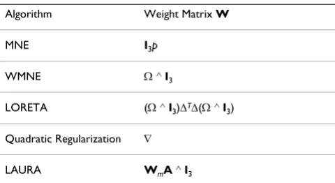
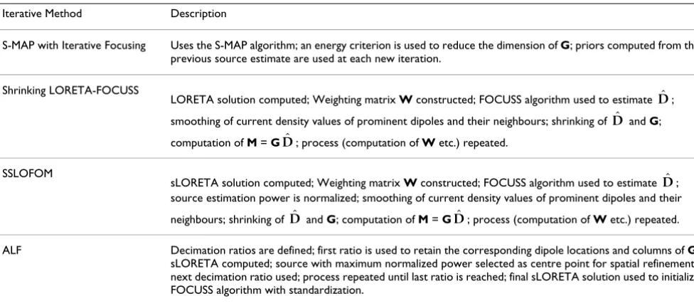
Refering to Equation (8), Table 1 summarizes the differ-ent weight matrices used in the algorithms. Refering to Subsection 3.1.4, Table 2 summarizes the steps involved in the different iterative methods which were discussed.

3.2 Parametric methods

Parametric Methods are also referred to as Equivalent Cur-rent Dipole Methods or Concentrated Source or Spatio-Temporal Dipole Fit Models. In this approach, a search is made for the best dipole position(s) and orientation(s). The models range in complexity from a single dipole in a spherical head model, to multiple dipoles (up to ten or more) in a realistic head model. Dynamic models take into consideration dipole changes in time as well. Con-ˆ

D_sLOR

W₀=diag(D_sLOR)=diag(D₀( ),1 D₀( ),...,2 D₀(3p))

ˆ

D_i

ˆ ( ){[ ] } ( )

D_iT l R_{i ll} −1D_i l (12)

Ri =W W Gi iT T(GW Wi iT +aI G)

Table 1: Summary of weighting strategies for the various non-parametric methods. For definition of notation, refer to the respective subsection.

Algorithm Weight Matrix W

MNE I3p

WMNE Ω^I₃

LORETA (Ω^I3)ΔTΔ(Ω^I3)

Quadratic Regularization ∇

straints on the dipole orientations, whether fixed or varia-ble, may be made as well.

3.2.1 The non-linear least-squares problem

The best location and dipole moment (six parameters in all for each dipole) are usually obtained by finding the global minimum of the residual energy, that is the L₂

-norm ||V_in - V_model||, where V_model ∈RN _{represents the}

elec-trode potentials with the hypothetical dipoles, and V_in ∈ RN _{represents the recorded EEG for a single time instant.} This requires a non-linear minimization of the cost func-tion ||M - G({r_j, })D|| over all of the parameters

( , D). Common search methods include the gradient,

downhill or standard simplex search methods (such as Nelder-Mead) [43-46], normally including multi-starts, as well as genetic algorithms and very time-consuming sim-ulated annealing [45,47,48]. In these iterative processes, the dipolar source is moved about in the head model while its orientation and magnitude are also changed to obtain the best fit between the recorded EEG and those produced by the source in the model. Each iterative step requires several forward solution calculations using test dipole parameters to compare the fit produced by the test dipole with that of the previous step.

3.2.2 Beamforming approaches

Beamformers are also called spatial filters or virtual sen-sors. They have the advantage that the number of dipoles must not be assumed a priori. The output y(t) of the beam-former is computed as the product of a 3 × N (each

Carte-sian axis is considered) spatial filtering matrix WT _with

m(t), the N × 1 vector representing the signal at the array at a given time instant t associated with a single dipole source, i.e. y(t) = WT_{m(t). This output represents the} neu-ronal activity of each dipole d in the best possible way at a given time t.

In beamforming approaches [6], the signals from the elec-trodes are filtered in such a way that only those coming from sources of interest are maintained. If the location of interest is r_dip, the spatial filter should satisfy the following constraints:

where G(r) = [g(r, e_x), g(r, e_y), g(r, e_z)] is the N × 3 forward matrix for three orthogonal dipoles at location r having orientation vectors e_x, e_y and e_z respectively, I is the 3 × 3 identity matrix and δrepresents a small distance.

In linearly constrained minimum variance (LCMV) beam-forming [49], nulls are placed at positions corresponding to interfering sources, i.e. neural sources at locations other than r_dip (so δ= 0). The LCMV problem can be written as:

where Cy = E[yyT] = WTCmW and Cm = E[mmT] is the signal

covariance matrix estimated from the available data. This means that the beamformer minimizes the output energy

WT_C

mW under the constraint that only the dipole at rdip is active at that time. Minimization of variance optimally allocates the stop band response of the filter to attenuate

rdipi

r_dip

i

W r G r I r r

0 r r

T dip

dip dip

( ) ( ) , || ||

, || ||

=⎧_⎨⎪ −₋ ≤_> ⎩⎪

d d

min ( ) ( ) ( )

WT Tr Cy W r G r I

T

dip dip

subject to =

Table 2: Steps involved in the iterative methods

Iterative Method Description

S-MAP with Iterative Focusing Uses the S-MAP algorithm; an energy criterion is used to reduce the dimension of G; priors computed from the previous source estimate are used at each new iteration.

Shrinking LORETA-FOCUSS

LORETA solution computed; Weighting matrix W constructed; FOCUSS algorithm used to estimate ;

smoothing of current density values of prominent dipoles and their neighbours; shrinking of and G; computation of M = G ; process (computation of W etc.) repeated.

SSLOFOM

sLORETA solution computed; Weighting matrix W constructed; FOCUSS algorithm used to estimate ;

source estimation power is normalized; smoothing of current density values of prominent dipoles and their

neighbours; shrinking of and G; computation of M = G ; process (computation of W etc.) repeated.

ALF Decimation ratios are defined; first ratio is used to retain the corresponding dipole locations and columns of G;

sLORETA computed; source with maximum normalized power selected as centre point for spatial refinement; next decimation ratio used; process repeated until last ratio is reached; final sLORETA solution used to initialize FOCUSS algorithm with standardization.

ˆ

D

ˆ

D

ˆ

D

ˆ

D

ˆ