Discrete-Element bonded-particle Sea Ice model DESIgn, version 1.3a – model description and implementation

(1)

www.geosci-model-dev.net/9/1219/2016/ doi:10.5194/gmd-9-1219-2016

Discrete-Element bonded-particle Sea Ice model DESIgn,

version 1.3a – model description and implementation

Agnieszka Herman

Institute of Oceanography, University of Gdansk, Pilsudskiego 46, 81-378 Gdynia, Poland Correspondence to: Agnieszka Herman ([email protected])

Received: 31 May 2015 – Published in Geosci. Model Dev. Discuss.: 15 July 2015 Revised: 7 March 2016 – Accepted: 16 March 2016 – Published: 1 April 2016

Abstract. This paper presents theoretical foundations, nu-merical implementation and examples of application of the two-dimensional Discrete-Element bonded-particle Sea Ice model – DESIgn. In the model, sea ice is represented as an assemblage of objects of two types: disk-shaped “grains” and semi-elastic bonds connecting them. Grains move on the sea surface under the influence of forces from the atmosphere and the ocean, as well as interactions with surrounding grains through direct contact (Hertzian contact mechanics) and/or through bonds. The model has an experimental option of tak-ing into account quasi-three-dimensional effects related to the space- and time-varying curvature of the sea surface, thus enabling simulation of ice breaking due to stresses resulting from bending moments associated with surface waves. Ex-amples of the model’s application to simple sea ice defor-mation and breaking problems are presented, with an analy-sis of the influence of the basic model parameters (“micro-scopic” properties of grains and bonds) on the large-scale response of the modeled material. The model is written as a toolbox suitable for usage with the open-source numeri-cal library LIGGGHTS. The code, together with full techni-cal documentation and example input files, is freely available with this paper and on the Internet.

1 Introduction

Sea ice cover in polar and subpolar seas is a complex assem-blage of ice blocks of various sizes, thicknesses, ages, struc-tures and properties resulting from their genesis, typically consisting of multiple cycles of partial melting, (re)freezing and mechanical deformation resulting from the action of ex-ternal agents (wind, waves, solar radiation, etc.) and from

interactions with surrounding ice. In favorable conditions, the ice blocks may join (freeze) to form larger blocks (ice floes), behaving like semi-rigid bodies, so that the deforma-tion of ice is localized, limited to narrow shear and com-pression zones. This type of ice cover is characteristic of the compact, central Arctic ice pack. Close to the ice edge, ex-tensive breaking primarily caused by ocean waves produces ice behaving as a polydisperse granular material composed of individual, relatively small floes of various diameters. In all cases, many important aspects of sea ice dynamics are directly related to its discrete, discontinuous nature. Con-sequently, although some of the large-scale effects of those processes can be parametrized in continuum sea ice models, mechanisms underlying them can be investigated and under-stood only by means of models that properly take into ac-count the fundamental physics.

(2)

range of these mechanisms is much wider than this list sug-gests (see further Sect. 2.2) and is only beginning to be ap-preciated as new observational and computational techniques provide new insights into sea ice physics and dynamics.

The Discrete-Element, bonded-particle Sea Ice model – DESIgn – presented here has been developed as a tool for studying the processes mentioned above at the floe level, with hope that it will help to deepen our understanding of ice dynamics at different scales, and possibly to develop parametrizations of relevant processes for continuum mod-els.

This paper presents the theoretical background, underlying assumptions and equations of the model, its numerical imple-mentation and examples of applications to sea ice problems. The model is an extension of the earlier versions described in Herman (2013a, b). The paper is accompanied by the model code and a full technical documentation, so that it can be freely used and modified by anyone, as described in the last section. A full, very detailed description of all equations used in the model is provided, even if some of them are standard in discrete-element models (DEMs) – for the sake of complete-ness and in order to make it easier for users inexperienced in DEMs to configure and run their own simulations. The main purpose of the modeling results presented here is the verifi-cation of the model’s consistency and its new features rather than validation against observational data, which will be pre-sented in further works.

The model is two-dimensional (2-D), but it enables one to take into account some wave-related effects, i.e., stresses re-sulting from flexural moments acting on sea ice when surface waves are present. It can be applied to a wide range of sea ice types, although it is worth stressing here that the word “gran-ular” in the present context describes macroscopic, large-scale ice properties, i.e., the fact that it is composed of in-dividual ice floes. It does not refer in any way to smaller-scale material structures at the level of (groups of) ice crys-tals. Also, in view of specific assumptions underlying the model (e.g., the above-mentioned two-dimensionality), it is not suitable for early stages of sea ice formation, like frazil and grease ice; pancake ice can be regarded as a rough lower limit of the model validity in terms of floe size. On the other hand, although the model was designed for sea ice, it can be applied to other 2-D materials composed of disk-shaped grains.

The paper is structured as follows. The next section con-tains a short review of previous attempts to account for the granular nature of sea ice in numerical models of its dynam-ics. Section 3 begins with the general concept and underly-ing assumptions of the model proposed here, followed by the presentation of the equations. The mechanics of grains and bonds is discussed in Sects. 4 and 5, followed in Sect. 6 by the presentation of the types of internal forcing implemented in the present model version. The numerical implementa-tion of the model is described in Sect. 7. Modeling results illustrating the most important aspects of the bond-related

model behavior are presented in Sect. 8, followed by a dis-cussion of possible directions of the further model develop-ment in Sect. 9.

2 Modeling granular effects in sea ice dynamics – a brief review

2.1 Sea ice floe-size distribution

From the point of view of processes analyzed here, one of the most important properties of sea ice is the FSD. Since the seminal paper of Rothrock and Thorndike (1984), obser-vations from various parts of the world showed that typical FSDs are very wide and can be well approximated by a power law (e.g., Lytle et al., 1997; Holt and Martin, 2001; Paget et al., 2001; Toyota and Enomoto, 2002; Inoue et al., 2004; Toyota et al., 2006; Lu et al., 2008; Steer et al., 2008; Toy-ota et al., 2011). However, only a few attempts have been made to create models that would explain the observed vari-ation of the FSD shapes, including the values of the expo-nent of the distribution and deviations from the power law occurring in certain situations. The validity and range of ap-plicability of the proposed statistical models (Herman, 2010; Toyota et al., 2011; Perovich and Jones, 2014) remain to be assessed. Power laws are produced by a very wide range of models, including very simple models of breaking, mak-ing the selection of a proper model and the identification of mechanisms that are important in any particular real-world situation a challenge.

2.2 Parametrization of granular effects in continuum models

A number of parametrizations have been developed to im-prove the performance of continuum sea ice models in situ-ations when granular effects have a significant influence on the large-scale sea ice behavior. One group of parametriza-tions is related to the so-called collisional rheology, describ-ing stress in fragmented sea ice due to inelastic collisions between floes, relevant especially in the MIZ. In the existing collisional rheology models, stress is calculated from the av-erage collision frequency and momentum transferred during collisions, assuming uniform distribution of the floes on the sea surface and either constant (Shen et al., 1984, 1986; Lep-päranta et al., 1989) or variable floe sizes (Lu et al., 1989). Although the models proved useful in reproducing some as-pects of sea ice flow in the MIZ (Feltham, 2005), collisional rheology is very rarely taken into account in ice modeling, presumably partly because the rather unrealistic assumptions on which it is based tend to underestimate the contribution of collisional effects to the total stress.

(3)

neighboring grains. Their model relates the effective angle of friction of sea ice – its macroscopic property – to the mi-croscopic angle of friction characterizing the material. Im-plemented in a continuum sea ice model of the Arctic, the parametrization permits ice concentrations lower than 1 in the central ice pack, mimicking the lead-opening processes.

Steele (1992) proposed a parametrization of the lateral-melting rate in sea ice composed of separate floes of a given mean diameter. A number of studies concentrate on parametrization of floe-related effects on the effective skin and drag coefficients over fragmented sea ice (Steele et al., 1989; Lu et al., 2011; Lüpkes et al., 2012, and references therein), as well as on various aspects of sea ice–wave in-teractions in the MIZ. For example, Dumont et al. (2011) formulated the first combined strain and stress failure crite-ria for ice breaking in a flexural mode due to the action of waves. Their results were used by Williams et al. (2013a, b) to formulate a wave–ice interaction model for the MIZ, in which waves break the ice, thus determining the maximum floe size and the FSD, and in turn the FSD is used to esti-mate the wave attenuation term in the wave energy balance equation.

Following the well-established theory describing the evo-lution of the ice-thickness distribution in continuum sea ice models, analogous equations for the floe-size distribution (Zhang et al., 2015) and for the joint floe-size and thickness distribution (Horvat and Tziperman, 2015) have been pro-posed recently, thus providing a general framework within which advection, lateral freezing and melting, as well as ridg-ing and fragmentation processes can be parametrized, mak-ing continuum models more suitable for the MIZ.

2.3 Discrete-element methods in sea ice modeling Although continuum models remain a standard tool for sim-ulating sea ice dynamics, especially at large scales, a num-ber of discrete-element models have been developed in recent decades in which sea ice is represented as an assemblage of interacting objects (“particles”); although the models share the same underlying idea, they differ in terms of the shape and properties of their building blocks, details of the contact mechanics formulations, parametrization of physical pro-cesses not explicitly accounted for in the model (e.g., ridg-ing), as well as numerical algorithms used to solve the model equations. Some models combine an Eulerian, grid-based approach typical for continuum models with a Lagrangian, particle-based approach used in DEMs – examples include particle-in-cell (PIC) models (Flato, 1993; Huang and Sav-age, 1998), distributed-mass/discrete-floe (DMDF) models (Rheem et al., 1997; Fujisaki et al., 2007) or smoothed-particle hydrodynamics (SPH) models (Gutfraind and Sav-age, 1997a, b, 1998; Li et al., 2014). In PIC and DMDF, ice floes are represented by individual particles, advected in a Lagrangian manner based on velocities obtained from mo-mentum equations solved on a fixed grid. By contrast, in

SPH models Lagrangian particles represent sets of discrete ice floes. The SPH models with Mohr–Coulomb rheology, implemented within the viscous-plastic approach of Hibler, proved particularly useful for sea ice problems with strong deformation zones and/or complicated geometry (Gutfraind and Savage, 1997a, b, 1998). It is worth stressing that the authors use a DEM model, conceptually very similar to the one proposed here (Savage, 1995; Sayed et al., 1995), to verify their SPH model – they treat DEM as “a very useful tool for the determination of the most appropriate rheology to describe ice as a continuum”. Their DEM model is 2-D, based on disk-shaped particles, and takes into account con-tact forces as well as air and water drag as external forcing to calculate the motion of each particle in the system.

(4)

Finally, the works by Herman (2011, 2012, 2013a, b, c) present results obtained with DEMs of increasing complex-ity that have led to the development of the model presented here: from a simple event-driven molecular-dynamics type of model suitable for low-concentration sea ice (Herman, 2011, 2012), to a DEM including a contact mechanics model suit-able for studying deformation of a compact ice cover (Her-man, 2013a, b, c). The common focus of these works has been on strong polydispersity (i.e., heterogeneity of sizes) of sea ice floes and the role that it plays in sea ice dynamics, in-cluding cluster formation of ice floes and stress transmission in ice under shear deformation.

3 Bonded-particle discrete-element sea ice model 3.1 General model concept

The sea ice model proposed in this work describes the mo-tion and interacmo-tions of two types, or classes, of objects. Fol-lowing the nomenclature used in similar models of rocks and soils, we will refer to those two types of objects as “grains” or “particles”, and “bonds”. (In the documentation of the nu-merical libraries on which the nunu-merical model is based, the terms “atoms” and “bonds” are used independently of the type of those objects; see Sect. 7.) Together they form a het-erogeneous granular material with large-scale macroscopic behavior depending on the mechanical properties of its indi-vidual parts interacting at a “microscopic” scale. In rock me-chanics, where bonds represent the cement filling spaces be-tween grains of sedimentary or crystalline rocks, such mod-els have been shown to reproduce a wide range of observed rock behavior, including crack formation and propagation, damage accumulation, and dilational effects (Potyondy and Cundall, 2004; Cho et al., 2007; Asadi et al., 2012; Bahaad-dini et al., 2013). Similarly, bonded-particle models are suc-cessfully used to study the behavior of cohesive soils, as well as calving and fracturing of glaciers (Åström et al., 2013).

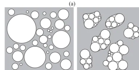
In the context of sea ice, we define the particles as disk-shaped sea ice blocks moving within a 2-D space represent-ing the sea surface. The bonds form when the neighborrepresent-ing disks freeze together. In other words, bonds represent new, usually thinner ice filling cracks, leads and other open spaces between thicker ice blocks. Throughout this paper, sets of bonded particles will be called floes – similarly as in Hop-kins and Thorndike (2006), who treated ice floes as groups of frozen discrete elements of their model. Depending on the context and the purpose of a particular model configura-tion, the ice disks may be interpreted as elementary “building blocks” of sea ice floes, or as floes themselves (Fig. 1). In the first case, useful for example in studies of floe formation and evolution of the floe-size distribution (FSD), it is reasonable to base the simulation on a very large number of disks with sizes much smaller than the expected floe size. In the second case, the FSD may be regarded as given, and its influence on

(a) (b)

Figure 1. Two approaches to the usage of grains and bonds in

DE-SIgn: without bonds, when ice floes are identical to grains and the FSD is prescribed (a); with bonds, when ice floes are assemblages of bonded grains and the FSD is obtained as a solution (b).

the sea ice behavior analyzed in a way similar to that in Her-man (2011, 2012, 2013a, b), whose model is a special case of the one presented here.

There are two essentially independent mechanisms of in-teractions between neighboring particles. The first, based on repulsive and frictional forces between particles, requires that they are in direct contact with each other. The second requires that the particles are connected with an elastic bond. Crucially, whereas forces are transmitted in both cases, bonds are also able to transmit momentum. Another substantial dif-ference between the two interaction types results from the fact that bonds have a certain tensile strength. Consequently, if they are present in a material, it attains a tensile strength at a macroscopic level as well.

From the point of view of sea ice modeling, the bonded-particle approach has a number of important advantages and provides an opportunity to overcome several drawbacks of the existing models. In particular, the model is suitable for arbitrary ice concentrationA, from a compact ice cover at

A'1 to very loose ice composed of freely drifting floes atA1. The same equations describe short pairwise col-lisions and semi-permanent contact between floes. Also, the model is suitable for both a rapid flow regime with rela-tively large ice velocities and for quasi-static deformation in a compact ice pack. Furthermore, non-cylindrical floes can be modeled as bonded assemblages of disk-shaped elemen-tary particles, so that the model equations are still solved for simple, centrally symmetric objects, without the need to cal-culate and store their orientation – which is not the case in models based, e.g., on polygonal elements, which require complicated algorithms for calculating grain overlap, force momenta and orientation (see, e.g., Hopkins, 1992, 2004).

(5)

between pairs of grains located closer to each other than a specified distance (see the technical documentation). 3.2 Basic definitions and assumptions

Let us consider an ensemble of N disk-shaped ice grains, each with a constant mass density ρ, and with variable thicknesshi and radiiri, fori=1, . . ., N. To make a clear

distinction between the horizontal and vertical dimensions, we adopt the following notation in a Cartesian coordi-nate system: [xi, zi] = [x1,i, x2,i, zi]denotes the position of

the center of the ith disk, [ui, uz,i] = [u1,i, u2,i, uz,i] the

translational velocity of its mass center, and [ωi, ωz,i] = [ω1,i, ω2,i, ωz,i]its angular velocity. As already mentioned,

the model is two-dimensional, with some effects related to surface waves included. Precisely, this means thatzi≡0 and uz,i≡0, and the distance between disksiandj is calculated

asδij = kxi−xjk−(ri+rj), i.e., within thex1x2plane. In the

absence of waves, the vertical axes of the disks are perpen-dicular to the horizontal sea surface. If waves are present,zi

anduz,iare still equal to zero; the only change is thatωi6=0

and the deviation of the disks’ axes from the vertical axis are described by a tilt [θi,0] = [θ1,i, θ2,i,0]. For details of the

wave-related effects, see further Sect. 6.3.

The horizontal space _S available to the particles may be unlimited or bounded by rigid walls representing shorelines, concrete structures, etc.; in a general case, they may change their position over time. The motion of the disks within_Sis influenced by (i) the body and surface forces from the ocean and the atmosphere and (ii) the particle–particle and particle– wall interaction forces. For the sake of simplicity and con-ciseness, the particle–wall forces are not included in the equations formulated below (in the model implementation, they are treated in exactly the same way as their particle– particle counterparts, as the contact model used is equally valid for both kinds of contact).

Let_Ci(t )denote the set of all disks in contact with diskiat

a certain time instancet. For eachj∈_C_i, the respective pair-wise contact force will be denoted with Fc,ij. It is convenient

to express this force as a sum of two components, normal and tangential to the plane of contact: Fc,ij,nand Fc,ij,t. The

normal component contributes to the translational motion of disksiandj, and the tangential component to their rotation. The respective torque Mc,ij equals

Mc,ij=rij×Fc,ij,t, (1)

where rij is a vector of lengthri pointing from the center of

diskito the contact point with diskj.

Analogously, let_Bi(t )denote the set of all disks that are

bonded to disk i at time t, and Fb,ij and Mb,ij the

bond-transmitted force and torque, respectively, calculated for all

j ∈_B_i. Again, Fb,ijis a sum of two components, Fb,ij,nand

Fb,ij,t, but the total torque Mb,ijnot only results from Fb,ij,t,

but also includes bending and twisting components, as de-tailed in Sect. 5.2.

Finally, the net external force acting on diski, Fe,i, can be

obtained from the density of surface and body forces, fs,iand

fb,i (measured in N m−2and N m−3, respectively):

Fe,i= Z

Si

fs,ids+ Z

Vi

fb,idv, (2)

whereSi andVi denote the total surface area and volume of

the disk. Analogously, the net moment of those forces is Me,i=

Z

Si

r×fs,ids+ Z

Vi

r×fb,idv, (3)

where r denotes the distance from the disk center. 3.3 Momentum equations for grains

Let us define a unit vector pointing upward, n= [0,0,1], and a 3×3 projection matrix H from the 3-D space to thex1x2

plane:H11=H22=1 and all remaining elements are zero.

By definition, the horizontal position xi and tiltθiare related

to ui andωi, respectively, through

ui=

dxi

dt , (4)

ω_i=dθi

dt . (5)

The general form of the equation describing the translational motion of theith grain is

mi

dui

dt =H 

Fe,i+

X

j∈Ci(t )

Fc,ij,n+ X

j∈Bi(t )

Fb,ij,n 

, (6)

wheremi=πρhiri2 is the mass of the grain andt denotes

time. Analogously, the angular-momentum equations can be written in the form of Euler’s rotation equations for a rigid body:

Ix,i

dωi

dt =(Iz,i−Ix,i)ωz,in× [ωi, ωz]

+H



Me,i+

X

j∈Bi(t )

Mb,ij,t 

, (7)

Iz,i

dωz,i

dt =n· 

Me,i+

X

j∈Ci(t )

Mc,ij+ X

j∈Bi(t )

Mb,ij,t 

. (8)

In the grain-fixed frame of reference, in which these equa-tions are formulated, the inertia tensor is diagonal and its principal values are

Ix1,i=Ix2,i=Ix,i=

1 12mi

3r_i2+h2_i, Iz,i=mi r_i2

(6)

4 Grain–grain contact mechanics

Each of the normal and tangential forces Fc,ij,nand Fc,ij,t is

a sum of two terms. The two normal forces are the repulsive force and the viscoelastic damping force; the tangential force is a sum of the shear force and the damping force. The damp-ing components depend on the relative velocity between the interacting particles. At each time step, the amplitude of the tangential force is limited through the Coulomb friction law:

|Fc,ij,t| ≤µ|Fc,ij,n|, (10)

whereµis the static yield criterion.

The details of the formulation of the contact forces de-pend on the selected contact model and on the geometry of the interacting particles, as described in Sect. S1 of the Sup-plement, which also contains the derivation of the full set of equations used in the present sea ice model. Both alternative formulations available are based on the Hertzian contact me-chanics. Additional details of the Hertzian model in a general context can be found, e.g., in Brilliantov et al. (1996), Zhang and Makse (2005), Schwager (2007) and Zhou (2011). In sea ice studies, (elements of) this model were used, e.g., by Hop-kins and Thorndike (2006), Fortt and Schulson (2011) and Xu et al. (2012).

Notably, in the quasi-3-D version of the model, the con-tact forces are calculated in the same way as in the 2-D ver-sion, i.e., without taking into account the tilt between grains – which amounts to the assumption that the orientations of the axes of symmetry of neighboring grains do not deviate significantly from each other.

5 Elastic bonds 5.1 Bond properties

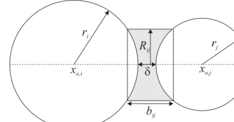
In the following, the bonds are identified by the pair of in-dices of grains that they connect. Each bond, cuboid in shape, is characterized by the following set of properties: thickness

hij; lengthbij; width 2Rij(measured in the direction

perpen-dicular to the line connecting the centers of grainsiandj; see Fig. 2); Young’s modulusEb; ratio of the normal to shear

stiffness λns; tensile strength σt,max; compressive strength

σc,max; shear strengthτmax. In the present model formulation,

Rij=λRmin{ri, rj}, (11)

bij=λb(ri+rj), (12)

where λR∈(0,1], λb∈(0,1] – similarly to Eb, σt,max,

σc,max,τmax– are global parameters, common for all bonds

of a given type (the model enables one to define a number of bond types with different properties). Whenλb=1,

elas-tic deformation is calculated as if it were distributed across grains (as, e.g., in the sea ice model of Hopkins et al., 2004); when λb→0, it is limited to narrow zones at the grains’

r

i

r

j

R

ij

d

x

o,i

x

o,j

b

ij

Figure 2. Geometry of two grains,iandj, connected with a semi-elastic bond.

boundaries. Note that the distance δ between the grains’ edges (Fig. 2) is not included in the calculation ofbij. The

normal and shear stiffness,kn,ijandkt,ij, depends onEband

the bond’s length:

kn,ij= Eb

bij

and kt,ij= kn,ij

λns

. (13)

The moments of inertia of the bond are Ix1,ij=Ix2,ij= Ix,ij=1₆h3_ijRij andIz,ij=2₃hijR_ij3, and the polar moment

of inertiaJij=Ix,ij+Iz,ij.

5.2 Bond mechanics

The forces and torques acting on the grains connected with a bond result from the (finite) relative displacement and rota-tion of those grains; they can be decomposed into axial, tan-gential, bending and twisting components (Obermayr et al., 2013). Similarly to the history effects in the contact model, the force increment during a time period1tcan be calculated based on differences between the grains’ linear and angular velocities,1uij=uj−ui and1ωij=ωj−ωi.

The components of the force due to the relative displace-ment are calculated from a linear elastic material law, in which the force is proportional to the displacement, given by1t 1uij:

Fb,ij,n(t )=γdFb,ij,n(t−1t )+kn,ijSij1t 1uij,n, (14)

Fb,ij,t(t )=γdFb,ij,t(t−1t )+kt,ijSij1t 1uij,t, (15)

whereSij=2Rijhij is the cross-sectional area of the bond, γdis a damping coefficient (preventing spurious oscillations

of the forces), and1uij,nand1uij,t denote components of 1uijnormal and tangential to the plane of contact (or,

equiv-alently, parallel and perpendicular to the bond axis). In the 2-D model, both forces act in the horizontal plane and thus

Fb,ij,t contributes to the grains’ rotation around thezaxis.

(7)

by

Mb,ij,t w(t )=γdMb,ij,t w(t−1t )

−kt,ijJij1t[1ωij,n,0], (16)

Mb,ij,bn(t )=γdMb,ij,bn(t−1t )

−kn,ij1t[Ix,ij1ωij,t, Iz,ij1ωij,z], (17)

where1ωij,n and1ωij,t denote the normal and tangential

components of1ω_ij, respectively.

In total, Mb,ij,t in Eqs. (7) and (8) is given by

Mb,ij,t =rij×Fb,ij,t+Mb,ij,t w+Mb,ij,bn. (18)

In the 2-D version of the model, the twisting moment

Mb,ij,t w≡0 and only the zcomponent of the bending

mo-ment Mb,ij,bn can be different from zero. Note that in

Eqs. (14)–(17), the forces and moments have to be rotated after each time step due to changes in the orientation of the bond.

5.3 Breaking criteria

According to the classical beam theory, the shear stress act-ing on the bond can be calculated as

τb,ij= |Fb,ij,t|

Sij

+|Mb,ij,t w|Rij Jij

. (19)

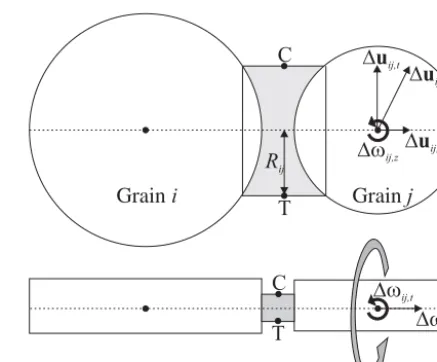
The normal stress reaches its maximum value at the bond peripheries. It has two components, one from the bending moment resulting from the relative rotation of the grains (let-ters “C” and “T” in Fig. 3), and one from the normal force. The bending moment produces tension and compression on the opposite sides of the bond, which may be enhanced or reduced by the normal force depending on its sign. Thus, the maximum tensile and compressive normal stress can be writ-ten as

σt,ij= −

Fb,ij,n Sij

+|HMb,ij,bn|hij Ix,ij

+|n·Mb,ij,bn|Rij Iz,ij

, (20)

σc,ij=

Fb,ij,n Sij

+|HMb,ij,bn|hij Ix,ij

+|n·Mb,ij,bn|Rij Iz,ij

. (21)

In the present version, the bond breaks if at least one of the stress components (Eqs. 19–21) acting on that bond exceeds the bond strength, i.e., if

σt,ij> σt,max or σc,ij> σc,max or τb,ij> τmax. (22)

6 External forcing

In terms of the formulation of forces acting on the grains, the model is very flexible and enables one to specify any com-bination of forces that may be space- and time-varying and depend on the properties of the individual grains (e.g., their mass or size). To make the configuration of the model more

(a)

Duij

T

Duij,t

Duij,n

Dwij,z C

Graini Grainj

Rij

(b)

Dwij,n

Dwij,t T

C

Figure 3. Forces and torques acting on an elastic bond connecting

grainsiandj: top view (a) and side view (b). Letters C and T de-note points where maximum compressive and tensile stress, respec-tively, occurs due to the bending moment caused by1ωij,z in (a)

and1ω_ij,t in (b). Gray curved arrow in (b) denotes the twisting moment associated with1ωij,n.

convenient, formulae describing the forces most relevant to the motion of sea ice on the sea surface have been imple-mented in the code and the corresponding forces can be acti-vated easily by means of simple commands described in the User’s Guide. These forces include the Coriolis force and the skin and form drag due to the wind and surface current. 6.1 The Coriolis force

The Coriolis force acting on theith grain, FC,i, is given as

FC,i= −mifn×ui, (23)

where the Coriolis parameterf=2Zsinφ,Zdenotes the

angular velocity of the Earth, and the latitudeφcan be con-stant or spatially variable. The net torque due to the Coriolis force: MC,i ≡0.

6.2 Wind and surface currents

In most real-world situations, the dominating surface forces acting on sea ice floes are the atmospheric and oceanic skin drag,τha,i andτhw,i, and body drag,τva,i andτvw,i:

τha,i=ρaCha|ua|ua, (24)

τhw,i=ρwChw|uw−ui|(uw−ui), (25)

τva,i=ρaCva|ua|ua, (26)

τvw,i=ρwCvw|uw−ui|(uw−ui), (27)

whereρa and ρw denote the air and water density, ua and

uw are the wind and current velocities, andCha,Chw,Cva,

(8)

the grain. The skin drag acts on the upper and lower sur-faces of the grains, respectively, with the surface area of both equal toπ r_i2. The atmospheric and oceanic body drags,

τva,i and τvw,i, act on the grain’s edges above and below

the water line, respectively. Here we assume that the verti-cal area exposed toτva,iequalsπ rihf,i, and the area exposed

toτvw,iequalsπ ri(hi−hf,i), wherehf,i=hi(ρw−ρ)/ρwis

the grain’s freeboard. In the case of deformed ice, additional drag acting on the slopes of ridges and keels could be taken into account by modifying these expressions. In the present form, the net forces from the atmosphere and the ocean inte-grated over the respective surface areas become

Fa,i=π ri2ρa

Cha+

hi ri

ρw−ρ

ρw

Cva

|ua|ua, (28)

Fw,i=π ri2ρw

Chw+

hi ri ρ ρw Cvw

|uw−ui|(uw−ui). (29)

The net torque ofFa,i equals zero (a direct consequence of

the assumption that the air–ice stress does not depend on the grain’s motion). Because of the dependence ofFw,i on the

disk’s velocity relative to the water, thezcomponent of the torque associated with this force, Mz,w,i, is different from

zero and has a damping effect on the disk’s rotation:

Mz,w,i= −π r_i4

2ρw

Chw+

hi ri ρ ρw Cvw

ωz,i. (30)

6.3 Surface waves 6.3.1 General idea

In the MIZ, as well as in regions with low ice concentra-tions, sea ice is affected by surface waves (wind waves and, most importantly, swell). Flexural stresses related to the cur-vature of the sea surface are one of – or presumably the – dominant factors leading to floe breakup (e.g., Dumont et al., 2011; Williams et al., 2013a). However, these stresses, be-ing related to forces and torques actbe-ing out of the horizontal

x1x2plane, cannot be taken into account in a 2-D model. A

question emerges whether – and how – some of the wave-induced effects can be included in the model without intro-ducing full three-dimensionality, i.e., without having to aban-don the obvious advantage of calculating the floe–floe dis-tances and solving the equations within a 2-D plane.

The wave-related effects available in the present version of the model are under development and should be treated as a starting point for more advanced models. At present, two wave-related processes have been implemented: forces due to the oscillating surface current, and a net moment of buoy-ancy forces due to the time-varying sea surface slope and cur-vature. These two mechanisms tend to be relevant in differ-ent conditions. The alternating convergence and divergence associated with oscillatory motion of the sea surface, and the resulting tensile and compressive stress, influence pancake ice formation and dynamics (Shen et al., 2004). It is generally

significant for relatively small floes, whereas larger ones are affected by the curvature of the sea surface (Dumont et al., 2011).

Obviously, there are a number of other wave-related ef-fects that are very important but not included in the present model. Most crucially, the wave properties have to be pre-scribed – they may be spatially and temporarily variable, but are unaffected by the ice, which means that, for example, wave scattering and reflection at the floes’ edges cannot be taken into account. Similarly, although the tilt of the grains is calculated, this is not the case for their vertical movement. Whereas some of these additional aspects of wave–ice inter-actions can be relatively easily implemented in the type of model described here, others, like for example rafting and ridging during compression, would require either a fully 3-D computation (like in Hopkins and Tuhkuri, 1999) or some kind of parametrization – see the last section for more dis-cussion.

6.3.2 Oscillating surface current

Let us suppose that the sea surface elevationξ=ξ(x, t )is given as a superposition ofNwvpropagating harmonic

deep-water waves:

ξ=

Nwv X

n=1

ancos(kn·x−ωnt+φn)= Nwv X

n=1

ancosϕn, (31)

where an, ωn and φn denote wave amplitude, frequency

and phase, respectively, of the nth component and kn= [k1,n, k2,n,0] is its wavenumber vector. The instantaneous

horizontal velocity uwv,nof water particles at the sea surface

(z=0) associated with that component equals uwv,n=ωnan

kn kn

cosϕn. (32)

After summing the contribution from all elementary waves and averaging over the surface of theith grain, we obtain

uwv,i=

1

π r_i2 Nwv X

n=1

ωnan

kn kn Z

Si

cosϕndS

and finally

uwv,i= Nwv X

n=1

ωnan

kn kn

sin(k1,nri) k1,nri

sin(k2,nri) k2,nri

cosϕn. (33)

The oscillatory current is effective only for small grains and long waves (knri→0) when sin(knri)/(knri)→1. At the

(9)

If the oscillating current is to be taken into account in the model, uwv,i is added to the formula for the current-induced

force (Eq. 29), uw= ¯uw+uwv,i, whereu¯wdenotes the slowly

varying component of the total current. 6.3.3 Wave-induced horizontal torque

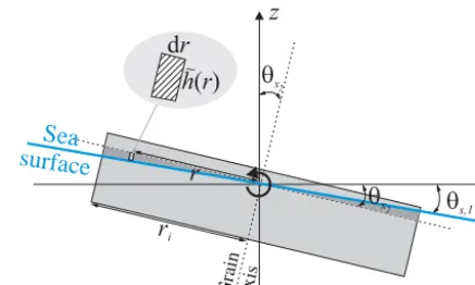
As mentioned above, the presence of waves and the asso-ciated space- and time-varying slope of the sea surface in-duces torque and rotation around the horizontal axes of the ice grains. In the following, an assumption is made that the x components of torque are produced by the unbalanced buoyancy forces acting on a disk if its upper surface is not parallel to the local sea surface, as shown in Fig. 4. It is also assumed for simplicity that exactly half of the disk ex-periences an excess of buoyancy, the other half an excess of gravity (see also Dumont et al., 2011). As defined in Sect. 3.2,θi= [θ1,i, θ2,i,0]denotes the tilt of the disk; i.e., θ1,iandθ2,iare angles between thezaxis and the projection

of the symmetry axis of the disk onto thex1zandx2zplanes,

respectively. Furthermore, let θs,i= [θs,1,i, θs,2,i,0] denote

the mean sea surface slope “under” the disk: tanθs,1,i= ξ(x1,i+ri, x2,i)−ξ(x1,i−ri, x2,i)/(2r) and tanθs,2,i= ξ(x1,i, x2,i+ri)−ξ(x1,i, x2,i−ri)/(2r). The unbalanced

part of the (vertical) buoyancy force acting on an elementary volumeV (r)e at the horizontal distance r=r[cosθ,sinθ,0]

from the grain center (dashed area in Fig. 4) is

Fwv,z,i(r)= ˆρghei(r)rdθdr,

whereehi(r)=βi·r,βi=tan(θi−θs,i), and ρˆequals ρor ρwfor the emerged or submerged part of the grain. Thus, the

total torque, integrated over the disk’s volume, is

Mwv,i= ri

Z

0 2π Z

0

Fb,z,i(r)n×rdθdr,

which gives Mwv,i=

π

4

ρ+ρw

2 gr

4

in×βi. (34)

It should be added as part of Me,i to the right-hand side

of Eq. (7); as the vertical component of Mwv,i equals zero, it

does not contribute to Eq. (8).

For unbonded grains, their angular momentum resulting from Eq. (34), and thus variation of their tilt, depends both on their size and the wave characteristics: they decrease with increasing grain radius and wavelength.

7 The numerical model

The numerical model is based on two libraries designed for effective simulation of large systems of objects inter-acting through a variety of short- or long-range forces:

Grain axis

z

x

1

q

x

q

s,1

Sea

surface

q

x

d

r

h r

~

( )

r

i

2 2

Figure 4. A sketch of a circular grain on a sloping sea surface,

il-lustrating the variables involved in calculation of the wave-induced torque (see text for details).

LAMMPS (Large-scale Atomic/Molecular Massively Par-allel Simulator; Plimpton, 1995, http://lammps.sandia.gov/) and LIGGGHTS (LAMMPS Improved for General Granu-lar and GranuGranu-lar Heat Transfer Simulations; Kloss and Go-niva, 2010, 2011; Kloss et al., 2012, http://www.cfdem.com). The code of the DESIgn model has the form of a tool-box that – thanks to the modular, easily extendable nature of the above libraries – can be incorporated into the stan-dard LIGGGHTS program in a straightforward manner, as described in the attached documentation. Importantly, many changes to the model configuration, including specification of additional forcing types, can be made via configuration files, without modification and recompilation of the code. All information on the availability of the code can be found in Sect. “Code availability” at the end of this paper.

Details regarding the numerical aspects of the model can be found in the User’s Guide (available in the “doc” folder in the attached material) and in the documentation of LAMMPS/LIGGGHTS. DESIgn uses the standard methods of the solution of the governing equations implemented in LIGGGHTS. Therefore, only the most important facts re-garding the numerical aspects of the model are given here.

(10)

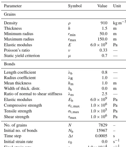
Table 1. Physical and numerical model parameters used in the

ref-erence simulations in Sect. 8.1.

Parameter Symbol Value Unit

Grains

Density ρ 910 kg m−3

Thickness h 1.5 m

Minimum radius rmin 50.0 m

Maximum radius rmax 150.0 m

Elastic modulus E 6.0×109 Pa

Poisson’s ratio ν 0.33 —

Static yield criterion µ 0.7 —

Bonds

Length coefficient λb 0.8 —

Radius coefficient λR 1.0 —

Mean thickness hm 1.0 m

Width of thick. distr. δh 0.0 m

Ratio of normal to shear stiffness λns 2.5 —

Elastic modulus Eb 6.0×109 Pa

Compressive strength σc,max 1.0×106 Pa

Tensile strength σt,max 1.0×105 Pa

Shear strength τmax 1.0×106 Pa

No. of grains N 7829 –

Initial no. of bonds Nb 15967 –

Time step 1t 0.0005 s

Initial strain rate ε0 0.0 s−1

Final strain rate εe 1.0×10−4 s−1

8 Modeling results

All simulations described in Herman (2011, 2012, 2013a, b, c), obtained with older, LAMMPS-based versions of the model, can be reproduced with its present version, with proper model settings. Therefore, the results presented here concentrate on the new model features related to the func-tioning of bonds and to the influence of waves on sea ice. They have been obtained with very simple configurations and can be treated as test cases that verify the model behavior in clearly defined, easily interpretable situations. Both groups of calculations presented below (Sects. 8.1 and 8.2) were per-formed for the so-called reference model setting, as well as for a number of settings differing from the reference ones in terms of one selected parameter, so that the influence of that parameter on the model behavior could be analyzed. The model parameters used in the two reference simulations are listed in Tables 1–3. Simulations similar to those presented below are useful for calibration purposes, as they help to find relationships between the “microscopic” properties of grains and bonds and the desired “macroscopic” properties of sea ice such as its compressive or tensile strength, which in real sea ice varies strongly with changing temperature, ice poros-ity, microstructure, etc. For a summary of material properties of sea ice, see, e.g., Schulson (1999) and Petrovic (2003).

8.1 Sea ice breakup under plane stress

In the first set of simulations, a rectangular sample of com-pact sea ice (densely packed grains with uniform size dis-tribution, fully connected with their neighbors) is subject to a prescribed uniaxial tensile, uniaxial compressive, or shear strain. The strain rate is obtained by setting to zero the veloc-ity of the grains located at the lower boundary of the domain, and moving the grains located at the upper boundary with a specified velocity until terminal failure (see Herman, 2013c, for a similar model configuration without bonds). In all cases the strain rate increased linearly in time fromε0to the

max-imum valueεe. In the great majority of cases, macroscopic

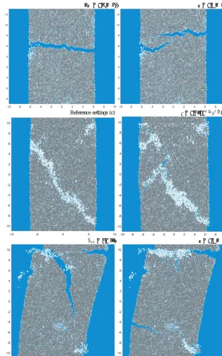
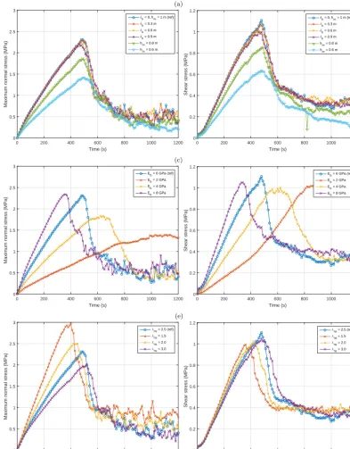
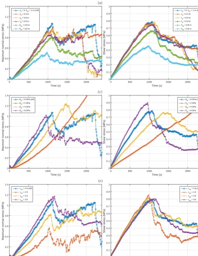
failure of the sample occurred before the end of the simula-tion. Figure 5 shows examples of damage patterns resulting from compressive, tensile and shear deformation. The evolu-tion of the global maximum normal stress and the shear stress under compressive and shear strain is shown in Figs. 6 and 7, respectively. Analogous plots for tensile strain simulations are shown in Fig. S3 in the Supplement.

In all cases, the initial increase in strain results in a fast, ap-proximately linear increase in stress. The rate of the stress ac-cumulation in the material depends on its properties. In par-ticular, it increases with increasing mean bond thicknesshm

and bond Young’s modulusEb(panels a–d in Figs. 6 and 7

and Fig. S3). By contrast, the width of the bond-thickness distribution δh – that is, the spatial inhomogeneity of the

bond thickness – hardly influences the slope of the stress curves. However, it understandably does influence the final damage pattern: for a given value ofhm, higherδhimplies a

larger number of thin, weak bonds distributed throughout the material, and thus more potential spots where breaking can be initialized. Consequently, a more complex damage pat-tern develops, with a larger number of fracture zones with more ragged surfaces. This can be seen even in the simplest configurations, like those in Fig. 5a, b: under tension, a uni-form material tends to break along an approximately straight line, whereas largeδhin situation in panel b resulted in two

competing fractures propagating in opposite directions. Eas-ier initiation of breaking is also responsible for slightly lower macroscopic strength of samples with largerδh(panels a, b

in Figs. 6 and 7 and Fig. S3).

The role ofλns, defined in Eq. (13), is more complex, as

its influence on the macroscopic material behavior depends on the type of deformation. (It is worth stressing that λns

determines the shear stiffnesskt; it has no influence on the

normal stiffnesskn.) Under uniaxial compression, higherkt

stabilizes the bonds and contributes to the overall strength of the material. Under shear strain, varyingλnsmanifests

it-self in very different fracture patterns. Smallλns, i.e., large

kt, produces fracture zones aligned approximately with the

(11)

hm= 0.8 m (a) δh= 0.9 m (b)

Reference settings (c) ε0= 0.3x10−4s−1(d)

λns= 3.0 (e) δh= 0.9 m (f) x

Figure 5. Example damage patterns obtained in simulations of an initially compact sample under uniaxial tensile (a, b), uniaxial

compres-sive (c, d), and shear (e, f) strain. Thick gray lines show the bonds between grains. Model parameters that differed from the reference run are given with each panel. See Figs. S3–S5 for more images.

conducive to breaking related to extensive normal stresses acting on bonds. As a result, tensile fractures develop, pene-trating deep into the sample, as for example in Fig. 5e.

In all simulations initialized withε0=0, the initial

grad-ual buildup of stress was related to only isolated breaking of single bonds. This phase was followed by a rapid, avalanche-like increase of bond breaking rates, manifesting itself in

(12)

(a) (b)

Time (s)

0 200 400 600 800 1000 1200

Maximum normal stress (MPa)

0 0.5 1 1.5 2 2.5 3

δh = 0, hm = 1 m (ref)

δh = 0.3 m

δh = 0.6 m

δh = 0.9 m

h

m = 0.8 m

h_m = 0.6 m

Time (s)

0 200 400 600 800 1000 1200

Shear stress (MPa)

0 0.2 0.4 0.6 0.8 1 1.2

δ_h = 0, h_m = 1 m (ref)

δh = 0.3 m

δ_h = 0.6 m

δh = 0.9 m

h_m = 0.8 m h

m = 0.6 m

(c) (d)

Time (s)

0 200 400 600 800 1000 1200

0 0.5 1 1.5 2 2.5 3

E_b = 6 GPa (ref) E_b = 2 GPa E

b = 4 GPa

E_b = 8 GPa

Time (s)

0 200 400 600 800 1000 1200

Shear stress (MPa)

0 0.2 0.4 0.6 0.8 1 1.2

E_b = 6 GPa (ref) E_b = 2 GPa E_b = 4 GPa E

b = 8 GPa

(e) (f)

Time (s)

0 200 400 600 800 1000 1200

0 0.5 1 1.5 2 2.5 3

λns = 2.5 (ref)

λns = 1.5

λns = 2.0

λns = 3.0

Time (s)

0 200 400 600 800 1000 1200

Shear stress (MPa)

0 0.2 0.4 0.6 0.8 1 1.2

λ_ns = 2.5 (ref)

λns = 1.5

λ_ns = 2.0

λ_ns = 3.0

Figure 6. Amplitude of the maximum normal (a, c, e) and shear (b, d, f) stress due to bonded interactions in simulations under uniaxial

compressive strain, with variable model parameters.

related to the history of strain, which can be illustrated by varying ε0. In the case of compressive strain, putting ε0

close toεeamounts to suddenly hitting the modeled sample,

which results in very different failure patterns than those de-scribed above, with wide damage zones – see Fig. 5d and, for more extreme examples with rapidly increasing strain rates, Fig. S4.

(13)

in-(a) (b)

Time (s)

0 500 1000 1500 2000

0 0.2 0.4 0.6 0.8 1 1.2 1.4

δh = 0, hm = 1 m (ref)

δh = 0.3 m

δh = 0.6 m

δh = 0.9 m

h

m = 0.8 m

h_m = 0.6 m

Time (s)

0 500 1000 1500 2000

Shear stress (MPa)

0 0.1 0.2 0.3 0.4 0.5 0.6 0.7 0.8 0.9 1

δh = 0, hm = 1 m (ref)

δh = 0.3 m

δh = 0.6 m

δh = 0.9 m

h

m = 0.8 m

h_m = 0.6 m

(c) (d)

Time (s)

0 500 1000 1500 2000

0 0.2 0.4 0.6 0.8 1 1.2 1.4

E_b = 6 GPa (ref) E_b = 2 GPa E_b = 4 GPa E_b = 8 GPa

Time (s)

0 500 1000 1500 2000

Shear stress (MPa)

0 0.1 0.2 0.3 0.4 0.5 0.6 0.7 0.8 0.9 1

E_b = 6 GPa (ref) E_b = 2 GPa E_b = 4 GPa E_b = 8 GPa

(e) (f)

Time (s)

0 500 1000 1500 2000

0 0.2 0.4 0.6 0.8 1 1.2 1.4

λns = 2.5 (ref)

λns = 1.5

λns = 2.0

λns = 3.0

Time (s)

0 500 1000 1500 2000

Shear stress (MPa)

0 0.1 0.2 0.3 0.4 0.5 0.6 0.7 0.8 0.9 1

λns = 2.5 (ref)

λns = 1.5

λns = 2.0

λns = 3.0

Figure 7. As in Fig. 6 but in simulations under shear strain.

teractions tends to be more than an order of magnitude lower than the stress transmitted through bonds (e.g., it never ex-ceeded 2–3 % in the reference model run), it in many ways influences the sea ice behavior. In particular, pairwise inter-actions play a crucial role in the development of the fracture zones, as, obviously, after bond breaking they are the only type of grain–grain interactions present. Thus, friction be-tween grains influences sliding along deformation zones, as

(14)

Time (s)

0 300 600 900 1200

Fraction of broken bonds

0 0.04 0.08 0.12 0.16

(a)

Rate of bond breaking (10

-3s -1)

0 0.25 0.5 0.75 1

0 0.05 0.1 0.15

Stress (Mpa)

0 0.5 1 1.5 2 2.5

(b)

Max normal stress Shear stress

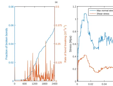
Figure 8. Temporal evolution of the fraction of broken bonds and

the rate of bond breaking (a); relationships between the fraction of broken bonds and the global normal and shear stress in simulations under uniaxial compression (reference model settings).

grain–grain forces are strong in regions subject to compres-sion and along fractures (bottom right in Fig. 11b), whereas bond-transmitted forces are strongest in regions under ten-sion.

8.2 Wave-induced sea ice fragmentation

In the second group of simulations, compact, undamaged sea ice is subject to flexural stresses generated by regular deep-water surface waves with a prescribed, spatially uni-form amplitudea, periodT and lengthL. All computations are performed until no bond breaking occurs. For the pur-pose of the basic verification of the model concept described in Sect. 6.3, simple one-dimensional (1-D) simulations are performed first (Sect. 8.2.1), in which a set ofN linearly ar-ranged identical grains bonded to their neighbors are subject to a prescribed propagating wave.

This 1-D setting is very close to a 2-D one in which a uni-directional wave propagates through a regular matrix of iden-tical grains, each bonded to its four neighbors. Because in this case the stresses acting on bonds oriented parallel to the wave crests, related to the Poisson effect, are close to zero, the model produces long parallel stripes with a breaking pat-tern exactly the same as that obtained with a 1-D model ver-sion. Therefore, in Sect. 8.2.2, devoted to 2-D simulations, only results obtained with an irregular arrangement of grains are analyzed, with a focus on the influence of this factor on the obtained floe sizes and shapes.

8.2.1 One-dimensional simulations

Let us consider a set ofN identical grains with radiusrand thicknessh, arranged regularly (with spacing 2r) along a line parallel to the wave propagation direction. In this case, in the

Time (s)

0 600 1200 1800 2400

0 0.02 0.04 0.06 0.08

(a)

Rate of bond breaking (10

-3s -1)

0 0.125 0.25 0.375 0.5

0 0.02 0.04 0.06

Stress (Mpa)

0 0.2 0.4 0.6 0.8 1 1.2

(b)

Max normal stress Shear stress

Figure 9. As in Fig. 8 but in simulation under shear strain.

absence of other forcing, the problem reduces to 2N+Nb

equations, whereNbdenotes the number of bonds:

dθi

dt =ωi, i=1, . . ., N, (35)

Ig

dωi

dt =Mvw,i+Mi,i+1−Mi,i−1, i=1, . . ., N, (36)

dMi,i+1

dt = −knIb(ωi−ωi+1), i=1, . . ., Nb. (37)

These equations follow directly from Eqs. (5), (7), and (17) with an assumption of the damping coefficientγd=1. Some

indices have been omitted for the sake of simplicity, and it is assumed thatIx1,i=Igfor all grains, andIx1,i,i+1=Iband

kn,i,i+1=knfor all bonds. If the initial floe is freely floating

on the sea surface, the outermost grains (i=1 and i=N) have only one neighbor,Nb=N−1 andM0,1=MN,N+1=

0. If one end of a floe is “frozen”, e.g., connected to the coast or the landfast ice that remains motionless, we setNb=N

and assumeωN+1=θN+1=0 andM0,1=0.

The wave forcing is calculated directly from Eq. (34), and the breaking criteria (Eqs. 19–22) reduce to a single one:

|Mi,i+1|hb/Ib> σt,max, (38)

where againhi,i+1=hbfor all bonds.

In the reference simulation summarized in Table 2, the ini-tial floe has length equal ton0L, wheren0=100 andLis the

wavelength, and with the selected grain radius of 3 m, there are roughly 26 grains per wavelength. Initially, no breaking is allowed (hence the infinite bond strength in Table 2) andn0is

varied to analyze the response of floes of various sizes to the wave forcing. Figures 12 and 13 show the range of variability of the grains’ tilt (separated into the rigid and flexural compo-nents) and the stress acting on bonds for three selected cases: small (n0=1 andn0=5) freely floating floes (Fig. 12a–d),

(15)

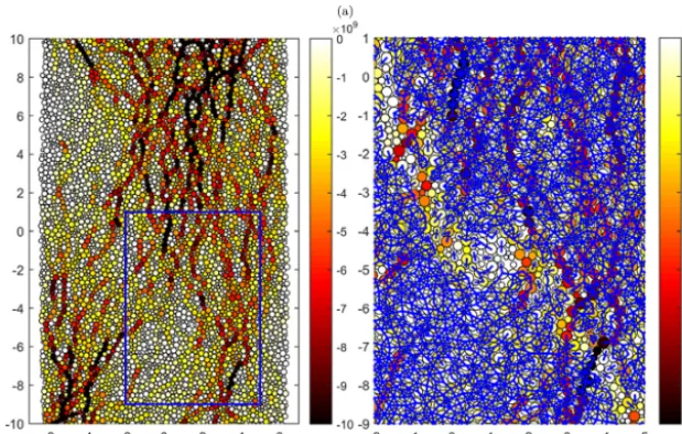
Figure 10. Instantaneous normal stress (color scale; in Pa) acting on individual grains in simulation under uniaxial compressive strain shortly

after terminal failure of the material (t=600 s; see Figs. 6 and 8). Panel (b) shows a fragment within the rectangle marked in (a), with bonds between grains illustrated with thick blue lines. Reference model settings.

Figure 11. Instantaneous shear stress (color scale; in Pa) acting on individual grains due to bond interactions (a) and pairwise interactions (b)

in simulation under shear strain att=2000 s (see Figs. 7 and 9). Reference model settings. Note different color scales in (a) and (b).

and connected to landfast ice (Fig. 13a, b). In all cases, three floe lengths,(n0−1₂)L,n0Land(n0+1₂)L, are considered,

because the motion of floes with lengths being an exact mul-tiple of the wavelength tends to be different from the mo-tion of similar floes that do not fulfill this criterion. Whereas in general, as expected, the amplitude of the rigid floe mo-tion increases with decreasing floe size, and for small floes (n0<10) exceeds the amplitude of the flexural motion by at

least an order of magnitude (compare continuous and dashed lines in Fig. 12a, c), the rigid motion remains negligible for floes with n0∈N, and their flexural response is dominated

by bending in the middle of the floe. Notably, the smallest floe considered, that of size 0.5L(green lines in Fig. 12a), follows the slope of the sea surface, which in the case

con-sidered reaches±1.15◦, almost exactly, even with a slight inertia-related “overshoot”. An analysis of periodograms of the grains’ tilts in the cases presented in Figs. 12 and 13 shows that for grains within large floes the power spectra have one dominating frequency – that of the external forcing – whereas additional peaks are present in spectra represent-ing grains within small floes, correspondrepresent-ing to the normal modes of the floes.

Understandably, if only one end of the floe is allowed to move freely, the above-mentioned influence of the exact ratio of the floe size to the wavelength is much less pronounced (Fig. 13a).

(16)

(a) (b)

Distance (x/L)

-0.6 -0.4 -0.2 0 0.2 0.4 0.6

Amplitude of rigid and flexural motion (degr)

-1.5 -1 -0.5 0 0.5 1 1.5

-0.6 -0.4 -0.2 0 0.2 0.4 0.6

Bond stress

σt

(10

5Pa

·

m

-1)

0 0.1 0.2 0.3 0.4 0.5 0.6

(c) (d)

-2.5 -2 -1.5 -1 -0.5 0 0.5 1 1.5 2 2.5

-0.15 -0.1 -0.05 0 0.05 0.1 0.15

-2.5 -2 -1.5 -1 -0.5 0 0.5 1 1.5 2 2.5

Bond stress

σt

(10

5Pa

·

m

-1)

0 0.05 0.1 0.15 0.2 0.25 0.3 0.35 0.4 0.45 0.5

(e) (f)

-50 -40 -30 -20 -10 0 10 20 30 40 50

-0.05 -0.04 -0.03 -0.02 -0.01 0 0.01 0.02 0.03 0.04 0.05

-50 -40 -30 -20 -10 0 10 20 30 40 50

Bond stress

σt

(10

5Pa

·

m

-1)

0 0.05 0.1 0.15 0.2 0.25 0.3 0.35 0.4 0.45 0.5

Distance (x/L)

Distance (x/L) Distance (x/L)

Figure 12. Results of 1-D simulations of sea ice response to waves (without breaking): tilt of the grains (a, c, e) and stress acting on bonds (b, d, f), for floe lengths equal to(n0−1₂)L(green),n0L(red) and(n0+1₂)L(blue);n0=1 in (a, b),n0=5 in (c, d), andn0=100 in (e, f).

In all cases, both ends of the floe could move freely (see text). The distance along the floes is measured relative to the floes’ centers. In (a,

c, e), continuous lines show the range of variability (i.e., the minimum and maximum values recorded during a simulation) of the flexural

components of the floe’s motion; analogously, the dashed lines show the range of variability of the rigid motion. In (b, d, f), the continuous and dashed lines show the maximum and the standard deviation of the stress, respectively. Note different ranges of the vertical axes in the panels. Note that in (a), the dashed and continuous red lines cannot be distinguished due to very small values.

it has a roughly exponential profile within the distance of 10–20 wavelengths from the free floe’s ends (Figs. 12e and 13a). This is extremely important from the point of view of stress acting on the ice (Figs. 12f and 13b) and,

(17)

(a) (b)

Distance (x/L)

-100 -90 -80 -70 -60 -50 -40 -30 -20 -10 0

-0.03 -0.02 -0.01 0 0.01 0.02 0.03

-100 -90 -80 -70 -60 -50 -40 -30 -20 -10 0

Bond stress

σt

(10

5Pa

·

m

-1)

0 0.05 0.1 0.15 0.2 0.25 0.3 0.35 0.4

Distance (x/L)

Figure 13. As in Fig. 12e, f, i.e., forn0=100, but for a floe with the right end “frozen” (see text). The distance along the floes is measured

relative to the floes’ right edges.

Table 2. Physical and numerical model parameters used in the

ref-erence simulations in Sect. 8.2.1.

Grains

Thickness h 1.0 m

Radius r 3.0 m

Bonds

Length coefficient λb 1.0 –

Radius coefficient λR 1.0 –

Thickness hm 0.8 m

Elastic modulus Eb 9.0×109 Pa

Tensile strength σt,max ∞ Pa

Waves

Amplitude a 0.5 m

Period T 10.0 s

No. of grains N 2602 –

Initial no. of bonds Nb N−1 –

the wave-induced stresses exceed this value close to the floe edge, but not in its inner parts. In this case, breaking starts at the floe boundary, gradually progresses deeper into the ice, and continues until no floes larger than 0.5Lremain (inset in Fig. 14a). The pattern of dots in Fig. 14 shows that break-ing events are clustered and tend to occur in series spannbreak-ing a few wavelengths and a small fraction of the wave period. Indeed, almost 40 % of breaking events occur within the dis-tance of one wavelength from the previous one, and the his-togram of distances between subsequent breaking events has a clear maximum at∼0.25L(not shown). The final pattern of floe sizes is not perfectly regular (Fig. 14b), but there is

(a)

Distance (x/L)

-100 -90 -80 -70 -60 -50 -40 -30 -20

Time (t T )

2 3 4 5 6 7 8

Floe size (l L )

0 0.2 0.4 0.6

0 100 200

(b)

-100 -98 -96 -94 -92 -90 -88 -86 -84 -82 -80

–1

Distance (x/L)

Figure 14. Wave-induced breaking of an ice floe with initial size

100L, “frozen” at its right end (x=0). In the main panel in (a), individual breaking events are shown with dots in function of their position and time. The inset in (a) shows the histogram of the floe sizes (l/L) after breaking. In (b), a fragment of the initial floe, 20L

long, is shown, with breaking positions marked with vertical lines.

(18)

Two aspects of these results are worth stressing. First, this breaking pattern, progressing from the ice edge towards in-ner regions, has been obtained with a spatially constant wave amplitude. In a more realistic configuration, with wave am-plitude decreasing with the distance from the ice edge due to attenuation, this effect would be even stronger. Second, with a constant wave amplitude, progressive breaking is possible only if the wave-induced stress acting on the ice far from its edge remains smaller than its strength. In real-world situa-tions, such “tuning” of the wave steepness to the ice strength is presumably rare in stationary settings, but can be expected to occur frequently during periods of wave amplitude in-creasing in time, e.g., when the onshore wind strengthens or when swell from distant locations arrives at the ice edge with gradually increasing amplitude. Thus, breaking similar to that shown in Fig. 14 may be more frequent than the over-simplified model setting used here suggests. On the other hand, obviously, the great majority of combinations of the model parameters produce either very strong, almost instan-taneous fragmentation of the whole initial floe (with the ma-jority of bonds destroyed and a clearly defined maximum floe size) or almost no fragmentation (with only a very small frac-tion of bonds broken).

8.2.2 Two-dimensional simulations

As already mentioned in the introduction to this section, a 2-D model initialized with a regular, square matrix of identical grains produces floes in the form of long stripes parallel to the wave crests. However, in order for the model to be ap-plicable to more general conditions, e.g., with waves coming from different directions, it is desirable that the model pro-duces realistic results (in terms of both floe sizes and shapes) when it is initialized with randomly distributed grains of dif-ferent sizes, and thus contains bonds with a range of spatial orientations not aligned with the wave direction.

As can be expected, most aspects of the behavior of the 2-D model are fully analogous to those of the 1-D model. In particular, the dependence of the amplitude of the flex-ural and rigid motions of the floes on their size, described in the previous section, is very similar in 1-D and 2-D. As previously, the model has been run for a reference run (Ta-ble 3) and for a set of configurations with one selected param-eter varied. Obviously – as in the 1-D case – most combina-tions of the coefficients produce either almost no breaking or very intense breaking (like that shown in Fig. 15b). However, within a narrow range of the model parameters between these two “regimes”, breaking results in floes with rather unrealis-tic shapes, with “branches” of connected grains stretching in different directions (some of these features can be seen in Fig. 15a) or even floes with “holes” in the middle, filled with loose grains or smaller floes. This tendency for “branching” floes to survive breaking is related to another rather pecu-liar aspect of these configurations: a wide range of sizes of the floes. For example, as shown in Fig. 16, for wave

pe-Table 3. Physical and numerical model parameters used in the

ref-erence simulations in Sect. 8.2.2.

Grains

Thickness h 1.5 m

Minimum radius r_min 12.5 m

Maximum radius rmax 37.5 m

Elastic modulus E 6.0×109 Pa

Poisson’s ratio ν 0.33 –

Static yield criterion µ 0.7 –

Bonds

Length coefficient λ_b 0.4 –

Radius coefficient λR 1.0 –

Mean thickness hm 0.5 m

Width of thick. distr. δh 0.0 m

Ratio of normal to shear stiffness λns 2.0 –

Elastic modulus E_b 9.0×109 Pa

Compressive strength σc,max 5.0×105 Pa

Tensile strength σt,max 5.0×104 Pa

Shear strength τmax 5.0×104 Pa

Waves

Amplitude a 1.5 m

Period T 25.0 s

No. of grains N 30 000 –

Initial no. of bonds N_b 73 421 –

riodT =25 s (i.e., the reference run, illustrated in Fig. 15a) the floe sizes span at least 3 orders of magnitude. The re-sults are very different for both longer and shorter waves. With wave periods of less than 23 s, hardly any floes contain more than 10 grains (Figs. 16 and 15b); with wave periods higher than 26 s, a few largest floes contain more than 90 % of all grains in the system; i.e., most of the ice remains in-tact. Varying other model parameters produces similar model behavior; see Figs. S5 and S7 for examples showing the ef-fects of changing the mean bond thicknesshmand the bond

elastic modulusEb, respectively. (Notably, increasing spatial

variability of the bonds’ thickness, and thus their stiffness, has almost no influence on the resulting floe-size distribu-tion; see Fig. S6.)

(19)

Figure 15. Fragments of the model domain at the end of the reference simulation, withT =25 s (a; wavelengthL=976 m), and a simulation withT =23 s (b; wavelengthL=826 m), showing the pattern of floes. The wave propagation direction is from top to bottom. Note that the whole area of both panels is covered with ice; i.e., the large white spaces are large floes, not open water.

Figure 16. Rank-order statistics of floe sizes (a: number of grains in a floe; b: floe surface area) obtained in simulations with different wave

periodsT. The dashed line in (b) marks the area of the largest individual grain in the ensemble. Results of the reference run are shown with crosses.

non-convex floes decreases with increasing shear stiffness and decreasing shear strength of bonds (relative to their nor-mal stiffness and compressive strength, respectively), but it remains to be investigated whether adjusting these parame-ters accordingly does not produce any other negative effects. In any case, the general conclusion is that the orientations of bonds in the model do determine the resulting geometry of the floes. In particular, although the floes tend to be elongated in the direction of the wave crests (Fig. 15), it is not possible to obtain long stripes even with perfectly unidirectional wave forcing.

9 Discussion and further perspectives

The modeling results presented in this paper have been lim-ited to very simple configurations, with the goal of testing the basic model features and analyzing the influence of the model parameters on its behavior. Further work is necessary