doi:10.5194/gmd-8-1493-2015
© Author(s) 2015. CC Attribution 3.0 License.
An improved representation of physical permafrost dynamics in the
JULES land-surface model
S. Chadburn1, E. Burke2, R. Essery3, J. Boike4, M. Langer4,5, M. Heikenfeld4,6, P. Cox1, and P. Friedlingstein1 1Earth System Sciences, Laver Building, University of Exeter, North Park Road, Exeter EX4 4QE, UK
2Met Office Hadley Centre, Fitzroy Road, Exeter EX1 3PB, UK
3Grant Institute, The King’s Buildings, James Hutton Road, Edinburgh EH9 3FE, UK
4Alfred Wegener Institute, Helmholtz Center for Polar and Marine Research (AWI), 14473 Potsdam, Germany
5Laboratoire de Glaciologie et Géophysique de l’Environnement (LGGE) BP 96 38402 St Martin d’Hères CEDEX, France 6Atmospheric, Oceanic and Planetary Physics, Department of Physics, University of Oxford,
Parks Road, Oxford OX1 3PU, UK
Correspondence to: S. Chadburn ([email protected])
Received: 19 December 2014 – Published in Geosci. Model Dev. Discuss.: 30 January 2015 Revised: 28 April 2015 – Accepted: 30 April 2015 – Published: 21 May 2015
Abstract. It is important to correctly simulate permafrost in global climate models, since the stored carbon represents the source of a potentially important climate feedback. This car-bon feedback depends on the physical state of the permafrost. We have therefore included improved physical permafrost processes in JULES (Joint UK Land Environment Simula-tor), which is the land-surface scheme used in the Hadley Centre climate models.
The thermal and hydraulic properties of the soil were mod-ified to account for the presence of organic matter, and the in-sulating effects of a surface layer of moss were added, allow-ing for fractional moss cover. These processes are particu-larly relevant in permafrost zones. We also simulate a higher-resolution soil column and deeper soil, and include an ad-ditional thermal column at the base of the soil to represent bedrock. In addition, the snow scheme was improved to al-low it to run with arbitrarily thin layers.
Point-site simulations at Samoylov Island, Siberia, show that the model is now able to simulate soil temperatures and thaw depth much closer to the observations. The root mean square error for the near-surface soil temperatures reduces by approximately 30 %, and the active layer thickness is re-duced from being over 1 m too deep to within 0.1 m of the observed active layer thickness. All of the model improve-ments contribute to improving the simulations, with organic matter having the single greatest impact. A new method is
used to estimate active layer depth more accurately using the fraction of unfrozen water.
Soil hydrology and snow are investigated further by hold-ing the soil moisture fixed and adjusthold-ing the parameters to make the soil moisture and snow density match better with observations. The root mean square error in near-surface soil temperatures is reduced by a further 20 % as a result.
1 Introduction
The northern high latitudes (NHLs) are an important region in terms of the changing global climate. Both observations and future projections of warming are amplified in this re-gion (Overland et al., 2004; Bekryaev et al., 2010; Stocker et al., 2013). At the land-surface scale, significant thawing of permafrost has already been observed in many areas (Camill, 2005; Romanovsky et al., 2010, 2013).
make future climate projections and inform emissions targets (Stocker et al., 2013).
In order to include permafrost carbon feedbacks in land-surface models, the first requirement is that the physics is simulated correctly. This includes thaw depth and rate of thaw, hydrological processes and soil temperature dynamics, which all affect soil carbon stocks and decomposition rate (Gouttevin et al., 2012b; Exbrayat et al., 2013).
While permafrost-specific models have made progress to-wards correctly simulating permafrost dynamics (Risebor-ough et al., 2008; Jafarov et al., 2012; Westermann et al., 2015), in global land-surface models the Arctic has often been neglected, leading to the large discrepancies between models and reality seen in Koven et al. (2012). One reason that the NHLs are poorly represented in global models is the difficulty of obtaining observations with which to drive and evaluate the models. Harsh conditions in the Arctic mean that much of the land area is difficult to access, and detailed sim-ulations are only possible on small scales. However, the use of small-scale simulations where observations are available can help to improve the large-scale dynamics. Several global land-surface models have already improved their representa-tion of permafrost physics (Beringer et al., 2001; Lawrence and Slater, 2008; Gouttevin et al., 2012a; Ekici et al., 2014a). In this paper we add new permafrost-relevant processes into JULES (Joint UK Land Environment Simulator), which is the land-surface scheme in the Hadley Centre climate mod-els and will be used in the first UK Earth system model (Best et al., 2011; Clark et al., 2011), improving on the past im-plementation of these processes (Christensen and Cox, 1995; Cox et al., 1999). We evaluate the model at a site level, where it is reasonable to compare the model directly with observa-tional data, and a large quantity of data is available. Being able to simulate realistically at a site level shows that the physics of the model is correct, which is a prerequisite for trusting large-scale simulations. These developments are in-cluded in large-scale simulations in Chadburn et al. (2015).
JULES already includes some of the processes that are im-portant for permafrost: the effects of soil freezing and thaw-ing on the energy budget and, more recently, a multilayer snow scheme, which significantly improves model perfor-mance (Burke et al., 2013). However, systematic differences between JULES simulations and reality have been identified. When compared with observations of active layer thickness (ALT) (thickness of seasonally frozen layer), the simulated active layer in JULES is consistently too deep. This is seen, for example, in Dankers et al. (2011), where the simulated active layer was compared with observations from over 100 sites in the CALM (Circumpolar Active Layer Monitoring Network) active layer monitoring programme (Brown et al., 2000). This bias in ALT indicates that the soil may warm too quickly in summer, which would lead to an amplification of the annual cycle of soil temperatures. This amplification is indeed observed in JULES (Burke et al., 2013). This sug-gests that the model undergoes an accelerated soil warming
in summer, meaning either that too much heat enters the soil or too much of that heat accumulates near the surface.
There are two controls on the amount of heat entering and leaving the soil: the land-cover above the soil and the thermal properties of the soil itself. In particular, soil organic matter and the moss layer that is often present in the low Arctic can greatly influence the ALT and summer soil temperatures (Dyrness, 1982). This is because moss and organic matter have insulating properties and can also hold more water than mineral soils. The importance of accounting for organic mat-ter in land-surface models has been discussed in e.g. Rinke et al. (2008), Lawrence et al. (2008), and Koven et al. (2009). Snow also insulates the soil in winter and has a very large ef-fect on the soil temperatures and permafrost dynamics (West-ermann et al., 2013; Langer et al., 2013; Ekici et al., 2014b). Thus, in this model development work, we consider imple-menting the physical effects of moss and organic matter, and further improving the snow scheme in JULES.
An accumulation of heat near the surface in the model can be related to the heat sink of the deeper part of the soil: if the model does not simulate a deep soil column this heat sink is missing. Several studies have shown that a shallow soil col-umn does not give realistic temperature dynamics (Stevens et al., 2007; Alexeev et al., 2007). Finally, the resolution of the soil column affects the numerical accuracy of the sim-ulation and also the precision to which the ALT can be re-solved. The default configuration for JULES represents only the top 3 m of soil with four layers. Therefore, in this work the depth and resolution of the soil column is increased, in-cluding a thermal “bedrock” column at the base.
The impact of soil hydrology is also considered, showing that if the soil moisture were simulated correctly the simula-tions of soil temperature could be further improved. Soil tem-peratures are affected by the water content of the soil not only through its thermal properties but also via the latent heat of freezing, which slows down the rate of temperature change.
Simulations are performed of the Samoylov Island site in Siberia, adding each model development in turn. This shows the impact of the new processes and significant improve-ments to model performance and the representation of per-mafrost in JULES. Areas for future development are also clearly identified.
2 Methods
2.1 Model description (standard version)
and is available at http://www.jchmr.org/jules. The work dis-cussed here builds upon JULES version 3.4.1.
JULES simulates the physical, biophysical and biochemi-cal processes that control the exchange of radiation, heat, wa-ter and carbon between the land surface and the atmosphere. It can be applied at a point or over a grid and requires a con-tinuous time series of atmospheric forcing data at a frequency of 3 h or greater. Each grid box can contain several different land covers or “tiles”, including a number of different plant functional types (PFTs) as well as non-vegetated tiles (urban, water, ice and bare soil). Each tile has its own surface energy balance, but the soil underneath is treated as a single column and receives aggregated fluxes from the surface tiles.
JULES uses a multilayer snow scheme (described in Best et al., 2011) in which the number of snow layers varies ac-cording to the depth of the snowpack. Each snow layer has a prognostic temperature, density, grain size and water con-tent. In the old, zero-layer snow scheme, the insulation from snow was incorporated into the top layer of the soil. This scheme is currently still used when the snow depth is below 10 cm.
The subsurface temperatures are modelled via a discreti-sation of both heat diffusion and heat advection by moisture fluxes. The soil thermal characteristics depend on the mois-ture content, as does the latent heat of freezing and thawing. A zero-heat-flux condition is applied at the lower boundary. The soil hydrology is based on a finite difference approxima-tion of Richards’ equaapproxima-tion (Richards, 1931), with the same vertical discretisation as the soil thermodynamics (Cox et al., 1999). JULES uses the Brooks and Corey (1964) relations to describe the soil water retention curve and calculate hy-draulic conductivity and soil water suction. Soil hyhy-draulic and thermal parameters are input to the model via an ancil-lary file. The default vertical discretisation is a 3 m column modelled as four layers, with thicknesses of 0.1, 0.25, 0.65 and 2 m.
The land-surface hydrology scheme (LSH) simulates a deep water store at the base of the soil column and allows for subsurface flow from this layer and any other layers be-low the water table. Topographic index data is used to gener-ate the wetland fraction and saturation excess runoff (Gedney and Cox, 2003).
JULES also includes a dynamic vegetation model, TRIF-FID, which simulates vegetation competition to determine the grid-box fraction assigned to each PFT (Cox, 2001). JULES may also be run with TRIFFID switched off and a fixed vegetation fraction, which was the case for the simu-lations in this paper, where the focus is on the physical pro-cesses.
2.2 Permafrost model developments
Model developments include the thermal effects of a surface moss layer, the thermal and hydrological effects of soil or-ganic matter, a thermal “bedrock” column beneath the
ordi-nary soil, and an improvement of the multilayer snow scheme to allow for arbitrarily thin layers. The resolution and depth of the soil column is also increased. These improvements are described in detail in the following subsections.
2.2.1 Moss
The characteristics of moss will vary between different species and ecosystems, but all mosses will insulate the soil. Therefore, the thermal conductivity of the soil was modified to represent this insulating layer. Its purpose in these simu-lations is to give a somewhat generic representation of the thin layer of moss-rich vegetation which is abundant in the Arctic. Although any vegetation layer in JULES has an insu-lating effect thanks to the canopy heat capacity (Best et al., 2011), this new type is necessary because the current PFT’s are not appropriate for Arctic tundra.
The thermal conductivity of moss depends on its water content. For simplicity we assume that the moss layer co-incides with the top layer of the soil, and thus has the same hydraulic suction. The water content is then calculated from the suction using the Brooks and Corey (1964) equation,
θmoss θsat,moss
=
ψ
ψsat,moss −bmoss
, (1)
whereθ is the volumetric water content, ψ is the soil wa-ter suction, b is the exponent and the subscript sat refers to the values at saturation. The following hydraulic param-eters were used for moss (Beringer et al., 2001):bmoss=1, ψsat,moss=0.12 m,θsat,moss=0.9.
The dependence of moss thermal conductivity on wa-ter content was measured by Soudzilovskaia et al. (2013). We choose the representative values for the saturated conductivity of 0.5 Wm−1K−1 and for dry conductivity 0.06 Wm−1K−1, and linearly interpolate between the two depending on the moisture content (Eq. 1). These are also consistent with the values given for organic soils in Williams and Smith (1991).
The user can choose the thickness of the moss layer; the default value is 5 cm. The thermal conductivity of the top 5 cm of soil is then modified according to the parameters above. This is applied to a fraction of the grid-box depending on a variable representing the percentage cover of moss. 2.2.2 Organic soils
Organic soils were previously considered in JULES by Dankers et al. (2011), who concluded that their effects were small. In this paper, however, we use an improved implemen-tation of their impact.
avail-able in kilograms per cubic metre, which were converted to a volumetric fraction using literature values for the density (800 kg m−3) and porosity (Dankers et al., 2011, Table 2) of organic matter.
For some of the soil properties, the organic fraction was used to provide a linear weighting of organic and mineral characteristics (Appendix A, Eqs. A1, A4, A7), as in Dankers et al. (2011) and other similar work. However, the saturated hydraulic conductivity, dry thermal conductivity and satu-rated soil water suction were calculated using a more ap-propriate non-linear aggregation (Appendix A, Eqs. A2, A3, A8). As a result, the organic components of the dry ther-mal conductivity and saturated water suction have a larger effect than if they were calculated via a linear weighted aver-age. See Appendix A for details. New soil properties, which include the effects of organic matter, may now be input to JULES via an updated soil ancillary file.
The current parameterisation of saturated thermal conduc-tivity in JULES (Dharssi et al., 2009) restricts the values to those appropriate for mineral soils. Organic soils have a much lower saturated thermal conductivity, so it was neces-sary to modify the Dharssi parameterisation to take account of this.
The thermal conductivity of dry soil (λdry) is input to JULES via the ancillaries, and the saturated thermal conduc-tivity is calculated in the model, depending on the fraction of the soil moisture that is currently frozen. The actual value of thermal conductivity is then calculated by interpolating be-tween the dry and saturated conductivities depending on the water content. The literature values used in JULES for the dry thermal conductivity are 0.25 Wm−1K−1 for clay soils and 0.3 Wm−1K−1 for sandy soils, and saturated conduc-tivity of 1.58 and 2.2 Wm−1K−1, respectively (for unfrozen soils) (Williams and Smith, 1991, Table 4.1).
For organic soils, the dry conductivity is approxi-mately 0.06 Wm−1K−1 and the saturated conductivity 0.5 Wm−1K−1(Williams and Smith, 1991). However, using Dharssi’s method the minimum value for saturated conduc-tivity is 1.58 Wm−1K−1. It was therefore necessary to im-plement a parameterisation of saturated thermal conductivity that extends to the appropriate values, for which a smooth curve was fitted to the data (Appendix A, Eq. A11). The two curves are shown in Fig. 1. The conductivities for mineral soils will be slightly different in the new formulation, but this difference will be small and well within the uncertainty of the literature values.
Note that the same thermal conductivity values are used for both moss and organic soil. This is consistent with the fact that, for example in peat soils, the layer of living moss can be almost indistinguishable from the surface organic layer. One good reason for treating them separately, however, is that moss can also grow in places without a pronounced or-ganic layer.
Figure 1. New method of calculating saturated thermal
conductiv-ity (λsat0) from dry thermal conductivity (λdry), compared with the standard method. See Appendix A, Eq. (A10) for the Dharssi pa-rameterisation and Appendix A, Eq. (A11) for the new method, which is modified to include organic soils.
2.2.3 Increased soil resolution and depth
The hydrologically active soil column is run in three dif-ferent configurations, beginning with the standard four-layer configuration, with layer thicknesses of 0.1, 0.25, 0.65 and 2.0 m. The second configuration increases the soil resolution without increasing the depth, having 14 layers in 3 m of soil. The layer thicknesses start at 0.05 m and increase with depth according to the function dzn=0.05n0.75. Finally, the
high-resolution column is extended to 10 m with a total of 28 lay-ers, following the same function for dzn.
In this last case, soil column depth is increased even fur-ther by adding an extra column to the base of the hydro-logically active column, to represent bedrock. This bedrock column adds another 50 m, bringing the total soil column to 60 m. See Sect. 2.2.4 for details.
2.2.4 Bedrock thermal dynamics
A bedrock column was added to JULES, starting at the base of the hydrologically active soil column. We assume that the heat transfer in this deep column is not influenced by hydro-logical processes. This allows for the representation of a deep soil column without a large computational load. Heat transfer is simulated by thermal diffusion:
Cdeep ∂Ts,deep
∂t =λdeep
∂2Ts,deep
∂z2 , (2)
Cdeep
Ts,deep(i+1, n)−Ts,deep(i, n)
δt =
λdeep
Ts,deep(i, n+1)−2Ts,deep(i, n)+Ts,deep(i, n−1)
dz2deep , (3)
where i indexes the timesteps and n indexes the vertical layers. This uses a constant heat capacity, Cdeep, and ther-mal conductivity,λdeep, which may be set by the user. The default values are Cdeep=2.1×10⁶JK−1m−3 and λdeep= 8.6 Wm−1K−1(the properties of the soil solids in sand from Beringer et al. (2001), and very close to the values for quartz in Williams and Smith, 1991). By default, the vertical layer thickness is dzdeep=0.5 m, with 100 layers, resulting in an extra 50 m soil column, but the user can also set these val-ues. In most models the deep soil is not so finely resolved – in fact it is often represented as a single thick layer, but since the heat diffusion is so computationally light, there is no reason not to resolve the dynamics more accurately.
In the hydrologically active soil column an implicit solu-tion is used for the temperature increments, but for bedrock the explicit solution is sufficient since temperature changes are slow and there are no freeze–thaw processes to consider. The heat flux across the boundary with the base of the hydro-logically active soil column is
heat flux=λbase
(Ts(i, N )−Ts,deep(i,1)) 0.5(dzdeep+dz(N ))
, (4)
where the thermal conductivity,λbase, is an interpolation be-tween the bottom layer of the hydrological column and the top layer of the bedrock column. Here N is the number of soil hydrological layers, which interface with the bedrock column. The heat flux at the base of the bedrock column is set to zero by default, but could be set to the geothermal heat flux in future versions.
2.2.5 Improved snow scheme
The original release of JULES included the same simple snow model as in the MOSES land-surface scheme (Cox et al., 1999) and the HadCM3 (Hadley Centre Coupled Model, version 3) climate model. In this model version, snow on the ground was represented by a modification of the prop-erties of the surface layer in the soil model. The multilayer snow model described by Best et al. (2011) was introduced as an option in JULES version 2.1 and was found to give signif-icantly improved predictions of soil temperatures under deep snow (Burke et al., 2013), but the old snow model was re-tained for shallow snow of less than 10 cm depth to avoid nu-merical instabilities. For this study, a modification has been implemented that allows shallow snow to be represented by a distinct model layer. This is done by calculating the heat flux into the snow or soil surface according to the temper-ature gradient between the surface and a fixed depth below
Samoylov
Figure 2. Map showing location of Samoylov Island and Northern
Hemisphere permafrost distribution (Brown et al., 1998).
the surface. The snow layer temperature is stepped forward in time using the backward Euler method, which remains sta-ble for an infinitesimal layer thickness.
2.3 Samoylov Island site information
Point-scale simulations were carried out using data from the Samoylov Island field site in the Lena River delta, Siberia. Figure 2 shows the location of Samoylov Island in the context of the whole Arctic permafrost region. There is a large quan-tity of data available from this site, making it a good site for detailed process evaluation (e.g. Yi et al., 2014). The land-scape is formed of ice-wedge polygonal tundra with ponds and thermokarst lakes. There is an abundance of mosses and organic soil, so including the model developments described above has a notable impact on the JULES simulations. A typ-ical soil profile is shown in Fig. 3b, highlighting the moss and organic layers. Figure 3a shows an aerial view of the moni-toring site, including the meteorological station, soil temper-ature monitoring and active layer monitoring grid (only poly-gon centre points are highlighted as these data are used for evaluation). A detailed description of the site may be found in Boike et al. (2013).
2.3.1 Forcing data
Moss cover
Peat & fine sand (active layer)
Silt & fine sand (active layer)
Silt & fine sand (permafrost)
Soil temperature monitoring site Active layer
monitoring field
0 2 10 m
N Climate station
(a) (b)
Figure 3. Images from the Samoylov Island site. (a) Aerial view
showing monitoring stations. (b) Typical soil profile showing moss layer, organic layer and mineral soil.
grid cell containing the site. For the period 1901–1979, water and global change forcing data (WFD) were used (Weedon et al., 2010, 2011). This is a meteorological forcing data set based on ERA-40 reanalysis (ECMWF, 2006), with correc-tions generated from Climate Research Unit (CRU) (Mitchell and Jones, 2005) and Global Precipitation Climatology Cen-tre (GPCC) data (http://gpcc.dwd.de). Data is provided at half-degree resolution for the whole globe at 3-hourly time resolution from 1902 to 2001, with years prior to 1958 based on random years from ERA-40 but corrected with observa-tions from the relevant time period. For the period 1979– 2010, WATCH Forcing Data Era-Interim (WFDEI) was used (Weedon, 2013). This is produced using the same techniques as the WFD but is instead based on the ERA-Interim reanal-ysis data (ECMWF, 2009) and covers the period 1979–2012. For the time periods where observed data were available from Samoylov, correction factors were generated by calculating monthly biases relative to the WFDEI data. These corrections were then applied to the time series from 1979 to 2010 of the WFDEI data. The WFD before 1979 was then corrected to match this data and the two data sets were joined at 1979 to provide gap-free 3-hourly forcing from 1901 to 2010.
Meteorological station observations were used for all vari-ables except snowfall, which was estimated from the ob-served snow depth by treating increases in snow depth as snowfall events with an assumed snow density of 180 kg m−3. Snow depth observations are available daily from 2002 to 2013, although with some missing years. These reconstructions were then used to provide correction factors to WFDEI and WFD. This leads to a more realistic snow depth in the model than using direct precipitation measure-ments, due to wind effects and the difficulty of accurately measuring snowfall.
2.3.2 Soil and land-cover characteristics
The land characteristics were chosen to represent a depressed polygon centre, and the evaluation data (soil temperatures, moisture, etc.) were also taken from polygon centre measure-ments (see Fig. 3a).
The mineral soil is a sandy loam and was assumed to have 50 % silt, 45 % sand, 5 % clay, which is consistent with the information in Boike et al. (2013). The soil prop-erties were calculated using the Cosby et al. (1984) relations. Site-specific organic carbon quantities are given in Zubrzy-cki et al. (2013), but there is significant heterogeneity, with values for polygon centres ranging between 3 and 85 kg m−3. The mean values of 25 kg m−3of organic carbon above 30 cm and 35 kg m−3 from 30 cm to 1 m were used, giving a vol-umetric fraction forg between 0.4 and 0.6. Following the model set-up used in Langer et al. (2013), organic carbon below 1 m was taken as zero. The transition between car-bon quantities above and below 30 cm was smoothed into a curve. Organic properties were then combined with the mineral properties as in Sect. 2.2.2.
To verify this parameterisation of organic soil properties in JULES, we compare the resulting thermal properties with those in Langer et al. (2011a, b). We compare saturated values in JULES with values for saturated peat. In JULES the thermal conductivity is consistent with the Langer val-ues, lying between 0.7 and 0.9 Wm−1K−1when thawed and between 1.9 and 2.1 Wm−1K−1 when frozen. The values from Langer et al. (2011a, b) are 0.72±0.08 (thawed) and 1.92±0.19 Wm−1K−1(frozen). The heat capacity in JULES is 3.5–3.8 (thawed) and 2.2–2.3 MJ m−3K−1(frozen), which is again close to the Langer values of 3.8±0.2 (thawed) and 2.0±0.05 MJ m−3K−1(frozen); although the heat capacity when frozen is a little too high in JULES, this is a reasonable level of consistency given the high spatial variability in soil properties.
The vegetation at Samoylov is composed predominantly of mosses, along with grasses and small shrubs with about 10 % coverage. The land cover in JULES was taken as 10 % grass with a height of 10 cm. Moss cover was set to 90 % (or 90 % bare soil in simulations without moss).
For simulations with higher-resolution and deeper soil, the set-up is described in Sect. 2.2.3. The new bedrock routine was also used (Sect. 2.2.4), adding a further 50 m heat sink to the base of the soil. Samoylov Island sits above a deep river deposit, so the deep soil is composed of silt deposits. The estimated parameters for the deep soil are approximately Cdeep=2.1 MJ m−3K−1andλdeep=2 Wm−1K−1, so these values were used for the bedrock column in JULES (Boike et al., 2013).
Figure 4. Thaw depth for thawing period in 2006. JULES
simula-tion orgmossDS compared with observasimula-tions, showing the differ-ence between two methods of calculating thaw depth. The tempera-ture method (red line) is limited by the resolution of the soil layers. Observations are means with error bars showing the full range.
still too low, since the observed density for a polygon centre is around 230 kg m−3. However, 190 kg m−3 is close to the spatial average given in Boike et al. (2013) and this is also ap-proximately consistent with the assumed value of 180 kg m−3 used to create the driving data. This is considered further in Sect. 3.2.
The LSH scheme was also switched on (see Sect. 2.1). This scheme adds a deep water store at the base of the soil and thus improves the water-holding capacity of the soil. 2.3.3 Simulation set-up
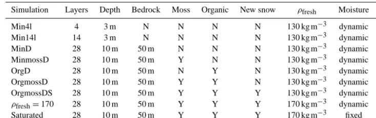
Simulations were performed first for the standard version of JULES using just mineral soil (min4l). The developments of increased soil discretisation (min14l), deeper soil (minD), or-ganic soil properties (orgD), moss insulation (orgmossD) and the improved snow scheme (orgmossDS) were then system-atically introduced (see Table 1), with the final simulation containing all of the model improvements (orgmossDS). The simulations labelledρfresh=170 and Saturated in Table 1 are discussed in Sect. 3.2.
The simulations were spun-up for 200 years using the first 10 years of driving data (starting at 2 January 1901), by which point the soil temperatures and water contents were stable. They were then run from 1901 until the end of 2010. 2.4 Calculating active layer thickness (ALT)
Commonly used methods of calculating ALT in land-surface models make use of the soil temperatures, either by taking the depth of the deepest layer that is above 0◦C or an
inter-polation of soil temperatures to find the depth of 0◦C; see for example Koven et al. (2012) and Lawrence et al. (2012). However, this method is limited by the vertical discretisa-tion. In JULES, when a given layer is freezing or thawing, the temperature of the layer remains very close to 0◦C for the duration of freeze–thaw, with the consequence that any interpolation puts the thaw depth very close to the centre of
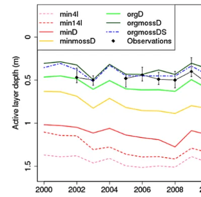
Figure 5. Simulated active layer depth at Samoylov since 2000.
Ob-servations show the mean thaw depth from polygon centre active-layer monitoring points (see Fig. 3), with error bars indicating the range of measured values. Simulations begin with the standard four-layer JULES (min4l), and improvements are systematically added: higher-resolution soil (min14l), deeper soil (minD), moss cover (minmossD), organic soils (orgD, orgmossD), and the improved snow scheme (orgmossDS).
the layer. However, more information may be extracted from JULES by outputting the frozen and unfrozen water contents in the layer. In this paper, the ALT is calculated by taking the unfrozen water fraction in the deepest layer that has begun to thaw and assuming that this same fraction of the soil layer has thawed. This is represented by the following equation:
ALT= X
i=1,n
dzi+
θu,n+1 θu,n+1+θf,n+1
dzn+1, (5)
whereθf andθu are frozen and unfrozen water content as a fraction of saturation, andnis the deepest layer that has completely thawed (θf,n=0). This gives significantly more
Table 1. List of JULES simulations carried out.ρfreshis the density of fresh snow.
Simulation Layers Depth Bedrock Moss Organic New snow ρfresh Moisture
Min4l 4 3 m N N N N 130 kg m−3 dynamic
Min14l 14 3 m N N N N 130 kg m−3 dynamic
MinD 28 10 m 50 m N N N 130 kg m−3 dynamic
MinmossD 28 10 m 50 m Y N N 130 kg m−3 dynamic
OrgD 28 10 m 50 m N Y N 130 kg m−3 dynamic
OrgmossD 28 10 m 50 m Y Y N 130 kg m−3 dynamic
OrgmossDS 28 10 m 50 m Y Y Y 130 kg m−3 dynamic
ρfresh=170 28 10 m 50 m Y Y Y 170 kg m−3 dynamic
Saturated 28 10 m 50 m Y Y Y 170 kg m−3 fixed
3 Results and discussion 3.1 Soil temperatures and ALT
Figure 5 shows the simulated ALT at Samoylov over the 11-year period 2000–2010. It is clear that many of the new pro-cesses in the model reduce the ALT, with the final simulation including deep soil, moss, organic properties and the new snow scheme (orgmossDS) bringing the simulated ALT very close to the observations. In orgmossDS the ALT falls within the range of observations for every year where measurements are available. A significant bias of over 1 m for the standard JULES set-up (min4l) has been removed by including these model developments.
Comparing the first two simulations, min4l and min14l, the mean ALT is reduced by 0.2 m when soil resolution is increased. The base layer in min4l is 2 m thick, and the thaw depth consistently reaches almost to the centre of this layer, although in some years earlier in the simulation (not shown) the thaw reaches only the third model layer and thus the ALT changes by approximately 0.5 m in 1 year, which is unrealis-tic behaviour.
A comparison of shallow and deep simulations, both with high resolution (min14l and minD in Fig. 5) demonstrates that there is a small but significant reduction in bias when the depth of the soil column is increased to 10 m and bedrock is added. In this case the mean ALT is reduced by 0.13 m.
The addition of the organic soil parameterisation has the single biggest impact on the ALT in these simulations. The mean ALT in minD is 1.03 m, and in orgD it is 0.49 m, a reduction of over half a metre. Moss on its own also has a large impact, reducing the mean ALT by 0.35 m from minD to minmossD. However, the effects are non-linear: compar-ing orgD and orgmossD, the mean ALT is reduced by only 0.17 m by the addition of moss.
The ALT depends on the maximum soil temperatures in summer, but it is important to simulate the correct soil tem-peratures for the whole year and the whole soil column. Ta-ble 2 shows some key performance metrics for the soil tem-peratures at different depths, most of which are significantly improved in the final simulation (orgmossDS). This shows
that although the changes to the snow scheme have very lit-tle effect on the ALT, they reduce the root mean square error (RMSE) in upper soil temperatures from 4.1 to 3.4◦C, which is a significant improvement.
The simulated active layer temperatures in the mineral soil simulations (min4l, min14l and minD), shown in Table 2, are too warm (≈2◦C) and the annual cycle is much too large. This is consistent with the large-scale biases in JULES dis-cussed in Sect. 1. The addition of organic soils and moss re-duces the mean active layer temperature and annual cycle to more realistic values. The changes to the snow scheme then increase the active layer temperature by 1.2◦C, but the
tem-perature bias is still less than 1◦C and the annual cycle bias is reduced from 30 % to less than 10 % in orgmossDS.
Considering the deep soil temperatures in Table 2, or-ganic soils and moss have a cooling effect, which is offset by a warming due to the change in snow scheme (this is also true at 32 cm depth). The temperature biases are more negative (or less positive) deeper in the soil than they are at the surface, and the annual cycles also have biases that are inconsistent at different depths. This suggests that the profile of soil tem-peratures is not entirely realistic in the simulations. Further measurements of deep soil properties at the site would allow for a more detailed analysis of this.
Figure 6a and b show the active layer soil temperatures in more detail, showing the combined effect of the model improvements. Temperatures are shown for both the whole active layer (Fig. 6a) and for a single slice at 32 cm depth (Fig. 6b). The limitation of the lower-resolution standard JULES set-up (min4l) is clear in Fig. 6a, where the soil tem-perature changes in a series of steps, whereas it is much smoother in both the observations and the other simulations. Figure 6b shows that the improved model matches the ob-served soil temperatures much better in summer, and some-what better in the shoulder seasons (spring and autumn). Comparing minD with orgmossD shows that organic soils and moss have the main impact on summer soil temperatures. Comparing orgmossD and orgmossDS shows that the snow scheme has the greatest effect during the shoulder seasons.
Table 2. Simulated and observed soil temperatures on Samoylov Island: annual means and amplitude of annual cycles. The observations
(bottom row) give the actual mean temperature (◦C) and the simulations give the bias relative to that mean. The 9.8 and 18 m observations are from a 27 m borehole. The 0.32 m observations are from a polygon centre. Min4l simulation values are interpolated to 0.32 m.
Bias in mean (◦C) Annual cycle (◦C) RMSE
Depth: 0.32 m 9.8 m 18 m 0.32 m 9.8 m 18 m 0.32 m
Year(s): 2004 2007+10 2007+10 2004 2007+10 2007+10 2004
Min4l ∼ +1.9 – – ∼29 – – ∼4.5
Min14l +2.2 – – 30 – – 4.8
MinD +1.6 +0.9 +0.4 30 1.0 0.16 5.0
MinmossD +0.5 0.0 −0.4 26 1.0 0.14 4.0
OrgD +0.1 −0.4 −0.8 25 0.96 0.15 4.0
OrgmossD −0.4 −1.0 −1.3 22 0.98 0.12 4.1
OrgmossDS +0.8 +0.6 +0.4 21 0.82 0.15 3.4
Saturated +0.2 0.0 −0.3 26 0.94 0.20 2.7
Observations −9.9 −8.6 −8.9 23 1.5 0.14 –
Figure 6. (a) Soil temperatures in active layer, simulated (top three plots) and observed (lower plot). The simulations are, from top, the
standard four-layer JULES set-up (min4l), deeper and better-resolved soil (minD), and adding to this organic soils, moss, and the improved snow scheme (orgmossDS). Observations are for a polygon centre (see Fig. 3). (b) Active layer soil temperatures at 32 cm depth, simulated and observed. The lines represent horizonal slices through the contour plots in Fig. 6a. Additionally, the simulation orgmossD is shown, which includes organic soils and moss but not the new snow scheme.
simulation to just 0.7◦C in orgmossDS. This suggests that the most important processes for the summer have been iden-tified and included, namely the insulating effects of moss and organic soils. However, the temperatures in snow-covered seasons are much more difficult to simulate, with the RMSE for the other months reduced from 5.3◦C in minD to 3.9◦C
in orgmossDS, which is a significant reduction but not nearly as large as for the summer. One reason for this is that snow varies dynamically on short timescales, which strongly af-fects the energy balance. In contrast, processes that affect the summer temperatures are relatively static – for example,
the organic content of the soil will change very slowly (peat growth of around 2 mm per year is observed at the site). Snow will be considered further in Sect. 3.2.
3.2 Snow and soil moisture
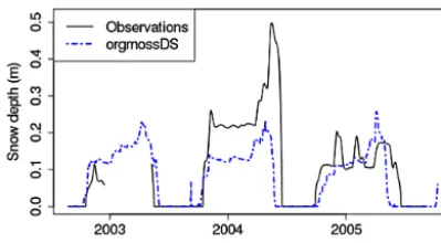
Figure 7. Simulated and observed snow depth at Samoylov over
the same years as soil temperatures (Fig. 6b). The simulation orgmossDS includes all model improvements (see Table 1).
soil temperatures are simulated fairly accurately, the snow depth is below that observed, whilst in winter 2004–2005 the snow depth is close to the observations but the soil temper-atures are too warm. This suggests that the simulated snow density is too low. The snow density determines the thermal conductivity which, combined with the snow depth, is used to calculate the heat flow between air and soil.
A further simulation was performed, increasing the fresh snow density even more from 130 to 170 kg m−3 (see Ta-ble 1). This increased the mean snow density that was sim-ulated in JULES from around 190 to 220 kg m−3, which matches more closely with the observational estimate specif-ically for polygon centres, which is about 230 kg m−3(Boike et al., 2013).
Figure 8 shows the effect of increasing snow density. The soil is now too cold in winter 2003–2004, which is consis-tent with there being too little snow. In winter 2004–2005, where snow depths are more realistic, the soil temperatures match better with those observed. During the coldest months (January–March) there is a strong correlation of approxi-mately 0.85 between the error in snow depth and the error in soil temperature, for both simulations. However, the lin-ear regression line crosses a long way above the origin in orgmossDS (4.3◦C), whereas when the fresh snow density is higher it passes closer to the origin (1.8◦C) – see Fig. 8. For these months, usingρfresh=170 kg m−3reduces the RMSE in soil temperature from 3.9 to 2.4◦C. However, the whole-year RMSE in soil temperature is increased from 3.4 to 3.7◦C, mainly because of differences in temperatures in the shoulder seasons, in particular during the freeze-up period in autumn, when the simulated zero-curtain length is too short (the zero curtain is the period for which the soil remains at or close to 0◦C during freeze or thaw). The end of the freeze-up happens on average 30 days too early in orgmossDS, and when the snow density is increased it is even earlier, on aver-age 42 days before the observed freeze-up date.
The zero-curtain duration is determined by the latent heat associated with freeze–thaw. In reality, polygon centres tend to be saturated (Boike et al., 2013). If there is not enough
soil moisture, some latent heat will be missing, reducing the zero-curtain length. Figure 9 compares the volumet-ric soil moisture content in the observations and simula-tions. It is clearly improved in the organic soil simulations (orgmossD, orgmossDS) compared to the mineral soil sim-ulations (min4l, minD), but there is still too little soil mois-ture, partly because the porosity is too low and partly because the soil does not always stay saturated. The offset timings of freeze and thaw are clearly seen, showing that the timing of thaw is greatly improved in orgmossD and orgmossDS, but there is little effect on the time of the freeze. Note that the unfrozen soil moisture content in winter is higher than the observations, which suggests the hydraulic parameters may need some refinement.
In order to investigate the soil moisture effect, a simulation was performed in which the soil was kept saturated all year-round, and the organic matter content in the upper soil layers was increased to 45 kg m−3to increase the porosity to match better with the observations (Saturated in Table 1). As a re-sult, the thermal conductivity and heat capacity generally fall within the uncertainty of the values in Langer et al. (2011a, b), although the frozen heat capacity is increased with a max-imum value of 2.4 MJ m−3K−1, which is 20 % greater than the values in Langer et al. (2011b). The simulation results are shown in Fig. 10.
Figure 10 shows a great improvement in the zero-curtain length, with the mean difference between the simulated and observed freeze-up now being only 13 days (instead of 30 in orgmossDS). The overall RMSE for the upper soil tempera-tures is reduced further from 3.4 to 2.7◦C, and the deep soil temperatures are also improved (see Saturated in Table 2). The summer soil temperatures are actually a little warmer and in fact this reduces the RMSE for August–September temperatures (at 32 cm) slightly from 0.7 to 0.6◦C. Fig-ure 10a shows that the time series of unfrozen soil moistFig-ure is also greatly improved. These improvements highlight the need for more work on soil hydrology.
Figure 8. Effect of increasing the fresh snow density (ρfresh) from 130 to 170 kg m−3for the simulation set-up orgmossDS (Table 1). The lower plot compares the error in soil temperatures and snow depths for the coldest months only (January–March) using daily values.
Figure 9. Simulated and observed soil moisture at approximately
32 cm depth. The simulations include the standard JULES set-up (min4l) and show the effects of a deeper and better-resolved soil (minD), adding organic soils and moss (orgmossD) and improving the snow scheme (orgmossDS). Observations are from a polygon centre.
site. This would give more snow insulation during the freeze-up period, but the simulated mid-winter snow density in JULES would then be too low. This could be addressed by in-cluding compaction processes in the model that are currently not represented, such as wind compaction and temperature-gradient metamorphosis, both of which are potentially im-portant (Sturm and Holmgren, 1998; Vionnet et al., 2012).
4 Conclusions and future work
Improvements have been made to the physical representation of permafrost in the JULES land-surface model. Additional processes represented include an insulating moss layer, the physical properties of organic soil, and a bedrock column. In addition, the representation of snow and discretisation of the soil have been modified.
These developments are extremely relevant for the Arctic in general, since soils in the continuous permafrost zone are often organic-rich and covered by moss, which is certainly the case at Samoylov Island, where we run the model simu-lations. It is therefore important to include these processes in global land-surface models.
Figure 10. Simulated and observed (a) soil moisture and (b) temperatures at approximately 32 cm depth. Unfrozen soil moisture is
shown as a fraction of saturation. The three simulations show firstly the effect of increasing snow density (compare orgmossDS and ρfresh=170 kg m−3) and the effect of setting the soil moisture to saturated with increased organic matter (compareρfresh=170 kg m−3 and Saturated). Observations are from a polygon centre.
In the shoulder seasons, the zero-curtain duration is strongly related to soil moisture. This requires further work in JULES, as the model does not obtain the saturated condi-tions observed in the field. The relevance of this is seen by fixing the soil moisture in the saturated simulation, which al-ters the timing of freeze-up from 30 days to only 13 days too early.
Snow is the most important process for winter soil temper-atures, which can be seen here by the high correlation (0.85) between soil temperature error and snow depth error in the winter months. Soil temperatures are particularly sensitive to shallow snow; hence, our improvement to the snow model is essential for simulating soil temperatures in the shoulder seasons. The snow on Samoylov Island is shallow and highly wind-blown, which is typical of these low-lying tundra re-gions. We find that the fresh snow density required to obtain the correct mid-winter snow density in JULES is too high, in-dicating a need for further work, potentially to include more snow compaction processes.
Another area for future development is the vegetation, since there are currently no specific high-latitude PFT’s in JULES. The moss cover represented here is a first step to-wards simulating tundra vegetation; however, this represents only the physical effects of a constant layer of moss, leav-ing more work to be done, for example on growth, carbon cycling, and on other types of vegetation.
Appendix A: Details of organic soil parameterisation Using an organic fraction, forg, organic and mineral soil properties are combined as follows:
b=(1−forg)bm+forgbo, (A1) ψsat=ψ
1−forg
sat,m ψ forg
sat,o, (A2)
Ks=K 1−forg
s,m K
forg
s,o , (A3)
θsat=(1−forg)θsat,m+forgθsat,o, (A4) θcrit=θsat
ψ
sat 3.364
1/b
, (A5)
θwilt=θsat
ψ
sat 152.9
1/b
, (A6)
Cdry=(1−forg)Cdry,m+forgCdry,o, (A7) λdry=λ
1−forg
dry,m λ forg
dry,o. (A8)
Subscripts m and o denote values for mineral and organic soils, respectively.Ks is the hydraulic conductivity at satu-ration,θcritandθwiltare the moisture contents for the critical point and wilting point, andCdryandλdryare thermal proper-ties: heat capacity and thermal conductivity of dry soil. The properties for organic soils are as in Dankers et al. (2011) (Table 2). Some of these parameters are given as three differ-ent values for differdiffer-ent vertical layers of the soil. The division between layers was taken at 0.3 and 1 m.
While the dry thermal conductivity, λdry, is input to JULES, the saturated thermal conductivity is calculated in the model. The preferred parameterisation of saturated ther-mal conductivity in the standard version of JULES (Dharssi et al., 2009) is as follows:
λsat=λsat0 λfwatθsat
wat λ ficeθsat
ice
λθsat
wat
, (A9)
where
fwat=θu/(θu+θf);fice=θf/(θu+θf),
where θu is the volumetric unfrozen water content and θf is the volumetric frozen water content.λsat0 is the saturated thermal conductivity when the soil is entirely unfrozen, given by
λsat0= (A10)
( 1.58 λ
dry<0.25 (1.58+12.4(λdry−0.25)) 0.25< λdry<0.3
2.2 λdry>0.3
)
Wm−1K−1.
This parameterisation is replaced with the following equa-tion, which allows the saturated conductivity to take lower values appropriate to organic soils:
λsat0= (A11)
0.5 λdry<0.06 1.0−0.0134 ln(λdry)
−0.745−ln(λdry) 0.06< λdry<0.3
2.2 λdry>0.3
Wm−1K−1.
Code availability
The model developments are available in JULES branches created by S. Chadburn (sec234) and E. Burke (hadea) on PUMA (https://puma.nerc.ac.uk/svn/JULES_svn/JULES/ branches/dev/). A password can be requested for access (see https://jules.jchmr.org). If you would like us to send you the code, please contact us.
Author contributions. S. Chadburn and E. Burke developed moss,
organic soil and bedrock representations in the model. R. Essery developed the improved snow scheme. J. Boike, M. Langer and M. Heikenfeld provided field data, images and knowledge of the Samoylov Island site. P. Friedlingstein and P. Cox provided initial ideas and oversight. S. Chadburn ran the simulations and wrote up the results.
Acknowledgements. The authors acknowledge financial support by
the European Union Seventh Framework Programme (FP7/2007– 2013) project PAGE21, under GA282700. E. J. Burke was supported by the Joint UK DECC/Defra Met Office Hadley Centre Climate Programme GA01101. M. Langer is also supported by a post-doctoral research fellowship (A. v. Humboldt Foundation). Work was facilitated by a PAGE21 young researcher exchange grant. Thanks go to the Russian–German expedition team for logistical support during the Samoylov field work. Thanks to Niko Bornemann, Steffen Frey and Günter Stoof for data collection and compilation.
Edited by: D. Lawrence
References
Alexeev, V. A., Nicolsky, D. J., Romanovsky, V. E., and Lawrence, D. M.: An evaluation of deep soil configurations in the CLM3 for improved representation of permafrost, Geophys. Res. Lett., 34, L09502, doi:10.1029/2007GL029536, 2007. Bekryaev, R. V., Polyakov, I. V., and Alexeev, V. A.: Role of
polar amplification in long-term surface air temperature varia-tions and modern Arctic warming, J. Climate, 23, 3888–3906, doi:10.1175/2010JCLI3297.1, 2010.
Beringer, J., Lynch, A. H., Chapin, F. S., Mack, M., and Bo-nan, G. B.: The representation of Arctic soils in the land surface model: the importance of mosses, J. Climate, 14, 3324–3335, doi:10.1175/1520-0442(2001)014<3324:TROASI>2.0.CO;2, 2001.
Best, M. J., Pryor, M., Clark, D. B., Rooney, G. G., Essery, R .L. H., Ménard, C. B., Edwards, J. M., Hendry, M. A., Porson, A., Gedney, N., Mercado, L. M., Sitch, S., Blyth, E., Boucher, O., Cox, P. M., Grimmond, C. S. B., and Harding, R. J.: The Joint UK Land Environment Simulator (JULES), model description – Part 1: Energy and water fluxes, Geosci. Model Dev., 4, 677–699, doi:10.5194/gmd-4-677-2011, 2011.
Boike, J., Kattenstroth, B., Abramova, K., Bornemann, N., Chetverova, A., Fedorova, I., Fröb, K., Grigoriev, M.,
Grüber, M., Kutzbach, L., Langer, M., Minke, M., Muster, S., Piel, K., Pfeiffer, E.-M., Stoof, G., Westermann, S., Wis-chnewski, K., Wille, C., and Hubberten, H.-W.: Baseline characteristics of climate, permafrost and land cover from a new permafrost observatory in the Lena River Delta, Siberia (1998–2011), Biogeosciences, 10, 2105–2128, doi:10.5194/bg-10-2105-2013, 2013.
Brooks, R. and Corey, A.: Hydraulic Properties of Porous Me-dia, Colorado State University Hydrology Papers, Colorado State University, available at: http://books.google.co.uk/books?id=F_ 1HOgAACAAJ (last access: 27 January 2015), 1964.
Brown, J., Ferrians Jr, O. J., Heginbottom, J., and Melnikov, E.: Circum-arctic map of permafrost and ground ice conditions, Na-tional Snow and Ice Data Center, available at: http://nsidc.org/ data/docs/fgdc/ggd318_map_circumarctic (last access: 27 Jan-uary 2015), 1998.
Brown, J., Nelson, F. E., and Hinkel, K. M.: The circumpolar active layer monitoring (CALM) program: research designs and initial results, Polar Geography, 3, 165–258, 2000.
Burke, E., Dankers, R., Jones, C., and Wiltshire, A.: A retrospective analysis of pan Arctic permafrost using the JULES land surface model, Clim. Dynam., 41, 1025–1038, doi:10.1007/s00382-012-1648-x, 2013.
Burke, E. J., Hartley, I. P., and Jones, C. D.: Uncertainties in the global temperature change caused by carbon release from per-mafrost thawing, The Cryosphere, 6, 1063–1076, doi:10.5194/tc-6-1063-2012, 2012.
Camill, P.: Permafrost thaw accelerates in boreal peatlands during late-20th century climate warming, Climatic Change, 68, 135– 152, doi:10.1007/s10584-005-4785-y, 2005.
Chadburn, S. E., Burke, E. J., Essery, R. L. H., Boike, J., Langer, M., Heikenfeld, M., Cox, P. M., and Friedlingstein, P.: Impact of model developments on present and future simulations of per-mafrost in a global land-surface model, The Cryosphere Discuss., 9, 1965–2012, doi:10.5194/tcd-9-1965-2015, 2015.
Christensen, T. R. and Cox, P.: Response of methane emission from arctic tundra to climatic change: results from a model simulation, Tellus B, 47, 301–309, doi:10.1034/j.1600-0889.47.issue3.2.x, 1995.
Clark, D. B., Mercado, L. M., Sitch, S., Jones, C. D., Gedney, N., Best, M. J., Pryor, M., Rooney, G. G., Essery, R. L. H., Blyth, E., Boucher, O., Harding, R. J., Huntingford, C., and Cox, P. M.: The Joint UK Land Environment Simulator (JULES), model descrip-tion – Part 2: Carbon fluxes and vegetadescrip-tion dynamics, Geosci. Model Dev., 4, 701–722, doi:10.5194/gmd-4-701-2011, 2011. Cosby, B. J., Hornberger, G. M., Clapp, R. B., and Ginn, T. R.: A
statistical exploration of the relationships of soil moisture char-acteristics to the physical properties of soils, Water Resour. Res., 20, 682–690, doi:10.1029/WR020i006p00682, 1984.
Cox, P. M.: Description of the TRIFFID Dynamic Global Vegeta-tion Model, Hadley Centre Technical Note 24, Hadley Centre, Met Office, Bracknell, UK, 2001.
Cox, P. M., Betts, R. A., Bunton, C. B., Essery, R. L. H., Rown-tree, P. R., and Smith, J.: The impact of new land surface physics on the GCM simulation of climate and climate sensitivity, Clim. Dynam., 15, 183–203, doi:10.1007/s003820050276, 1999. Dankers, R., Burke, E. J., and Price, J.: Simulation of permafrost
Dharssi, I., Vidale, P., Verhoef, A., Macpherson, B., Jones, C., and Best, M.: New soil physical properties implemented in the Unified Model at PS18, Meteorology Research and Development technical report 528, Met. Office, UK, available at: http://www.metoffice.gov.uk/archive/ forecasting-research-technical-report-528 (last access: 27 Jan-uary 2015), 2009.
Dyrness, C.: Control of depth to permafrost and soil temperature by the forest floor in black spruce/feathermoss communities, Pacific Northwest Forest and Range Experiment Station (Portland, Or.), 396, 1982.
ECMWF (European Center for Medium-Range Weather Fore-casts): ECMWF ERA-40 Re-Analysis data, NCAS British At-mospheric Data Centre, available at: http://badc.nerc.ac.uk/view/ badc.nerc.ac.uk__ATOM__dataent_ECMWF-E40 (last access: 27 January 2015), 2006.
ECMWF (European Center for Medium-Range Weather Forecasts): ERA-Interim project, Research Data Archive at the National Center for Atmospheric Research, Computational and Informa-tion Systems Laboratory, available at: http://dx.doi.org/10.5065/ D6CR5RD9 (last access: 28 April 2015), 2009.
Ekici, A., Beer, C., Hagemann, S., Boike, J., Langer, M., and Hauck, C.: Simulating high-latitude permafrost regions by the JSBACH terrestrial ecosystem model, Geosci. Model Dev., 7, 631–647, doi:10.5194/gmd-7-631-2014, 2014a.
Ekici, A., Chadburn, S., Chaudhary, N., Hajdu, L. H., Marmy, A., Peng, S., Boike, J., Burke, E., Friend, A. D., Hauck, C., Krin-ner, G., Langer, M., Miller, P. A., and Beer, C.: Site-level model intercomparison of high latitude and high altitude soil thermal dynamics in tundra and barren landscapes, The Cryosphere Dis-cuss., 8, 4959–5013, doi:10.5194/tcd-8-4959-2014, 2014b. Essery, R. and Pomeroy, J.: Vegetation and topographic
control of wind-blown snow distributions in distributed and aggregated simulations for an Arctic tundra basin, J. Hydrometeorol., 5, 735–744, doi:10.1175/1525-7541(2004)005<0735:VATCOW>2.0.CO;2, 2004.
Essery, R., Best, M., Betts, R., and Taylor, C.: Explicit representa-tion of subgrid heterogeneity in a GCM land surface scheme, J. Hydrometeorol., 4, 530–543, 2003.
Exbrayat, J.-F., Pitman, A. J., Zhang, Q., Abramowitz, G., and Wang, Y.-P.: Examining soil carbon uncertainty in a global model: response of microbial decomposition to temperature, moisture and nutrient limitation, Biogeosciences, 10, 7095– 7108, doi:10.5194/bg-10-7095-2013, 2013.
Gedney, N. and Cox, P. M.: The sensitivity of global cli-mate model simulations to the representation of soil mois-ture, J. Hydrometeorol., 4, 1265–1275, doi:10.1175/1525-7541(2003)004<1265:TSOGCM>2.0.CO;2, 2003.
Gouttevin, I., Krinner, G., Ciais, P., Polcher, J., and Legout, C.: Multi-scale validation of a new soil freezing scheme for a land-surface model with physically-based hydrology, The Cryosphere, 6, 407–430, doi:10.5194/tc-6-407-2012, 2012a.
Gouttevin, I., Menegoz, M., Dominé, F., Krinner, G., Koven, C., Ciais, P., Tarnocai, C., and Boike, J.: How the insulating prop-erties of snow affect soil carbon distribution in the continen-tal pan-Arctic area, J. Geophys. Res.-Biogeo., 117, G02020, doi:10.1029/2011JG001916, 2012b.
Jafarov, E. E., Marchenko, S. S., and Romanovsky, V. E.: Numerical modeling of permafrost dynamics in Alaska using a high spatial
resolution dataset, The Cryosphere, 6, 613–624, doi:10.5194/tc-6-613-2012, 2012.
Khvorostyanov, D. V., Ciais, P., Krinner, G., and Zi-mov, S. A.: Vulnerability of east Siberia’s frozen carbon stores to future warming, Geophys. Res. Lett., 35, L10703, doi:10.1029/2008GL033639, 2008.
Koven, C., Friedlingstein, P., Ciais, P., Khvorostyanov, D., Krin-ner, G., and Tarnocai, C.: On the formation of high-latitude soil carbon stocks: effects of cryoturbation and insulation by organic matter in a land surface model, Geophys. Res. Lett., 36, L21501, doi:10.1029/2009GL040150, 2009.
Koven, C. D., Ringeval, B., Friedlingstein, P., Ciais, P., Cadule, P., Khvorostyanov, D., Krinner, G., and Tarnocai, C.: Permafrost carbon–climate feedbacks accelerate global warming, P. Natl. Acad. Sci. USA, doi:10.1073/pnas.1103910108, 2011.
Koven, C. D., Riley, W. J., and Stern, A.: Analysis of per-mafrost thermal dynamics and response to climate change in the CMIP5 earth system models, J. Climate, 26, 1877–1900, doi:10.1175/JCLI-D-12-00228.1, 2012.
Langer, M., Westermann, S., Muster, S., Piel, K., and Boike, J.: The surface energy balance of a polygonal tundra site in north-ern Siberia – Part 1: Spring to fall, The Cryosphere, 5, 151–171, doi:10.5194/tc-5-151-2011, 2011a.
Langer, M., Westermann, S., Muster, S., Piel, K., and Boike, J.: The surface energy balance of a polygonal tundra site in north-ern Siberia – Part 2: Winter, The Cryosphere, 5, 509–524, doi:10.5194/tc-5-509-2011, 2011b.
Langer, M., Westermann, S., Heikenfeld, M., Dorn, W., and Boike, J.: Satellite-based modeling of permafrost temperatures in a tundra lowland landscape, Remote Sens. Environ., 135, 12– 24, doi:10.1016/j.rse.2013.03.011, 2013.
Lawrence, D. and Slater, A.: Incorporating organic soil into a global climate model, Clim. Dynam., 30, 145–160, doi:10.1007/s00382-007-0278-1, 2008.
Lawrence, D., Slater, A., Romanovsky, V., and Nicolsky, D.: Sensi-tivity of a model projection of near-surface permafrost degrada-tion to soil column depth and representadegrada-tion of soil organic mat-ter, J. Geophys. Res., 113, F02011, doi:10.1029/2007JF000883, 2008.
Lawrence, D. M., Slater, A. G., and Swenson, S. C.: Simula-tion of present-day and future permafrost and seasonally frozen ground conditions in CCSM4, J. Climate, 25, 2207–2225, doi:10.1175/JCLI-D-11-00334.1, 2012.
Mitchell, T. D. and Jones, P. D.: An improved method of con-structing a database of monthly climate observations and as-sociated high-resolution grids, Int. J. Climatol., 25, 693–712, doi:10.1002/joc.1181, 2005.
Muster, S., Langer, M., Heim, B., Westermann, S., and Boike, J.: Subpixel heterogeneity of ice-wedge polygonal tundra: a multi-scale analysis of land cover and evapotranspiration in the Lena River Delta, Siberia, Tellus B, 64, 17301, doi:10.3402/tellusb.v64i0.17301, 2012.
Overland, J. E., Spillane, M. C., Percival, D. B., Wang, M., and Mofjeld, H. O.: Seasonal and regional variation of pan-arctic surface air temperature over the instrumen-tal record, J. Climate, 17, 3263–3282, doi:10.1175/1520-0442(2004)017<3263:SARVOP>2.0.CO;2, 2004.
Rinke, A., Kuhry, P., and Dethloff, K.: Importance of a soil organic layer for Arctic climate: a sensitivity study with an Arctic RCM, Geophys. Res. Lett., 35, L13709, doi:10.1029/2008GL034052, 2008.
Riseborough, D., Shiklomanov, N., Etzelmüller, B., Gruber, S., and Marchenko, S.: Recent advances in permafrost modelling, Per-mafrost Periglac., 19, 137–156, doi:10.1002/ppp.615, 2008. Romanovsky, V. E., Drozdov, D. S., Oberman, N. G.,
Malkova, G. V., Kholodov, A. L., Marchenko, S. S., Moskalenko, N. G., Sergeev, D. O., Ukraintseva, N. G., Abramov, A. A., Gilichinsky, D. A., and Vasiliev, A. A.: Thermal state of permafrost in Russia, Permafrost Periglac., 21, 136–155, doi:10.1002/ppp.683, 2010.
Romanovsky, V. E., Smith, S. L., Christiansen, H. H., Shiklo-manov, N. I., Streletskiy, D. A., Drozdov, D. S., Oberman, N. G., Kholodov, A. L., and Marchenko, S. S.: Permafrost (Arc-tic Report Card 2013) available at: http://www.arc(Arc-tic.noaa.gov/ reportcard (last access: 27 January 2015), 2013.
Schaphoff, S., Heyder, U., Ostberg, S., Gerten, D., Heinke, J., and Lucht, W.: Contribution of permafrost soils to the global car-bon budget, Environ. Res. Lett., 8, 014026, doi:10.1088/1748-9326/8/1/014026, 2013.
Schneider von Deimling, T., Meinshausen, M., Levermann, A., Hu-ber, V., Frieler, K., Lawrence, D. M., and Brovkin, V.: Estimating the near-surface permafrost-carbon feedback on global warming, Biogeosciences, 9, 649–665, doi:10.5194/bg-9-649-2012, 2012. Soudzilovskaia, N. A., van Bodegom, P. M., and Cornelissen, J. H.: Dominant bryophyte control over high-latitude soil tempera-ture fluctuations predicted by heat transfer traits, field moistempera-ture regime and laws of thermal insulation, Funct. Ecol., 27, 1442– 1454, doi:10.1111/1365-2435.12127, 2013.
Stevens, M. B., Smerdon, J. E., González-Rouco, J. F., Stieglitz, M., and Beltrami, H.: Effects of bottom boundary placement on sub-surface heat storage: implications for climate model simulations, Geophys. Res. Lett., 34, L02702, doi:10.1029/2006GL028546, 2007.
Stocker, T., Qin, D., Plattner, G.-K., Tignor, M., Allen, S., Boschung, J., Nauels, A., Xia, Y., Bex, V., and Midgley, P. M. (Eds.): Climate Change 2013: The Physical Science Ba-sis. Contribution of Working Group I to the Fifth Assessment Report of the Intergovernmental Panel on Climate Change, IPCC, Cambridge University Press, available at: http://www. climatechange2013.org/ (last access: 27 January 2015), 2013. Sturm, M. and Holmgren, J.: Differences in compaction behavior of
three climate classes of snow, Ann. Glaciol., 26, 125–130, 1998.
Tarnocai, C., Canadell, J. G., Schuur, E. A. G., Kuhry, P., Mazhi-tova, G., and Zimov, S.: Soil organic carbon pools in the north-ern circumpolar permafrost region, Global Biogeochem. Cy., 23, GB2023, doi:10.1029/2008GB003327, 2009.
Tian, W., Li, X., Cheng, G.-D., Wang, X.-S., and Hu, B. X.: Cou-pling a groundwater model with a land surface model to improve water and energy cycle simulation, Hydrol. Earth Syst. Sci., 16, 4707–4723, doi:10.5194/hess-16-4707-2012, 2012.
Vionnet, V., Brun, E., Morin, S., Boone, A., Faroux, S., Le Moigne, P., Martin, E., and Willemet, J.-M.: The detailed snowpack scheme Crocus and its implementation in SURFEX v7.2, Geosci. Model Dev., 5, 773–791, doi:10.5194/gmd-5-773-2012, 2012.
Weedon, G. P.: Readme file for the “WFDEI” dataset, avail-able at: http://www.eu-watch.org/gfx_content/documents/ README-WFDEI.pdf (last access: 27 January 2015), 2013. Weedon, G. P., Gomes, S., Viterbo, P., Österle, H., Adam, J. C.,
Bellouin, N., Boucher, O., and Best., M.: The WATCH forc-ing data 1958–2001: a meteorological forcforc-ing dataset for land surface- and hydrological-models., WATCH technical report, p. 41, available at: http://www.eu-watch.org/publications (last access: 27 January 2015), 2010.
Weedon, G. P., Gomes, S., Viterbo, P., Shuttleworth, W. J., Blyth, E., Österle, H., Adam, J. C., Bellouin, N., Boucher, O., and Best, M.: Creation of the WATCH forcing data and its use to assess global and regional reference crop evaporation over land dur-ing the twentieth century, J. Hydrometeorol., 12, 823–847, doi:10.1175/2011JHM1369.1, 2011.
Westermann, S., Schuler, T. V., Gisnås, K., and Etzelmüller, B.: Transient thermal modeling of permafrost conditions in South-ern Norway, The Cryosphere, 7, 719–739, doi:10.5194/tc-7-719-2013, 2013.
Westermann, S., Elberling, B., Højlund Pedersen, S., Stendel, M., Hansen, B. U., and Liston, G. E.: Future permafrost conditions along environmental gradients in Zackenberg, Greenland, The Cryosphere, 9, 719–735, doi:10.5194/tc-9-719-2015, 2015. Williams, P. and Smith, M.: The Frozen Earth:
Fundamen-tals of Geocryology, Studies in Polar Res., Cambridge Uni-versity Press, available at: http://books.google.co.uk/books?id= YYCvQAAACAAJ (last access: 27 January 2015), 1991. Yi, S., Wischnewski, K., Langer, M., Muster, S., and Boike, J.:
Freeze/thaw processes in complex permafrost landscapes of northern Siberia simulated using the TEM ecosystem model: im-pact of thermokarst ponds and lakes, Geosci. Model Dev., 7, 1671–1689, doi:10.5194/gmd-7-1671-2014, 2014.