https://doi.org/10.5194/gmd-11-2153-2018 © Author(s) 2018. This work is distributed under the Creative Commons Attribution 4.0 License.
Automated model optimisation using the Cylc workflow
engine (Cyclops v1.0)
Richard M. Gorman1and Hilary J. Oliver2
1National Institute of Water and Atmospheric Research, P.O. Box 11-115, Hamilton, New Zealand 2National Institute of Water and Atmospheric Research, Private Bag 14901, Wellington, New Zealand
Correspondence:Richard M. Gorman ([email protected]) Received: 3 August 2017 – Discussion started: 21 September 2017 Revised: 3 May 2018 – Accepted: 20 May 2018 – Published: 12 June 2018
Abstract. Most geophysical models include many param-eters that are not fully determined by theory, and can be “tuned” to improve the model’s agreement with available data. We might attempt to automate this tuning process in an objective way by employing an optimisation algorithm to find the set of parameters that minimises a cost function de-rived from comparing model outputs with measurements. A number of algorithms are available for solving optimisation problems, in various programming languages, but interfacing such software to a complex geophysical model simulation presents certain challenges.
To tackle this problem, we have developed an optimisa-tion suite (“Cyclops”) based on the Cylc workflow engine that implements a wide selection of optimisation algorithms from the NLopt Python toolbox (Johnson, 2014). The Cy-clops optimisation suite can be used to calibrate any mod-elling system that has itself been implemented as a (sepa-rate) Cylc model suite, provided it includes computation and output of the desired scalar cost function. A growing num-ber of institutions are using Cylc to orchestrate complex dis-tributed suites of interdependent cycling tasks within their operational forecast systems, and in such cases application of the optimisation suite is particularly straightforward.
As a test case, we applied the Cyclops to calibrate a global implementation of the WAVEWATCH III (v4.18) third-generation spectral wave model, forced by ERA-Interim in-put fields. This was calibrated over a 1-year period (1997), before applying the calibrated model to a full (1979–2016) wave hindcast. The chosen error metric was the spatial av-erage of the root mean square error of hindcast significant wave height compared with collocated altimeter records. We
describe the results of a calibration in which up to 19 param-eters were optimised.
1 Introduction
Geophysical models generally include some empirical pa-rameterisations that are not fully determined by physical theory and which need calibration. The calibration process has often been somewhat subjective and poorly documented (Voosen, 2016) but in a more objective approach has the aim of minimising some measure of error quantified from com-parisons with measurement (Hourdin et al., 2017). We can turn this into an optimisation problem: namely, to find the minimum of an objective functionf (x), wherex represents the set of adjustable parameters, andf is a single error met-ric (e.g. the sum of RMS differences between measured and predicted values of a set of output variables) resulting from a model simulation with that parameter set.
The most efficient optimisation algorithms require the derivative∇f (x)to be available alongsidef (x). This, how-ever, is rarely the case for a geophysical modelling system, so we will restrict our attention to the field of differential free optimisation (DFO), in which the objective functionfcan be calculated, but its gradient is not available.
require the user to supply a subroutine to computef (x), that can be called as required by the optimisation programme.
This is satisfactory for many problems where the objec-tive function is readily expressed as an algorithm but is somewhat less straightforward to interface an existing geo-physical model, as well as all the methods needed to pro-cess and compare measurement data with an optimisation code, in this way. Nevertheless, examples of this approach can be found in hydrological and climate modelling appli-cations. For example, Seong et al. (2015) developed a cal-ibration tool (using R software) to apply the shuffled com-plex evolution optimisation algorithm to calibrate the Hydro-logic Simulation Program–Fortran (HSPF) model. In climate modelling, Severijns and Hazeleger (2005) used the down-hill simplex method to optimise the parameter values of the subgrid parameterisations of an atmospheric general circula-tion model. More recently, Tett et al. (2013) applied a Gauss– Newton line search optimisation algorithm to climate simu-lations with the Hadley Centre Atmosphere Model version 3 (HadAM3) forced with observed sea surface temperature and sea ice, optimising an objective function derived from re-flected shortwave radiation and outgoing longwave radiation comparisons. The Tett et al. (2013) method was subsequently applied to optimise the sea ice component of the global cou-pled HadCM3 climate model (Roach et al., 2017; Tett et al., 2017).
Such custom applications of one particular optimisation algorithm to a specific model, however, can require signifi-cant effort to switch to alternative optimisation algorithms or to be applied to new models. Modern coupled climate mod-els, or operational forecast systems for weather and related processes, encompass a diverse set of software tools, often running on multiple platforms. Ideally, we would like to be able to optimise performance of the modelling system (not just a single model code) without major reconfiguration of software between the calibration and operational/production versions of the system.
The Cylc workflow engine is now applied in several oper-ational centres to manage the scheduling of tasks within such systems. So it seems natural to consider the possibility of de-veloping a framework within Cylc for the optimisation of the modelling systems under its control.
2 Methods
In very general terms, a derivative-free optimisation algo-rithm will explore parameter space, selecting values of the parameter vectorxin some sequence. As eachxis selected, it calls the (user-supplied) subroutine to evaluate the objec-tive functionf (x). In our case, this would amount to running a complete model simulation with the corresponding parame-ter settings, comparing outputs to measurements, from which a defined error metric is computed to provide the return value of f. This can involve a lengthy simulation, needing a run
timeTmodel perhaps of the order of hours or days to
repro-duce months or years of measurements.
A self-contained optimisation programme, with an ex-plicitly coded function-evaluation subroutine, will run much faster, with a run time per iterationTitertypically being some
small fraction of a second, and will run in many orders of magnitude less time than a typical geophysical model even if a number of iterationsN of order 1000 are required. This might be the case for “deliberately difficult” test problems: we might expect that a well-tested geophysical model will come with reasonable defaults that in many new implemen-tations will produce a result within a relatively simple “basin of attraction” so thatO(10)iterations may suffice to get very close.
If the optimisation procedure calls for a full model run to evaluate the objective function, andNiterations are required for convergence, the total run time would be
T ≈To+N (Tmodel+Titer), (1)
including an overheadTofor initial and final tasks.
As Tmodel is orders of magnitude larger than To and
Titer, the geophysical modelling system totally dominates run
time, and we can comfortably afford not to be concerned with reducing the efficiency of the optimisation routine, even by a few orders of magnitude.
So let us consider a simple measure we might introduce to allow us to recover from an interruption part of the way through a long optimisation process. Normally, the optimi-sation code will retain in memory the values of eachx and its objective functionf (x)that has already been evaluated, to use in selecting further points to be evaluated. If we write these values to file each time the function evaluation is called, we can build up a lookup table to use in case we need to restart the process. In that case, we could have the func-tion evaluafunc-tion subroutine first search the lookup table for a match to x (within some acceptable tolerance), in which case it could return the tabulated error value. Only in the case where a tabulated value was not found would the full model simulation be required to compute the return value off.
Now rather than actually perform that computation, the function evaluation subroutine could simply write thex val-ues (for thenth iteration, for instance) to file, and exit. We could then run the model in its usual way, outside the optimi-sation code, using thosexvalues as parameters, and add that result to our lookup table before restarting the whole process from scratch. This time, assuming the optimisation algorithm is deterministic, with no random process influencing the se-quence ofx values, the firstnpoints would be exactly the same sequence that was selected previously, and could be quickly handled by table lookup, and the algorithm would either find that a convergence criterion had been satisfied, or select a new pointn+1 to be passed to the model for simula-tion.
iterations, either signals that convergence has been reached or generates the next parameter set to be evaluated by the model, i.e.
xn+1=Opt({xm, fm}m=1,...,n). (2) In this scheme, assuming that we start with an empty lookup table, the first pass has one iteration of the optimisa-tion code, the second has two, etc. So, allowing an addioptimisa-tional overhead Tˆ for the full process, the total run time to reach the termination condition(s) afterN iterations should be
T0= ˆT+ N X
n=1
(To+nTiter+Tmodel) (3)
= ˆT+N (To+Tmodel)+
N (N+1)
2 Titer. (4)
As Tmodel is orders of magnitude larger than the other
times, the ratio of the two run times is T0
T ≈1+ N+1
2 Titer
Tmodel
. (5)
Given the expected relative magnitudes of the model and optimisation iteration times, andN of order 10 or 100 s, the increase in run time through this approach is actually negli-gible.
On the other hand, this scheme has several benefits. Apart from being simple to code, the optimisation algorithm, in-cluding the user-defined function evaluation subroutine, can be completely generic, and applied unmodified to different modelling systems. The only requirements on the modelling system are that, at the start of each simulation, it reads in the parameter values requested by the optimisation code and adapt them to its standard input formats, then at the end of the simulation, computes and writes to file a single error metric value. The optimisation code and the model system could then remain separate, both controlled by some form of scripting scheme, for example. This means that having in-vested considerable time and resources in developing a com-plex modelling scheme, no major reconfiguration needs to be made to prepare it for optimisation in this manner or subse-quently to re-implement the optimised modelling system in operational or production mode.
2.1 Cylc
Cylc (http://cylc.github.io/cylc/) is an open-source workflow engine that can manage ongoing distributed workflows of cy-cling (repeating) tasks. It was originally developed at the Na-tional Institute of Water and Atmospheric Research (NIWA) to automate environmental forecasting systems and has since been adopted by many other institutions – notably the UK Met Office and its international partners in climate, weather and related sciences. Cylc can manage large production sys-tems of great complexity, but it is also easy to use for
indi-viduals and groups with less demanding automation require-ments. Cylc workflows (or suites) are defined with an effi-cient graph syntax that expresses dependence between tasks and an efficient inheritance hierarchy for optimal sharing of all task run time properties (exactly what each task should execute, and where and how to submit task jobs to run).
Cylc tasks are related by trigger expressions that combine to form a dependency graph. This trigger,
A:status=>B
says that task B depends on task A achieving the sta-tus status(“=>” represents an arrow). The default trigger status issucceeded (job execution completed successfully) and can be written simply as A=> B; others include submitted, submit-failed, started, finished, failedand custom task output messages. Tasks can depend on the wall clock and on external events, as well as on other tasks, and a task job can be submitted to run once all its dependencies are met. Cylc automatically wraps user-defined task content (environment, scripting, etc.) in code to trap errors and report job status back to the suite server programme via authenticated HTTPS messages. Tasks can even trigger off tasks in other suites, so for coupled systems you can choose between a larger suite that controls all tasks and multiple smaller suites that interact with each other.
In cycling systems, tasks repeat on sequences that may represent forecast cycles or separate chunks of a model sim-ulation that is too long for a single run, or iterations in an optimisation scheme, or different datasets to be processed as they are generated and so on. Cycling is specified with ISO 8601 date–time recurrence expressions (e.g. for environ-mental forecasting) or with integer recurrence expressions (e.g. for iterative processes). Both date–time and integer cy-cling are used in the application described in this paper. De-pendence across cycles (consider a forecast model that is initialised with outputs from a previous cycle) creates on-going, potentially neverending, workflows. Uniquely, Cylc can manage these without imposing a global cycle loop: one cycle does not have to complete before the next can start. In-stead, tasks from many cycles can run concurrently to the full extent allowed by individual task dependencies and external constraints such as compute resource and data availability. So, for example, on restarting after extended downtime, a suite that processes real-time data can clear its backlog and catch up again very quickly, by automatically interleaving cycles.
2.2 Implementation
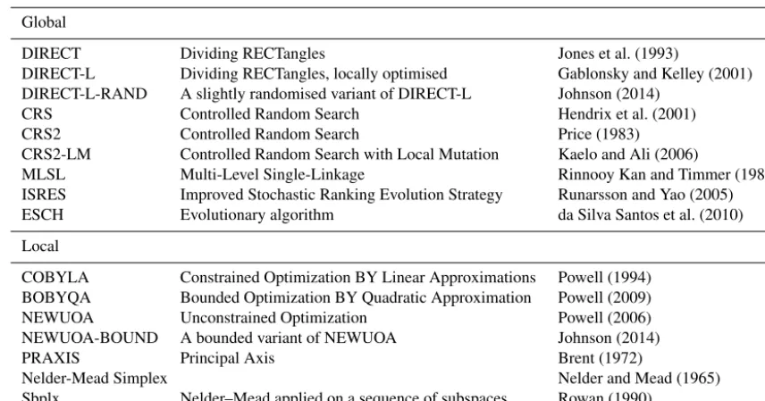
Table 1.Derivative-free optimisation algorithms from the NLopt toolbox supported in the Cyclops optimisation suite.
Global
DIRECT Dividing RECTangles Jones et al. (1993)
DIRECT-L Dividing RECTangles, locally optimised Gablonsky and Kelley (2001) DIRECT-L-RAND A slightly randomised variant of DIRECT-L Johnson (2014)
CRS Controlled Random Search Hendrix et al. (2001) CRS2 Controlled Random Search Price (1983) CRS2-LM Controlled Random Search with Local Mutation Kaelo and Ali (2006)
MLSL Multi-Level Single-Linkage Rinnooy Kan and Timmer (1987) ISRES Improved Stochastic Ranking Evolution Strategy Runarsson and Yao (2005) ESCH Evolutionary algorithm da Silva Santos et al. (2010)
Local
COBYLA Constrained Optimization BY Linear Approximations Powell (1994) BOBYQA Bounded Optimization BY Quadratic Approximation Powell (2009) NEWUOA Unconstrained Optimization Powell (2006) NEWUOA-BOUND A bounded variant of NEWUOA Johnson (2014) PRAXIS Principal Axis Brent (1972)
Nelder-Mead Simplex Nelder and Mead (1965) Sbplx Nelder–Mead applied on a sequence of subspaces Rowan (1990)
preprocessing of necessary model inputs (principally wind fields) and verification data (satellite altimeter data), running the wave model code, postprocessing of model outputs and generation of error statistics from comparisons of predicted and observed significant wave height fields.
Typically, date–time cycling is used to run a model at suc-cessive forecast cycles, or to break a long simulation into a succession of shorter blocks. The optimisation suite, on the other hand, uses integer cycling, with each cycle correspond-ing to a scorrespond-ingle evaluation of the objective function.
There are several tasks controlled by the optimisation suite. One of these is responsible for running an optimisa-tion algorithm to identify either an optimal parameter vec-tor from previous model runs or the next parameter vecvec-tor to be evaluated. This main optimisation task within the suite is implemented with Python code calling the NLopt Python toolbox (Johnson, 2014).
NLopt includes a selection of optimisation algorithms: both “local” solvers, which aim to find the nearest local min-imum to the starting point as efficiently as possible, and “global” solvers, which are designed to explore the full pa-rameter space, giving high confidence in finding the optimal solution out of a possible multitude of local minima. NLopt includes algorithms capable of using derivative information where available, which is not the case in our application, and Cyclops is restricted to the derivative-free algorithms listed in Table 1.
We have assumed that the sequence of parameter vectors tested by an optimisation algorithm is deterministic. Several of the algorithms available in NLopt have some inherently stochastic components. It is, however, possible to make these
algorithms “repeatably stochastic” by enforcing a fixed seed for the random number generator.
In NLopt, any combination of the following termination conditions can be set:
1. maximum number of iterations by each call of the opti-misation algorithm,
2. absolute change in the parameter values less than a pre-scribed minimum,
3. relative change in the parameter values less than a pre-scribed minimum,
4. absolute change in the function value less than a pre-scribed minimum,
5. relative change in the function value less than a pre-scribed minimum and
6. function value less than a prescribed minimum. In the second and third of these convergence criteria, the “change in parameter values” means the magnitude of the vector difference, i.e.
s Npar
P
n=1
(1xn)2.
to a file and returns an invalid1f value. Any of the termina-tion conditermina-tions listed above can be set by the user: the last of these can use a prescribed minimum f value as a con-vergence condition, while an invalidf value signals that the optimisation algorithm has stopped because a new parameter vectorxneeds to be evaluated externally by a model simula-tion. In this case, a file is written containing parameter names and values in a format that can be parsed by the modelling system to generate the needed input files for a simulation. At present, a generic namelist format is used as output from Cyclops for this purpose.
A “parameter definition” file is used to specify parameter names and their initial values, as used within the model. If a parameter is allowed to be adjusted by the optimisation suite, an allowable range is also set. This choice will generally re-quire some experience with the particular model. Within the optimisation suite, these adjustable parameters will be scaled linearly to normalised parameters x that lie between 0 and 1. Fixed parameters can be include for convenience, so that their names and values will be written to the namelist file but these are ignored by the optimisation suite.
The major tasks carried out by Cyclops on each cycle are 0. (first cycle only):Init: write initial normalised
parame-tersx0to file.
1. Optimise: run the optimisation code, starting fromx0
and evaluating every x in the sequence, until either a stopping criterion is met (in which case the task sends a “stop” message), or a parameter setxis reached that is not in the lookup table so needs evaluating (signalled by a “next” message).
2. Namelist: convertxto non-normalised parameters in a namelist file.
3. Model: create a new copy of the model suite, copy the namelist file to it and run it in non-daemon mode (i.e. so the task will not complete until the model suite shuts down). A new copy of the suite is made so that files created in one cycle do not overwrite those created on other cycles.
4. Table: read the resulting error value from the model suite and update the lookup table.
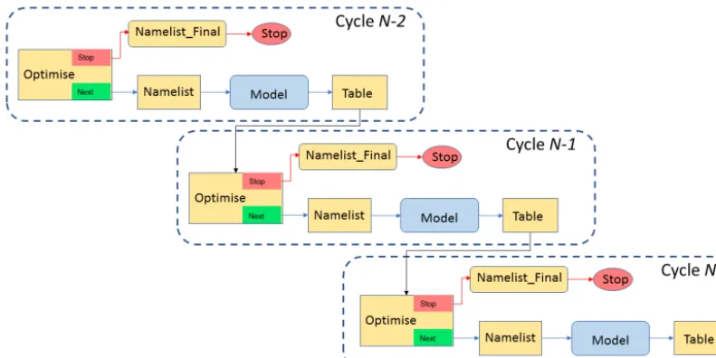
Within one cycle, the dependencies of the optimisation suite are simply
Optimise:next=>Namelist=>Model=>Table to make these tasks run sequentially when no stop condition
1At present,f <0 is treated as an “invalid” return value, which is appropriate for positive-definite error metrics, but the code could be modified to return the Python value “None” for invalidfin more general cases.
is met. We set a dependency on a previous cycle: Table[−P1]=>Optimise
(the notation −P1 denotes a negative displacement of one cycle period), to ensure that the lookup table is up to date with all previous results before starting the next opti-misation cycle and to prevent Cylc from running successive cycles concurrently. The stopping condition is handled by Optimise:stop=>Namelist_Final=>Stop
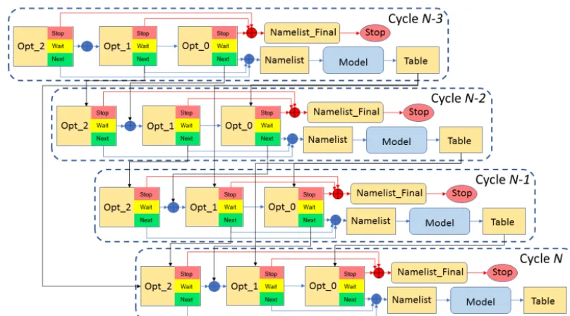
where the Namelist_Final task produces the final ver-sion of the namelist file, and the Stop task does a final wrap-up of the completed optimisation before the suite shuts down. For the purposes of good housekeeping, we can also add a Model_delete task to delete each copy of the model suite once all its outputs have been used. Also, tasks which will not be needed (e.g. “Namelist” if “Optimise” gives a “stop” message) can be removed, along with any dependencies on those tasks, by so-called “suicide triggers”. Figure 1 illustrates the workflow of the optimisation suite described above in graphical form.
The optimisation suite’s Model task for each cycle is a proxy for a copy of the full model suite being run for the corresponding parameter set. The model suite is run in non-daemon (non-detaching) mode, so that the Model task does not finish until the suite that it represents runs to completion. Information passed between the suites consists of two simple files: a “namelist” file containing parameter names and val-ues written by the optimisation suite for the model suite and an “error” file containing the single value of the error metric returned by the model suite.
Figure 1.Dependency graph for a version of the Cyclops optimisation suite in which no concurrent simulations are allowed, showing three successive cycles. Arrows represent dependency, in that a task at the head of an arrow depends on the task at the tail of the arrow meeting a specified condition (by default, this means completing successfully) before it can start.
2.3 Concurrent simulations
For some DFO algorithms, at least some parts of the se-quence of vectors tested are predetermined and independent of the function values found at those points. For example, BOBYQA (which we chose to use in the test application de-scribed below) sets up a quadratic approximation by sam-pling the initial point, plus a pair of points on either side of it in each dimension. With N parameters, the first 2N+1 iterations are spent evaluating these 2N+1 fixed points, re-gardless of the function values obtained there. In such situ-ations, the function values for each of these points could be evaluated simultaneously.
This can be done within Cylc by allowing tasks from mul-tiple cycles to run simultaneously. In practice, this means that multiple copies of the model suite are running simul-taneously, to the extent allowed by resource allocation on the host machine(s). This makes it imperative that a new copy of the model suite is made for each cycle.
If concurrent model simulations are allowed, this means that at any time there is a certain set of parameter vectors for which the function values are still being determined (we can call this the “active” set). We can add another parame-ter vector to that set if it will be selected by the optimisation algorithm regardless of the function values at the active pa-rameter vectors.
We would clearly like to determine that without needing specific knowledge of how the particular optimisation algo-rithm works. Instead, we use a simple empirical method. To this end, we supplement the lookup table (of vectors already computed, with the resultingf values) with a second table (the “active file”) listing the active vectors. We have the
func-tion evaluafunc-tion subroutine search forxfirst among the “com-pleted” vectors, then among the “active” vectors. If it findsx among the active vectors (for whichf is not yet known), it assignsf a random positive value (in this application, we do not re-initialise the random number generator with a fixed seed). Otherwise, it writesx to file and returns an “invalid” f value to force the optimisation algorithm to stop as usual.
The Python code controlling the optimisation algorithm has also been modified. Now, when the active file is empty, it will act as before, but if there are active vectors it will run a small set of repeated applications of the optimisation al-gorithm (Eq. 2), each of which will use a different set of randomisedf values for the active vectors. That is, in the Optimise task for cyclen+1, we evaluate
x(q)n+1=Opt
n
xm, fm(q) o
m=1,..., n
(6) for a set of iterationsq=1, . . ., Q, with
fm(q)=
fm completedm
random activem (7)
If these all result in the same choice ofxn+1to be
evalu-ated, a “next” message is sent to trigger further tasks for this cycle as before, since this choice is independent of the re-sults for the active parameter vectors. If not, we do not have a definitexn+1 to evaluate, and we must wait until at least
one of the presently active simulations has finished before trying again; a “wait” message is sent. But clearly this does not mean that the optimisation is complete.
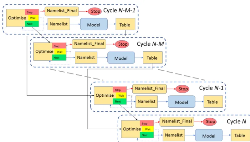
Figure 2.Dependency graph for an implementation of the Cyclops optimisation suite in which up toMconcurrent simulations are supported. Solid arrows represent dependency, in that a task at the head of an arrow depends on the task at the tail of the arrow meeting a specified condition (by default, this means completing successfully) before it can start. The dashed arrows represent a task retrying after a set interval. Only four cycles are shown, omitting tasks in intervening cycles and their dependencies.
Figure 3.Example of the cycling behaviour of an implementation of the Cyclops optimisation suite in which concurrent simulations are supported. Optimise tasks (purple boxes) which succeed trigger further tasks in the same cycle (blue boxes representing a sequence of Namelist, Model and Table tasks) and the Optimise task in the next cycle. Green arrows represent these dependencies on task suc-cess. Optimise tasks which fail to select a parameter vector indepen-dent of the result of active tasks retry (yellow arrows) at prescribed intervals until they succeed. The time axis is not to scale: Model tasks will typically have run times orders of magnitude longer than the run times of Optimise tasks. In this example, we suppose that the particular optimisation algorithm employed allows for up to five concurrent cycles during the initial stages.
started, concurrently with Model tasks already running for other cycles. They do not themselves need to run in parallel. We also need to consider how the Cylc suite dependency structure can accommodate concurrent simulations. This can be handled in two ways. In the first method, we let the Optimise task fail when it determines a “wait” condition, and utilise Cylc’s facility to retry failed tasks at specified intervals. We also replace the dependency
Table[−P1]=>Optimise with the combination
Optimise[−P1]=>Optimise Table[−PM]=>Optimise
where M is a specified maximum number of concur-rent simulations. This means that each cycle can first attempt to start a new model simulation as soon as the previous cycle’s simulation has started and theMth previous simulation has completed. The Optimise task will keep retrying at intervals until it is able to give either a “stop” or “next” signal. This method has a simple workflow structure, illustrated in Fig. 2, that does not change asMincreases.
vec-tor selected depends on all previous results (BOBYQA has this behaviour for a two-parameter optimisation). We also assume we have setM≥5. Hence, in cycle 2, the Optimise task’s randomised test shows that the same parameter vector will be chosen regardless of the outcome of the cycle 1 Model task, so that further cycle 2 tasks can start immediately. Sim-ilarly, the cycle 3 Model task does not need to wait for the active cycle 1 and 2 Model tasks to complete, and so forth up to cycle 5. But the cycle 6 Optimise task will detect that its choice of a parameter vector will depend on the results of the active Model tasks, so it will fail and retry. Under our as-sumptions it will not succeed until no other Model tasks are active, and this will remain the case for all subsequent cycles. The second method, described in Appendix A and used in the tests described here, uses more complex dependencies and additional Optimise tasks, instead of a single retrying Optimise task. It is somewhat more efficient in that there is no need to wait on a (short) retry interval before determining if a new cycle can start, but the workflow is more complicated and its complexity increases withM. Both methods achieve the same result; however, they both allow up to M model suites to run concurrently, rather than iterating through them in sequence.
It should be stressed that the optimisation code itself is simply run as a serial process in each case: it is simply re-quired to produce the single set of parameters, if any, for the next model run given the known results of the completed sim-ulations. As it checks that this parameter set is independent of the results of the presently active model runs without needing to know the actual results, no parallel processing is required within the optimisation code.
3 Application: a global wave hindcast based on ERA-Interim inputs
Here, we describe a global wave simulation, using the WAVEWATCH III model (WW3), forced by inputs from the ERA-Interim reanalysis (Dee et al., 2011), covering the pe-riod from January 1979 to December 2016. Such multi-year wave model simulations are a valuable means of obtaining wave climate information at spatial and temporal scales that are not generally available from direct measurements. It is rare for a particular location of interest to have a suitably long nearby in situ wave record, e.g. from a wave-recording buoy, to provide statistically reliable measures of climate variabil-ity on interannual timescales. And while satellite altimetry has provided near-global records of significant wave height that have been available for more than two decades, these have limited use for many climate applications for several reasons, including a return cycle that is too long to resolve typical weather cycles, limitations in providing nearshore measurements and lack of directional information. Model simulations can in many cases overcome these limitations,
but available measurements still play an essential role in cal-ibrating and verifying the simulations.
In our case, one of the principal motivations for carrying out this hindcast is to investigate the role of wave–ice interac-tions in the interannual variability of Antarctic sea ice extent, which plays an important role in the global climate system. The ERA-Interim reanalysis is a suitable basis for this work, providing a consistent long-term record, with careful con-trol on any extraneous factors (e.g. changing data sources or modelling methods) that might introduce artificial trends or biases into the records. While the ERA-Interim reanalysis in-cludes a coupled wave model, direct use of the wave outputs does not fully meet our requirements, which include the need for the wave hindcast to be independent of near-ice satellite waves, which were assimilated into the ERA-Interim reanal-ysis. Hence, we chose to carry out our own wave simulation, forced with ERA-Interim wind fields but with no assimila-tion of satellite wave measurements.
3.1 Comparison of model outputs with altimeter data Rather than being assimilated in the hindcast, satellite al-timetry measurements of significant wave height were used as an independent source of model calibration. These were obtained from the IFREMER database of multi-mission quality-controlled and buoy-calibrated swath records (Quef-feulou, 2004).
Swath records of significant wave height were first collo-cated to the hourly model outputs on the 1◦×1◦model grid. For each calendar month simulated, collocations were then accumulated in 3◦×3◦ blocks of nine neighbouring cells to produce error statistics, including model mean, altimeter mean, bias, root mean square error (RMSE) and correlation coefficientR. Spatial averages of these error statistics were taken over the full model domain between 65◦S and 65◦N (excluding polar regions with insufficient coverage).
The final error statistic used in the objective function was the spatially averaged RMSE, normalised by the spatially av-eraged altimeter mean, temporally avav-eraged over the simula-tion period, excluding spinup.
3.2 WW3 parameters
For this simulation, we used version 4.18 of the WW3 third-generation wave model (Tolman, 2014). The model repre-sents the sea state by the two-dimensional ocean wave spec-trum F (kxt ), which gives the energy density of the wave field as a function of wavenumberk, at each positionx in the model grid and timet of the simulation. The spectrum evolves subject to a radiative transfer equation,
∂N
∂t +∇x·(x˙N )+ ∂ ∂k
˙ kN+ ∂
∂θ ˙ θ N=S
σ, (8)
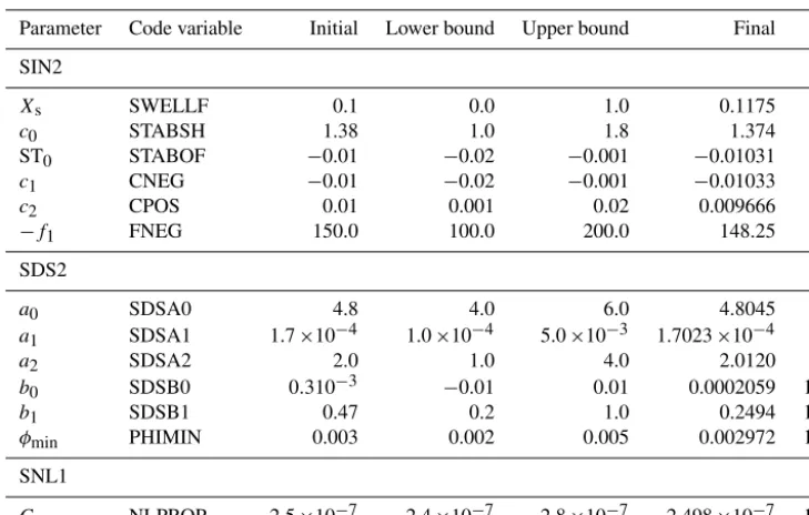
Table 2.Parameters used to calibrate the simulation using the source term package of Tolman and Chalikov (1996), for February through April 1997. The first two columns list the parameter as defined in the WW3 v4.18 user manual (Tolman, 2014) and as specified in WW3 namelist input. The namelist groupings correspond to parameterisations related to wind input (SIN2), dissipation (SDS2), nonlinear in-teractions (SNL1) and some “miscellaneous” parameters (MISC). Lower and upper bounds are specified for parameters adjusted during calibration, along with their final values, and the corresponding indexnof the normalised parameter vector, as used to label plots in Fig. 3. Other parameters were fixed at the initial value.
Parameter Code variable Initial Lower bound Upper bound Final n
SIN2
Xs SWELLF 0.1 0.0 1.0 0.1175 1
c0 STABSH 1.38 1.0 1.8 1.374 2
ST0 STABOF −0.01 −0.02 −0.001 −0.01031 3
c1 CNEG −0.01 −0.02 −0.001 −0.01033 4
c2 CPOS 0.01 0.001 0.02 0.009666 5 −f1 FNEG 150.0 100.0 200.0 148.25 6 SDS2
a0 SDSA0 4.8 4.0 6.0 4.8045 7
a1 SDSA1 1.7×10⁻⁴ 1.0×10⁻⁴ 5.0×10⁻³ 1.7023×10⁻⁴ 8
a2 SDSA2 2.0 1.0 4.0 2.0120 9
b0 SDSB0 0.310−3 −0.01 0.01 0.0002059 10
b1 SDSB1 0.47 0.2 1.0 0.2494 11
φmin PHIMIN 0.003 0.002 0.005 0.002972 12 SNL1
C NLPROP 2.5×10⁻⁷ 2.4×10⁻⁷ 2.8×10⁻⁷ 2.498×10⁻⁷ 13
propagation direction. The dots represent time derivatives. The terms on the left-hand side represent spatial advection and the shifts in wavenumber magnitude and direction due to refraction by currents and varying water depth. The source term Son the right-hand side represents all other processes that transfer energy to and from wave spectral components, including contributions from wind forcing, energy dissipa-tion and weakly nonlinear four-wave interacdissipa-tions.
Adjustable parameters within WW3 that can influence a deep-water global simulation such as the one described here are principally concentrated in the wind input and dissipa-tion source terms. It is generally necessary to treat these two terms together as a self-consistent “package” of input and dissipation treatments designed to work together. In this study, we undertook two separate calibration exercises, based on two “packages” of input/dissipation source terms: firstly, that of Tolman and Chalikov (1996) (activated in WW3 by the ST2 switch), and secondly, the Ardhuin et al. (2010) for-mulation (using the ST4 switch).
In Appendix B, we describe some of the details of these two packages. We also include some description of the WAM Cycle 4 (ST3) input source term formulation (Janssen, 1991), on which the ST4 input term is based, even though the ST3 package was not tested in this study.
In addition to the input and dissipation terms, the other main control on deep-water wave transformation is pro-vided by weakly nonlinear four-wave interactions
(Hassel-mann, 1962). Unfortunately, acceptable run time require-ments for multi-year simulations over extensive domains still preclude using a near-exact computation of these terms, such as the Webb–Resio–Tracy method (Webb, 1978; Tracy and Resio, 1982) that is available in spectral models including WW3 (van Vledder et al., 2000). Instead we use the much-simplified form of the discrete interaction approximation (Hasselmann et al., 1985), treating its proportionality con-stantCas a tunable parameter.
Common to both optimisations, sea ice obstruction was turned on (FLAGTR=4) with non-default values for the critical sea ice concentrations,c,0andc,n, between which wave obstruction by ice varies between zero and total block-ing: these were set to 0.25 and 0.75, respectively. All other available parameters beyond the input and dissipation terms were left with default settings, noting that shallow water pro-cesses, while activated, are not expected to have more than a negligible and localised influence on model outputs in a global simulation at 1◦resolution.
For initial testing, in which two sets (ST2 and ST4) of optimisation parameters were compared, we used a 1-month (January 1997) spinup to a 3-1-month calibration pe-riod (February–April 1997). The selection of the calibration period from the full extent of the satellite record was arbi-trary.
parame-Table 3.As for Table 2 but for parameters used to calibrate the simulation using the source term package of Ardhuin et al. (2010), for February through April 1997. The namelist groupings in bold correspond to parameterisations related to wind input (SIN4), dissipation (SDS4), nonlinear interactions (SNL1) and some “miscellaneous” parameters (MISC). Lower and upper bounds are specified for parameters adjusted during calibration, along with their final values, and the corresponding indexnof the normalised parameter vector, as used to label plots in Fig. 4.
Parameter Code variable Initial Lower bound Upper bound Final n
SIN4
βmax BETAMAX 1.52 1.0 2.0 1.5197 1
su TAUWSHELTER 1.0 0.0 1.5 0.9594 2
s2 SWELLF 0.8 0.5 1.2 0.8010 3
s1 SWELLF2 −0.018 −0.03 −0.01 −0.01812 4
s3 SWELLF3 0.015 0.01 0.02 0.01484 5
Rec SWELLF4 1.0×10⁵ 0.8×10⁵ 1.5×10⁵ 0.9973×10⁵ 6
s5 SWELLF5 1.2 0.8 1.6 1.2078 7
s7 SWELLF7 2.3×10⁵ 0.0 4.0×10⁵ 2.2600×10⁵ 8 SDS4
Cdssat SDSC2 −2.2×10⁻⁵ −2.5×10⁻⁵ 0.0 −2.1506×10⁻⁵ 9
Ccu SDSCUM −0.40344 −0.5 0.0 −0.4020 10
Cturb SDSC5 0.0 0.0 1.2 0.4168 11
δd SDSC6 0.3 0.0 1.0 0.2654 12
Br SDSBR 0.0009 0.0008 0.0010 0.0009035 13
CdsBCK SDSBCK 0.0 0.0 0.2 0.0 14
CdsHCK SDSHCK 0.0 0.0 2.0 0.0933 15
sB SDSCOS 2.0 0.0 2.0 2.0 16
SNL1
C NLPROP 2.5×10⁻⁷ 2.4×10⁻⁷ 2.8×10⁻⁷ 2.510×10⁻⁷ 17
ter names as defined (more completely than we do here) in the WW3 user manual (Tolman, 2014) and as specified in namelist inputs to the model. These tables include the ini-tial values of the parameters, the range over which they were allowed to vary and the final optimised values. Other param-eters not listed were kept fixed. A particular example was the input wind vertical levelzr(ST2)=zu(ST4)=10 m, which is a property of the input dataset and hence not appropriate to adjust. Others were left fixed after an initial test confirmed that they had negligible influence on the objective function, leaving 13 adjustable parameters for ST2 and 17 for ST4.
The selection of which parameters to tune, and the range over which they are allowed to vary, is an area where some (partly subjective) judgement is still required, based on some familiarity with the relevant model parameterisations. In this case, parameter ranges were chosen to be physically realistic and to cover the range of parameter choices used in previous studies reported in the literature.
3.3 Optimisation settings
We elected to primarily use the BOBYQA optimisation algo-rithm (Powell, 2009) for this study. Given that we expected WW3 to be already reasonably well-tuned for a global
sim-ulation such as our test case, we wished to use a local opti-misation algorithm that could reach a solution to a problem with 10–20 variables in as few iterations as possible. Of the algorithms available in NLopt that were included in the inter-comparison study of Rios and Sahinidis (2012), BOBYQA was found to be the most suitable in that respect. In particu-lar, it allows for concurrent model runs in the early stages of the optimisation process.
Both optimisations were stopped when either the abso-lute change in (normalised) parameter values was less than 0.0001, or the relative change in the objective function was less than 0.0001. Less stringent conditions were initially used, but the ability of the optimisation suite to be restarted with revised stopping criteria was invoked to extend the op-timisation.
model run times, especially as global methods do not gener-ally allow for parallel iterations.
A simpler approach is to still use a local algorithm but ini-tialise it at a range of different starting points. This was the approach we took for our next set of tests, restricted to the ST4 case, in which the initial value of each parameter was selected at random with uniform probability distribution over its allowed range. Five randomised tests were done, along with a control optimisation starting from the default param-eter set used previously. For these tests, we made some fur-ther simplifications in the interests of computational speed, running the hindcast for only 1 month (February 1997) and initialising all simulations from a common initial condition, spun up over 1 month with the default parameter set. Both simplifications detract from how applicable the resulting pa-rameter sets would be for hindcast applications but can be justified in allowing a more extensive examination of param-eter space with a given computational resource. A slightly re-duced set of ST4 parameters was optimised, omittingCdsBCK, CdsHCKandsB. The initial and final values of these parameters
from each of the tests are listed in Tables 4 and 5, respec-tively. The allowed range of each of the adjustable parame-ters was the same as in the previous simulations, as listed in Table 3, while both stopping criteria were relaxed to a value of 0.005.
Despite the expected high computational demands, we next attempted an optimisation using the global evolution-ary algorithm ESCH of da Silva Santos et al. (2010). This was initialised from the default parameter values and used the same 1-month hindcast, parameter ranges and stopping criteria as described above.
Following these test simulations, the ST4 parameterisa-tion was chosen for a final calibraparameterisa-tion, carried out over a 12-month period (January–December 1997) following a 1-month spinup (December 1996). This calibration was fi-nally terminated with both stopping criteria set to a value of 0.0001. This was a somewhat arbitrary choice made to observe the evolution of the solution. For practical applica-tions, the choice of stopping criteria should take into account the sensitivity of the objective function to measurement er-ror in the data used for the calibration, to avoid unnecessary “overtuning” of the model.
The full hindcast, from January 1979 to December 2016, was then run using the optimised parameter set. Compar-isons with altimeter data were made for each month from August 1991 onward.
Each WW3 simulation was run on 64 processors on a sin-gle core of either an IBM Power6 or a Cray XC50 machine. Other processing tasks within the suites were run on single processors. The resulting hindcast simulations required an average of approximately 25 min of wall-clock time to com-plete each month of simulation.
4 Results
4.1 Local optimisation of 3-month hindcasts with ST2 and ST4 source terms
The BOBYQA algorithm develops a quadratic model of the objective function. To do so, the first iteration evaluates the objective function at the initial point, then perturbs each com-ponent in turn by a positive increment, then by an equal neg-ative increment (leaving all other components at the initial value). This can be seen for the ST2 optimisation in Fig. 3, in which the bottom panel shows the sequence of (normalised) parameter values tested. With 13 adjustable parameters, this amounts to 27 iterations in this preliminary phase. As this sequence of parameter values is fixed, independent of the re-sulting objective function values, all of the first 27 iterations could have been run simultaneously as detailed above, if per-mitted by the queuing system. We, however, applied a limit of seven parallel iterations in line with anticipated resource limitations.
The 3-month ST2 optimisation only required a further seven iterations after this initial phase to reach a stopping cri-terion. The ST2 default parameter settings used as the start-ing point for optimisation resulted in an objective function value of 0.1901, which was reduced to 0.1424 in the optimi-sation process.
In the optimal configuration, none of the tunable parame-ters were at either of the limits of their imposed range, indi-cating that convergence to a true minimum (at least locally) had been reached. Most of the parameters were only slightly modified from their initial values: the largest changes were in parametersb0(reduced from 0.0003 to 0.0002059) andb1
(0.47 to 0.2493), both influencing the low frequency dissipa-tion term.
The ST4 3-month optimisation was initialised with the de-fault settings from the TEST451 case reported by Ardhuin et al. (2010), for which the objective function returned a value of 0.1427. Optimisation only managed to reduce this to 0.1419 (Fig. 4), indicating that the default ST4 parameter set was already quite closely tuned for our case, having been selected by Ardhuin et al. (2010) largely from broadly similar studies, i.e. global simulations (at 0.5◦resolution) compared with altimeter records.
Three of the parameters ended the optimisation at one end of their allowed range, in each case at the same value at which it was initialised. The 16th adjustable parameter (sB) controls the assumed directional spread of the
saturation-0 10 20 30 40 50 0
0.1 0.2 0.3 0.4 0.5 0.6 0.7 0.8 0.9 1
xn
Iteration
n=1 n=2 n=3 n=4 n=5 n=6 n=7 n=8 n=9 n=10 n=11 n=12 n=13
0 10 20 30 40 50
0.1 0.2 0.3 0.4 0.5
f(x)
(a)
(b)
Figure 4.Sequence of objective function values(a)and parameter vector components(b)at each iteration in the 3-month (February– April 1997) ST2 calibration. The red dashed line marks the optimal solution found.
based dissipation term by settingCdssat=0), whereas this term is turned off in the ST4 default; hence, both were initially set to zero. On the face of it, one might think that the op-timisation algorithm would have been free to explore solu-tions with positive values of these parameters, resulting in an optimal “hybrid” total dissipation term. In fact, the way the dissipation algorithm is coded, this form of the dissipa-tion term is not computed at all in the event thatCdsBCK=0.0, which would have been the case when the BOBYQA algo-rithm explored sensitivity toCdsHCKin the initial stages. This means that our choice of initial values may have spuriously caused the BOBYQA algorithm to underestimate sensitivity toCdsHCKand may have missed a distinct second local mini-mum (approximately corresponding to the parameter settings of Filipot and Ardhuin, 2012).
4.2 Tests with local optimisation with randomised initial parameter sets and global optimisation The next set of five tests compared results of the local BOBYQA algorithm starting from different parameter sets chosen at random within the allowed ranges (Table 4). The resulting final parameter sets, listed in Table 5, show that each test located a different minimum. This indicates that there are multiple local minima for the error metric in our chosen parameter ranges, in addition to the local minimum derived from the default parameters. The corresponding val-ues of the error metric were all slightly higher than the value (0.1454) obtained from the baseline optimisation starting from the default parameter set, although much reduced from their initial values (Table 4). Although none of those addi-tional local minima found so far have replaced the baseline set as a candidate for a global optimum, this gives no guar-antee that this would not be the case after a more thorough search.
The attempted global optimisation (using the ESCH algo-rithm) of the same hindcast had not converged to within the chosen tolerances after 800 cycles. However, in the course of its operation, it did identify over 30 parameter sets with slightly lower error metric than the minimum value (0.1450) obtained in the corresponding baseline local optimisation. The lowest value within 800 iterations was 0.1441, and the corresponding parameter values are included in Table 5. This supports our suspicion that a local optimisation algorithm cannot be relied upon to identify the global optimum for this hindcast problem. On the other hand, the very small decrease in the error metric obtained from this wider search does not give strong justification for making a significant change in parameters from near their default values. We need to bear in mind that the optimisation problem we have addressed in this set of tests (i.e. minimising RMS errors in significant wave height from a 1-month partial hindcast) is not quite the same as optimising this measure over a more representative period. 4.3 Local optimisation of 12-month hindcast with ST4
source terms
In the final 12-month ST4 optimisation, two additional pa-rameters were allowed to vary that were fixed in the 3-month optimisation, bringing the number of adjustable pa-rameters to 19. These were the critical sea ice concentration parametersc,0andc,nbetween which wave obstruction by ice varies between zero and total blocking: these had been fixed at 0.25 and 0.75, respectively, in the 3-month optimisa-tions. Otherwise, the initial parameters (Table 4) again corre-sponded to the ST4 defaults, which in this case produced an error metric of 0.1436. At the termination after 89 iterations (with the more stringent stopping criteria), this had decreased to 0.1431.
Table 4.Initial parameters used to calibrate the simulations using the source term package of Ardhuin et al. (2010), for February 1997, using randomised initial conditions (simulations 1–5). Simulation 0 is the control case, with default initial parameters.
Simulation number
Parameter Code variable 0 1 2 3 4 5
SIN4
βmax BETAMAX 1.520 1.215 1.160 1.538 1.660 1.550
su TAUWSHELTER 1.000 0.244 1.281 1.381 0.996 0.950
s2 SWELLF 0.800 0.962 0.948 0.582 0.995 1.026
s1 SWELLF2 −0.018 −0.022 −0.012 −0.026 −0.0253 −0.018 s3 SWELLF3 0.015 0.016 0.014 0.0116 0.0131 0.0159
Rec SWELLF4 1.000×10⁵ 1.428×10⁵ 1.368×10⁵ 1.295×10⁵ 0.837×10⁵ 0.809×10⁵
s5 SWELLF5 1.200 1.100 1.411 1.589 1.290 1.290
s7 SWELLF7 2.300×10⁵ 1.188×10⁵ 2.908×10⁵ 0.621×10⁵ 2.492×10⁵ 2.905×10⁵
SDS4
Csat
ds SDSC2 −2.200×10
−5 −1.528×10⁻⁵ −1.069×10⁻⁵ −1.493×10⁻⁵ −1.639×10⁻⁵ −1.303×10⁻⁵
Ccu SDSCUM −0.403 −0.159 −0.470 −0.488 −0.205 −0.387 Cturb SDSC5 0.000 1.116 1.074 1.025 0.476 0.882
δd SDSC6 0.300 0.957 0.596 0.947 0.855 0.583
Br SDSBR 9.00×10⁻⁴ 9.13×10⁻⁴ 8.24×10⁻⁴ 8.14×10⁻⁴ 9.73×10⁻⁴ 8.39×10⁻⁴
SNL1
C NLPROP 2.500×10⁷ 2.690×10⁷ 2.794×10⁷ 2.644×10⁷ 2.780×10⁷ 2.437×10⁷
Initial error score 0.1454 0.1685 0.2346 0.1722 0.2156 0.1677
Table 5. Final values of parameters from simulations using the source term package of Ardhuin et al. (2010), for February 1997, using BOBYQA with randomised initial conditions (simulations 1–5) and using ESCH with default initial parameters. Simulation 0 is the control case, using BOBYQA with default initial parameters.
Simulation number
Parameter Code variable 0 1 2 3 4 5 ESCH
SIN4
βmax BETAMAX 1.515 1.348 1.221 1.671 1.491 1.599 1.520
su TAUWSHELTER 0.950 0.244 1.275 1.385 1.035 0.953 0.898
s2 SWELLF 0.811 0.761 0.872 0.591 1.065 0.986 0.800
s1 SWELLF2 −0.0178 −0.0256 −0.0120 −0.0148 −0.0226 −0.0248 −0.018
s3 SWELLF3 0.0149 0.0168 0.0134 0.0112 0.0150 0.0170 0.0150
Rec SWELLF4 0.996×10⁵ 1.428×10⁵ 1.376×10⁵ 1.339×10⁵ 0.837×10⁵ 0.809×10⁵ 1.198×10⁵
s5 SWELLF5 1.201 1.099 1.406 1.589 1.291 1.290 0.973
s7 SWELLF7 2.30×10⁵ 1.19×10⁵ 2.84×10⁵ 0.64×10⁵ 2.47×10⁵ 2.89×10⁵ 2.42×10⁵
SDS4
Cdssat SDSC2 −2.12×10⁻⁵ −1.75×10⁻⁵ −0.09×10⁻⁵ −1.93×10⁻⁵ −2.05×10⁻⁵ −1.29×10⁻⁵ −2.34×10⁻⁵
Ccu SDSCUM −0.401 −0.158 −0.469 −0.488 −0.209 −0.387 −0.454
Cturb SDSC5 0.386 1.116 1.067 1.027 0.526 0.831 0.567
δd SDSC6 0.246 0.957 0.560 0.940 0.860 0.585 0.043
Br SDSBR 9.03×10⁻⁴ 9.19×10⁻⁴ 8.26×10⁻⁴ 8.20×10⁻⁴ 9.72×10⁻⁴ 8.38×10⁻⁴ 9.09×10⁻⁴
SNL1
C NLPROP 2.51×10⁷ 2.69×10⁷ 2.80×10⁷ 2.69×10⁷ 2.78×10⁷ 2.44×10⁷ 2.45×10⁷
Error score 0.1450 0.1479 0.1513 0.1515 0.1501 0.1500 0.1441
Iterations 38 37 41 62 37 39 800+
0 10 20 30 40 50 0 0.1 0.2 0.3 0.4 0.5 0.6 0.7 0.8 0.9 1 xn Iteration n=1 n=2 n=3 n=4 n=5 n=6 n=7 n=8 n=9 n=10 n=11 n=12 n=13 n=14 n=15 n=16 n=17
0 10 20 30 40 50
0.15 0.16 0.17 0.18 f(x) (a) (b)
Figure 5.Sequence of objective function values(a)and parameter vector components(b)at each iteration in the 3-month (February– April 1997) ST4 calibration. The red dashed line marks the optimal solution found.
(Table 3). An exception was the 11th adjustable parame-ter,Cturb, scaling the strength of the turbulent contribution
to dissipation, which finished the 3-month optimisation at 0.41298, but at 0.0 (the lower bound) in the 12-month simu-lations.
For this longer optimisation, we have additionally com-puted a measure of the sensitivity of the objective function, using the initial phase of the BOBYQA iterations to estimate the change in the (un-normalised) parameter required to pro-duce a 0.1 % change in the objective function. This is listed as “delta” in the seventh column of Table 6, and provides a measure, at least in relative terms, of the bounds within which each parameter value has been determined.
The full hindcast, run from 1979 to 2016, could be com-pared with satellite data from August 1991 onward. The re-sulting bias in significant wave height, averaged over the Au-gust 1991–December 2016 comparison period, is shown in Fig. 6. Positive biases are obtained in latitudes south of 45◦S, particularly south of Australia and in the South Atlantic. This is also seen in the vicinity of some island groups (notably French Polynesia, Micronesia, the Maldives, Aleutians, Car-ribean and Azores), which may be indicative of insufficient
−0.4−0.35−0.3−0.25−0.2−0.15−0.1−0.05 0 0.05 0.1 0.15 0.2 0.25 0.3 0.35 0.4 Significant w ave height bias (m)
−0.2 −0.2 −0.2 −0.2 −0.2 −0.2 −0.2 −0.2 −0.2 −0.2 0 0 0 0 0 0 0 0 0 0 0 0 0 0 0 0 0 0 0 0 0 0 0 0 0 0 0 0 0 0 0 0 0 0 0 0 0 0 0
0 00
0 0 0 0 0 0 0 0 0 0 0 0 0 0 0 0 0 0 0 0 0 0 0.2 0.2 0.2 0.2 0.2 0.2 0.2 0.2 0.2 0.2 0.2
0.2 0.2 0.2 0.2
0.2 0.2
0.2
0.4 0.4
0 30 60 90 120 150 180 210 240 270 300 330 360
−90 −75 −60 −45 −30 −15 0 15 30 45 60 75 90
Figure 6.Bias in significant wave height from the hindcast com-pared with satellite altimeter measurements, over the period Au-gust 1991–December 2016.
subgrid-scale obstruction. On the other hand, negative biases are seen near the western sides of major ocean basins and in the “swell shadow” to the northeast of New Zealand. A similar pattern is seen in the results reported by Ardhuin et al. (2010) for their TEST441 case (their Fig. 9).
Normalised root mean square error (i.e. RMSE divided by the observed mean) from the same comparison, again aver-aged over the period August 1991–December 2016, is shown in Fig. 7. Note that the objective function for our optimisa-tion used this measure, spatially averaged over ocean waters between 61◦S and 61◦N. For the majority of the ocean
sur-face, this lies in the range 0.08–0.14 but with higher values near some island chains and the western boundaries of ocean basins. Again, similar results were reported by Ardhuin et al. (2010).
5 Discussion
cli-Table 6.As for Table 3 but for parameters used to calibrate the simulation using the source term package of Ardhuin et al. (2010), for January– December 1997. The delta value in the seventh column is the estimated change in the (un-normalised) parameter required to produce a 0.1 % change in the objective function.
Parameter Code variable Initial Lower bound Upper bound Final Delta n
SIN4
βmax BETAMAX 1.52 1.0 2.0 1.5194 0.02498 1
su TAUWSHELTER 1.0 0.0 1.5 0.9339 0.2706 2
s2 SWELLF 0.8 0.5 1.2 0.8224 0.0206 3
s1 SWELLF2 −0.018 −0.03 −0.01 −0.01721 0.00064 4
s3 SWELLF3 0.015 0.01 0.02 0.01526 0.00042 5
Rec SWELLF4 1.0×10⁵ 0.8×10⁵ 1.5×10⁵ 0.9888×10⁵ 0.2328×10⁵ 6
s5 SWELLF5 1.2 0.8 1.6 0.9360 0.3974 7
s7 SWELLF7 2.3×10⁵ 0.0 4.0×10⁵ 2.2433×10⁵ 0.7911×10⁵ 8 SDS4
Cdssat SDSC2 −2.2×10⁻⁵ −2.5×10⁻⁵ 0.0 −2.1433×10⁻⁵ 0.0087×10⁻⁵ 9
Ccu SDSCUM −0.40344 −0.5 0.0 −0.40194 0.02145 10
Cturb SDSC5 0.0 0.0 1.2 0.0 – 11
δd SDSC6 0.3 0.0 1.0 0.2736 0.0928 12
Br SDSBR 9.0×10⁻⁴ 8.0×10⁻⁴ 10.0×10⁻⁴ 8.9788×10⁻⁴ 0.0951 ×10⁻⁴ 13
CdsBCK SDSBCK 0.0 0.0 0.2 0.0 – 14
CdsHCK SDSHCK 0.0 0.0 2.0 0.0 – 15
sB SDSCOS 2.0 0.0 2.0 2.0 0.0757 16
SNL1
C NLPROP 2.5×10⁷ 2.4×10⁷ 2.8×10⁷ 2.5181×10⁷ 0.1191×10⁷ 17 MISC
c,0 CICE0 0.25 0.15 0.45 0.2413 0.1285 18
c,n CICEN 0.75 0.55 0.85 0.7521 0.2358 19
0 0.02 0.04 0.06 0.08 0.1 0.12 0.14 0.16 0.18 0.2 0.22 0.24 0.26 0.28 0.3 Significant wave height normalised RMSE
0.1 0.1 0.1
0.1
0.1
0.1 0.1
0.1
0.1
0.1
0.1 0.1
0.1
0.2
0.2 0.2
0.2
0.2
0.2
0.2
0.2
0.2 0.2
0.2 0.2
0.2
0.2 0.2
0.2
0.2 0.2
0.2 0.2 0.3 0.3
0.3
0.3 0.3
0.3
0.3 0.3
0 30 60 90 120 150 180 210 240 270 300 330 360
−90 −75 −60 −45 −30 −15 0 15 30 45 60 75 90
Figure 7.Normalised root mean square error in significant wave height from the hindcast compared with satellite altimeter measure-ments, over the period August 1991–December 2016.
mate modelling systems, to optimise the parameters of such a system under its control, in a way that is simple to implement and flexible in choice of optimisation algorithm.
We have shown this to be a practical method for optimising 10–20 parameters in a model application of sufficient com-plexity to require several hours per simulation in a parallel processing computing environment. For applications that are yet more time-consuming, it is becoming increasingly com-mon (Bellprat et al., 2012; Wang et al., 2014; Duan et al., 2017) to first build a surrogate model to provide a statisti-cal emulator for the actual model and then apply an opti-misation algorithm to the surrogate model. Such multi-stage model optimisation frameworks are beyond the scope of this paper, but the flexibility of our approach could potentially bring benefits to them as well. For example, it may be worth considering a hybrid approach of using a surrogate model to quantify the role of the full set of model parameters and perform an initial global optimisation, before switching to a method such as ours for a final refinement using the original model directly.
results suggest the need in some circumstances to apply a more global method. This is not difficult to do in principle, with multiple algorithms, both global and local, implemented in Cyclops. However, the generally higher computational de-mands of a global algorithm put a limit on such applications. In this study, we have only been able to undertake a prelim-inary exploration of the wider parameter space of our single chosen test case. This did, however, illustrate that the pos-sibility of multiple alternative local minima must be consid-ered.
As we have seen, there remains a need for care with the choices of which parameters to attempt to optimise and what bounds to set on their values. Most optimisation algorithms are intended for continuously variable parameters and may rely on the objective function having a continuous depen-dence on these parameters. In many cases, it is clear which parameters fall into this category, as opposed to discrete val-ued options. But in some cases, model code may make bi-nary choices based on real parameters lying within discrete ranges, which may break this assumption. Hence, the Cy-clops optimisation suite is best employed in conjunction with a good understanding of the role each parameter plays in the model and the interplay between them.
It is also important to be aware of the role played by the de-sign of the error metric, which may make it sensitive to some parameters and insensitive to others. One should be wary of accepting a large change in these insensitive parameters to achieve a tiny improvement in the chosen error metric, when the resulting model could then perform poorly against other relevant criteria. In the particular wave modelling case we have investigated, our approach would not be sufficient on its own to identify suitable values of the large set of WW3 parameters without guidance from previous studies.
Tett et al. (2017) point out that the inherently chaotic na-ture of the climate system means that a certain level of noise is introduced into evaluations of an atmospheric model sim-ulation, which can cause problems in evaluating the termi-nation criteria. They describe a procedure to rerun a simula-tion that had nominally satisfied the prescribed convergence criteria, with randomised perturbations before determining whether or not to terminate. Unlike the atmosphere, ocean surface waves are an essentially dissipative system, and per-turbations introduced in the initial conditions and forcing will tend to diminish, rather than grow, with time. As a result, noise in the objective function was not so relevant for our wave hindcast application as for atmospheric models but may need to be addressed in systems with an underlying chaotic nature, possibly through implementing similar measures to those of Tett et al. (2017) into Cyclops.
Similarly, the dissipative nature of ocean waves means that a cost function based on a spatial average of the (temporal) RMSE of model–data comparisons will not be subject to the level of chaotic variability seen in similar measures for atmo-spheric models. Small-scale variability in wave model output is therefore more likely to be genuinely sensitive to
parame-ter variation. In that case, it is worth capturing such variabil-ity in the cost function, whereas for a chaotic system it may be wiser to average out such variability before evaluating the cost function.
6 Conclusions
The Cyclops Cylc-based optimisation suite offers a flexi-ble tool for tuning the parameters of any modelling system that has been implemented to run under the Cylc workflow engine. Minimal customisation of the modelling system is required beyond providing tasks to input and apply model parameter values in a simple namelist format and output the value of the scalar error metric that is to be minimised. This then allows any of 16 optimisation algorithms (from the NLopt toolbox) to be applied to the optimisation. This opti-misation suite is expected to be especially applicable to oper-ational forecasting systems, where minimal reconfiguration is required between “tuning” and “operational/production” versions of the forecast suite.
Results of the initial test case we have investigated, a global hindcast using a spectral wave model forced by ERA-Interim input fields, illustrate that the method is applicable to a modelling system of moderate complexity, both in terms of the number of parameters to tune and the computational resources required, at least for the purposes of local optimi-sation to fine tune a model that already has a more-or-less well-developed initial parameter set from previous studies. Investigations of systems that require a more global tuning approach, or are more computationally demanding, remain for future work.
Code and data availability. Cyclops-v1.0 has been published through Zenodo (https://doi.org/10.5281/zenodo.837907) under a Creative Commons Attribution Share-Alike 4.0 licence.
Cylc is available from GitHub (https://cylc.github.io/cylc/) and Zenodo (https://zenodo.org/badge/latestdoi/1836229) under the GPLv3 licence.
The following additional software and data was used in this study:
– NLopt nonlinear-optimization package (version 2.4.2) (http://ab-initio.mit.edu/nlopt, Johnson, 2014),
– Wavewatch III (version 4.18) (http://polar.ncep.noaa.gov/ waves/wavewatch/),
– ERA-Interim surface fields (https://www.ecmwf.int/en/ forecasts/datasets/archive-datasets/reanalysis-datasets/ era-interim),
Appendix A: Handling concurrent simulations through dependencies
An alternative way to allow for concurrent simulations involves modifying the simple Cylc suite described above to have several versions of the “Optimise” task. Now “Opt_m” runs the optimisation algorithm when there are m active model simulations still running, with mranging from 0 to a set maximum M−1, where M is the maximum number of concurrent cycles we chose to allow. There is a more complex set of dependencies to ensure that this is the case. In particular, there is a condition
Table[−P(m+1)]=>Opt_m
to ensure that the lookup table has been updated with the results of all completed (i.e. inactive) cycles. If that is the case, the optimisation code will be run to determine if a new model simulation can be launched while those mtasks are active. If not, the suite will wait until one of the active model runs completes and try again with “Opt_m−1” and so forth. The dependency diagram for the case in which up to three concurrent simulations are allowed (i.e.M=3) is illustrated in Fig. A1. Assume, for example, that we are still well short of convergence and that the optimisation algorithm is such that the next parameter set tested depends on all previous re-sults. Then, “Opt_2” and “Opt_1” will always give a “wait” message, and “Opt_0” will be needed on each cycle. This ef-fectively produces the same behaviour as in Fig. 1, with each cycle waiting for the immediately preceding cycle to com-plete before “Opt_0” can start, leading to a new model run. If, on the other hand, the algorithm never depends on the re-sults of the previous two (active) calculations, “Opt_2” will always give a “next” message. This removes the “Opt_1 and “Opt_0” tasks (and any dependencies upon them), leading to the “Model” task being called for cycleNas soon as the cy-cleN−3 model run has completed and updated the lookup table, even if the cycleN−2 andN−1 “Model” tasks are still running.
Appendix B: WW3 source term parameterisations B1 Tolman and Chalikov input+dissipation source
term package
The input source term is defined as
Sin(kθ )=σβN (kθ ), (B1)
whereβis a non-dimensional wind–wave interaction param-eter, which has a parameterised dependence on wind speed and direction, through boundary layer properties influenced by the wave spectrum. These dependencies are, however, fully determined with no user-adjustable terms, so we omit the details here.
This input term was, however, adjusted by Tolman (2002) following a global test case to ameliorate an excessive dissi-pation of swell in weak or opposing winds, in which casesβ can be negative. This is done by applying, whenβis negative, a swell filtering scaling factor with a constant valueXs for
frequencies below 0.6fp (where fpis the peak frequency),
scaling linearly up to 1 at 0.8fp, with higher frequencies
un-modified.
The same study also led to the introduction of a correction for the effects of atmospheric stability on wave growth iden-tified by Kahma and Calkoen (1992) by replacing the wind speeduwith an effective wind speedue, with
ue
u
2
=1+c1tanh(max(0, f1{ST−ST0})) (B2)
+c2tanh
max
0, f1
c1
c2
{ST−ST0}
,
where ST is a bulk stability parameter, ST=hg
u2h Ta−Ts
T0
, (B3)
in terms of air, sea and reference temperatures Ta,Ts and
T0, respectively, anduhis the wind speed at reference height h=10 m, withg the gravitational acceleration. As air and sea surface temperature fields are available from the ERA-Interim dataset, it was possible to apply this parametrisation, treatingc0,c1,c2,f1 and ST0 as adjustable dimensionless
parameters.
The dissipation term consists of a dominant low-frequency constituent, with an empirical frequency dependence param-eterised by constantsb0,b1,φminand a high-frequency term,
parameterised by constantsa0,a1anda2, the details of which
we leave for the WW3 manual (Tolman, 2014) and original references therein.
B2 WAM Cycle 4 source term package
The input source term implemented in WAM Cycle 4 by Janssen (1982) was based on the wave growth theory of Miles (1957). The starting point is the assumption the wind speedU has a logarithmic profile, so that if the wind fields input to the model are specified at elevationzu, then
U (zu)= u∗
κ log
z u z1
, (B4)
whereu∗ is the friction velocity, defined by the total wind
stressτ =u2∗,κis von Karman’s constant, andz1is a
rough-ness length modified by wave conditions: z1=
z0
√
1−τw/τ
, (B5)
in whichτw is the magnitude of the wave-supported stress,
while
Figure A1.Dependency graph for the Cyclops optimisation suite, configured to use dependencies to allow for concurrent simulations. This example shows four successive cycles, for the case in which up to three parallel simulations are allowed. Arrows represent dependency, which in some cases are combined by a logical OR (enclosed “+” symbol). All tasks and explicit dependencies (other than suicide triggers) are shown for cycleN, but dependencies on cycles beforeN−3 are omitted for clarity.
withα0a tunable dimensionless parameter.
The wave-supported stress can be equated to the rate of momentum transfer between wind and waves:
τw= Z
dkdθk
CSin(kθ ), (B7)
wherecis the wave phase velocity. The WAM Cycle 4 input source term is then given by
Sin(k, θ )=
ρa
ρw
βmax
κ2 e
ZZ4u∗
C +zα
2
(B8) [max(cos(θ−θu) ,0)]pinσ N (k, θ )+Sout(kθ ),
with
Z=log(kz1)+
κ
cos(θ−θu) uC∗+zα
. (B9)
In these terms,ρaandρware the densities of air and water,
βmax is a dimensionless constant, zα is a wave-age tuning parameter, andpinis a parameter controlling the directional
dependence relative to the wind directionθu.
The interdependence ofτwandSinexpressed in Eqs. (B7)
and (B8) creates an implicit functional dependence ofu∗on
U andτw/τ. In practice, this dependence can be tabulated,
using the resolved model spectrum for the low-frequency (k < kmax)part of Eq. (B7), above which af−5diagnostic
tail is assumed.
TheSoutterm represents a linear damping of swells, in the
form (Bidlot, 2012)
Sout(k, θ )= (B10)
2s1κ
ρa
ρw u∗
C
2
cos(θ−θu)− κC u∗log(kz
0)
σ N (k, θ ) ,
withs1set to 1 (0) to turn on (off) the damping.
Dissipation is represented in the form
Sds(k, θ )=Cdsα2σ "
δ1
k k
+δ2 k
k
2#
N (k, θ ) , (B11)
whereCds is a dimensionless constant, and δ1 and δ2 are
weighting parameters. These take valuesCds= −1.33,δ1=
0.5 and δ2=0.5 in the ECMWF implementation of WAM
as reported by Bidlot (2012) but are adjustable within WW3. Mean wavelength and frequency are defined as
k=
RkpN (k, θ )dk R
N (k, θ )dk 1/p
, (B12)
and σ=
RσpN (k, θ )dk R
N (k, θ )dk 1/p
, (B13)
withp=0.5 andp=1 being the respective WAM defaults (Bidlot, 2012), while mean steepness is