https://doi.org/10.5194/gmd-11-2739-2018 © Author(s) 2018. This work is distributed under the Creative Commons Attribution 4.0 License.
MOPSMAP v1.0: a versatile tool for the modeling of
aerosol optical properties
Josef Gasteiger1and Matthias Wiegner2
1Faculty of Physics, University of Vienna, Vienna, Austria
2Meteorologisches Institut, Ludwig-Maximilians-Universität, Munich, Germany
Correspondence:Josef Gasteiger ([email protected]) Received: 23 February 2018 – Discussion started: 29 March 2018
Revised: 17 June 2018 – Accepted: 29 June 2018 – Published: 11 July 2018
Abstract.The spatiotemporal distribution and characteriza-tion of aerosol particles are usually determined by remote-sensing and optical in situ measurements. These measure-ments are indirect with respect to microphysical properties, and thus inversion techniques are required to determine the aerosol microphysics. Scattering theory provides the link be-tween microphysical and optical properties; it is not only needed for such inversions but also for radiative budget cal-culations and climate modeling. However, optical modeling can be very time-consuming, in particular if nonspherical particles or complex ensembles are involved.
In this paper we present the MOPSMAP package (Mod-eled optical properties of ensembles of aerosol particles), which is computationally fast for optical modeling even in the case of complex aerosols. The package consists of a data set of pre-calculated optical properties of single aerosol par-ticles, a Fortran program to calculate the properties of user-defined aerosol ensembles, and a user-friendly web inter-face for online calculations. Spheres, spheroids, and a small set of irregular particle shapes are considered over a wide range of sizes and refractive indices. MOPSMAP provides the fundamental optical properties assuming random particle orientation, including the scattering matrix for the selected wavelengths. Moreover, the output includes tables of fre-quently used properties such as the single-scattering albedo, the asymmetry parameter, or the lidar ratio. To demonstrate the wide range of possible MOPSMAP applications, a selec-tion of examples is presented, e.g., dealing with hygroscopic growth, mixtures of absorbing and non-absorbing particles, the relevance of the size equivalence in the case of nonspheri-cal particles, and the variability in volcanic ash microphysics.
The web interface is designed to be intuitive for expert and nonexpert users. To support users a large set of default settings is available, e.g., several wavelength-dependent re-fractive indices, climatologically representative size distribu-tions, and a parameterization of hygroscopic growth. Calcu-lations are possible for single wavelengths or user-defined sets (e.g., of specific remote-sensing application). For ex-pert users more options for the microphysics are available. Plots for immediate visualization of the results are shown. The complete output can be downloaded for further applica-tions. All input parameters and results are stored in the user’s personal folder so that calculations can easily be reproduced. The web interface is provided at https://mopsmap.net (last access: 9 July 2018) and the Fortran program including the data set is freely available for offline calculations, e.g., when large numbers of different runs for sensitivity studies are to be made.
1 Introduction
Optical modeling codes
(+wrapper codes)
Data set of optical properties of single particles
(netcdf files)
Mie (Mishchenko)
T-matrix method (Mishchenko) IGOM (Yang)
ADDA (Yurkin)
Fortran program for interpolation and ensemble averaging
Input file (microphysics, wavelengths, etc)
Optical properties of particle ensemble
Sect. 2.2
Sect. 2.3
Sect. 3
User manual
Web interface
Sect. 4
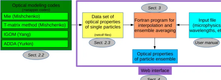
Figure 1.Scheme of the MOPSMAP package, including the optical modeling codes applied to create the data set.
to predict the influence of particles on the state of the atmo-sphere; see, e.g., Baklanov et al. (2014).
Aerosol properties and distributions are often quantified by ground-based and spaceborne optical remote sensing and by optical in situ measurements. These measurements are indirect with respect to microphysical properties (e.g., par-ticle size) because they measure optical quantities and re-quire the application of inversion techniques to retrieve mi-crophysical properties. Precise knowledge on the link be-tween microphysical and optical properties is needed for the inversion. This link is provided by optical modeling, i.e., the optical properties of particles are calculated based on their microphysical properties. Optical modeling is required also for other applications, e.g., for radiative transfer, numerical weather prediction, and climate modeling. As optical mod-eling can be very time-consuming, it is often inevitable to pre-calculate optical properties of particles and store them in a lookup table, which is then accessed by the inversion pro-cedures or subsequent models.
In our contribution we describe the MOPSMAP (Mod-eled optical properties of ensembles of aerosol particles) package, which consists of a data set of pre-calculated op-tical properties of single aerosol particles, a Fortran program which calculates the properties of user-defined aerosol en-sembles from this data set, and a user-friendly web inter-face for online calculations. Figure 1 illustrates the overall scheme of the package, including the optical modeling codes (green box) needed once to prepare the underlying data set. MOPSMAP is either provided via an interactive web inter-face at https://mopsmap.net or via download as an offline application. The former is possible as MOPSMAP is com-putational very efficient. Compared to other data sets with predefined aerosol components, such as OPAC (Hess et al., 1998), compared to existing online Mie tools such as the one provided by Prahl (2018), and compared to GUI tools such as MiePlot Laven (2018), MOPSMAP is more flexible with respect to the characteristics of the aerosol ensembles. More-over, our data set considers not only spherical particles but also spheroids and a small set of irregularly shaped dust
parti-cles. The output includes ASCII tables for further evaluation, netCDF files for direct application in the radiative transfer model uvspec (Emde et al., 2016), and plots, e.g., for educa-tional purposes.
In Sect. 2, after defining aerosol properties, we describe how existing optical modeling codes were applied (green box in Fig. 1) to create the optical data set of single parti-cles (yellow box). Subsequently, in Sect. 3, we describe the Fortran program (orange box) that uses this data set to cal-culate optical properties of user-defined particle ensembles. The web interface for online application of the MOPSMAP package is introduced in Sect. 4. To demonstrate the potential of MOPSMAP, several applications are discussed in Sect. 5 before we sum up our paper and give an outlook.
2 Background and the MOPSMAP data set
The optical properties of a particle with known microphys-ical properties are calculated by optmicrophys-ical modeling. For the creation of the basic data set of MOPSMAP, optical model-ing of smodel-ingle particles has been performed. In this section, we first define microphysical and optical properties of single particles and then describe how we created the data set using existing optical modeling codes.
We emphasize that the data set is, in principle, applicable to the complete electromagnetic spectrum; however, we use, for simplicity, the term “light” and consequently “optics” in-stead of more general terms.
2.1 Definition of particle properties
The description of particle properties is well-established and can be found in textbooks with varying levels of detail. Thus, we can restrict ourselves to a brief summary of those proper-ties that are of special relevance for MOPSMAP.
The microphysical properties of an aerosol particle are de-scribed by its shape, size, and chemical composition.
with a large variety of different shapes. Mineral dust (e.g., Kandler et al., 2009) and volcanic ash aerosols (e.g., Schumann et al., 2011b) are important examples of the latter, but, for example, pollen, dry sea salt or soot par-ticles are also usually nonspherical. A quite common ap-proach to consider the particle shape is the approximation us-ing spheroids or distributions of spheroids (Hill et al., 1984; Mishchenko et al., 1997; Kahn et al., 1997; Dubovik et al., 2006; Wiegner et al., 2009). Spheroids originate from the rotation of ellipses about one of their axes. Only one pa-rameter is required for the shape description. Mishchenko and Travis (1998) use the “axial ratio”m, which is the ra-tio between the length of the axis perpendicular to the ro-tational axis and the length of the roro-tational axis. By con-trast, Dubovik et al. (2006) use the “axis ratio”d, defined as the inverse ofm. Spheroids withm<1,d>1 are called prolate (elongated) whereas spheroids with m>1, d<1 are oblate (flat) spheroids. The aspect ratio0is the ratio be-tween the longest and the shortest axis, i.e.,0= 1
m =din the case of prolate spheroids and0=m=d1 in the case of oblate spheroids. Spheroids with0=1 are spheres.
The size of a particle is commonly described by its ra-dius or diameter. While this is unambiguous in the case of spheres, more detailed specifications are necessary for any kind of nonspherical particles. Often the size of an equivalent sphere is used for the description of the nonspherical parti-cle size: the volume-equivalent radius rvof a particle with
known volumeV (containing the particle mass, i.e., without cavities) is
rv=
3
r
3V
4π, (1)
whereas the cross-section-equivalent radius rc of a
parti-cle with known orientation-averaged geometric cross section Cgeois
rc= r
Cgeo
π . (2)
In the case of spheroids,rcis equal to the radius of a sphere
having the same surface area (as used by Mishchenko and Travis, 1998). For the conversion betweenrvandrc, the
ra-dius conversion factor
ξvc=
rv
rc
= 3
s
3√π 4
V
Cgeo3/2
(3)
is used (Gasteiger et al., 2011b).ξvcis equal to 1 in the case
of spheres and decreases with increasing deviation from a spherical shape. Another definition of size is given by the radius of a sphere that has the same ratio between volume and geometric cross section as the particle
rvcr=
3V 4Cgeo
=ξvc3rc. (4)
This definition corresponds to the case “VSEQU” presented by Otto et al. (2011), to the “effective radius” in Eq. (5) of Schumann et al. (2011a), and is more sensitive to non-sphericity than rv or rc. For example, a particle with rc=
1 µm and ξvc=0.9 implies that rv=0.9 µm and rvcr=
0.729 µm.
For setting up a data set of optical properties for different wavelengths, it is highly beneficial to make use of the size parameter
x=2π r
λ . (5)
The size parameterxdescribes the particle size relative to the wavelengthλ. The advantage of usingxis that optical prop-erties (qext, ω0, andF, as defined below) at a given
wave-length are fully determined by its shape, refractive indexm, andx. Equivalent size parametersxv,xc, andxvcrare
calcu-lated from the equivalent radii, analogously to Eq. (5). The chemical composition of a particle determines its complex wavelength-dependent refractive index m. The imaginary partmiis relevant for the absorption of light inside
the particle, whereby an imaginary part of zero corresponds to non-absorbing particles.
The optical properties of a nonspherical particle depend on the orientation of the particle relative to the incident light. In our data set we assume that particles are oriented randomly; thus, the optical properties are stored as orientation averages (Mishchenko and Yurkin, 2017).
The orientation-averaged optical properties at a given wavelength are fully described by the extinction cross sec-tionCext, the single-scattering albedoω0and the scattering
matrix F(θ ), where θ is the angle by which the incoming light is deflected during the scattering process (“scattering angle”). The extinction cross sectionCextcan be normalized
by the orientation-averaged geometric cross sectionCgeo of
the particle giving the extinction efficiency
qext=
Cext
Cgeo
=Cext π r2 c
. (6)
The single-scattering albedoω0is given by
ω0=
Csca
Cext
, (7)
whereCscais the scattering cross section.
For the scattering matrixFof randomly oriented particles, we use the notation of Mishchenko and Travis (1998), i.e.,
F(θ )=
a1(θ ) b1(θ ) 0 0
b1(θ ) a2(θ ) 0 0
0 0 a3(θ ) b2(θ )
0 0 −b2(θ ) a4(θ )
(8)
Iincto the scattered Stokes vectorIsca:
Isca(θ )= Csca 4π R2F(θ )I
inc, (9)
where the Stokes vectors (van de Hulst, 1981) have the shape
I=
I Q U V
(10)
andRis the distance of the observer from the particle. The Stokes vectorsI describe the polarization state of light, with the first elementIdescribing its total intensity. Thus,Fis revant for the polarization of the scattered light, and its first el-ementa1, which is known as the phase function, is important
for the angular intensity distribution of the scattered light. The phase function is normalized such that
180◦ Z
0◦
a1(θ )·sinθ·dθ=2. (11)
For many applications it is useful to expand the elements of the scattering matrix using generalized spherical functions (Hovenier and van der Mee, 1983; Mishchenko et al., 2016). The scattering matrix elements at any scattering angleθ are then determined by a series ofθ-independent expansion co-efficients α1l,α2l,αl3,α4l,β1l, andβ2l, with indexlfrom 0 to lmax, see Eqs. (11)–(16) in Mishchenko and Travis (1998).
lmaxdepends on the required numerical accuracy as well as
on the scattering matrix itself. For example, in the case of strong forward scattering peaks (typically occurring at large x),lmaxneeds to be larger than in the case of more flat phase
functions, to get the same accuracy.
The asymmetry parametergis an integral property of the phase function:
g=1 2
180◦
Z
0◦
cosθ·a1(θ )·sinθ·dθ. (12)
gis the average cosine of the scattering angle of the scattered light and is calculated from the expansion coefficients by
g=α11/3. (13)
2.2 Optical modeling of single particles
Depending on the particle type, different approaches are available for calculating particle optical properties. For the creation of the MOPSMAP optical data set, we use the well-known Mie theory (Mie, 1908; Horvath, 2009) in the case of spherical particles, which is a numerically exact approach over a very broad range of sizes. For spheroids we use the T-matrix method (TMM), which is a numerically exact method but limited with respect to maximum particle size. For larger spheroids not covered by TMM, we apply the improved ge-ometric optics method (IGOM). For irregularly shaped parti-cles the discrete dipole approximation (DDA) is applied.
2.2.1 Mie theory
We use the Mie code developed by Mishchenko et al. (2002) for optical modeling of spherical particles. In contrast to the nonspherical particle types described below, we do not store the optical properties of single particles (in a strict sense) because the properties of spheres can be strongly size-dependent, which would require a very high size resolution of our data set (e.g., Chýlek, 1990). Instead, we store data averaged over very narrow size bins, allowing us to use a lower size resolution resulting in a smaller storage footprint of the data set. For each size parameter grid pointx, we ac-tually consider a size parameter bin covering the range from x/
√
1.01 tox· √
1.01 and apply the Mie code for 1000 log-arithmically equidistant sizes within that bin before these re-sults are averaged and stored.
2.2.2 T-matrix method (TMM)
We use the extended precision version of the code described by Mishchenko and Travis (1998) for modeling optical prop-erties of spheroids. To improve the coverage of the particle spectrum (x,m, and m), internal parameter values of the TMM code, which primarily determine the limits of the con-vergence procedures, were increased (NPN1=290; NPNG1 =870; NPN4=260) as discussed by Mishchenko and Travis (1998). Though, in general, the TMM provides exact solu-tions for scattering problems, nonphysical results might be obtained due to numerical problems. To reduce the probabil-ity of nonphysical results and to increase the accuracy of the results, the parameter DDELT, i.e., the absolute accuracy of computing the expansion coefficients, was set to 10−6 (de-fault 10−3). In non-converging cases, which occurred near the upper limit of the covered size range, the requirements were relaxed to DDELT=10−3. Cases that did not converge even with the relaxed DDELT were not included in the data set. Nevertheless, some nonphysical results were obtained by this approach, for example,ω0>1, or outliers of otherwise
smoothω0(x)or g(x)curves. Thus, for plausibility checks
for each particle shape and refractive index, single-scattering albedosω0 and asymmetry parametersgwere plotted over
size parameterx and outliers were recalculated with slightly modified size parameters. Recalculations with nonphysical results were not included in the data set, which reduces the upper limit of the covered size range for that particular parti-cle shape and refractive index.
2.2.3 Improved geometric optics method (IGOM)
are considered by classical geometric optics codes, IGOM also considers the so-called edge effect contribution to the extinction efficiencyqext(Bi et al., 2009). Classical
geomet-ric optics results inqext=2, whereasqextis variable in the
case of IGOM. The default settings of the code were used. The minimum size parameter was selected depending on the maximum size calculated with TMM.
2.2.4 Discrete dipole approximation code ADDA
Natural nonspherical aerosol particles, such as desert dust particles, comprise practically an infinite number of parti-cle shapes; thus, it is impossible to cover the full range of shapes in aerosol models. Moreover, the shape of each in-dividual particle is never known under realistic atmospheric conditions. Consequently, typical irregularities such as flat surfaces, deformations or aggregation of particles can be con-sidered only in an approximating way. To enable the user of MOPSMAP to investigate the effects of such irregulari-ties the properirregulari-ties of six exemplary irregular particle shapes, as introduced by Gasteiger et al. (2011b), are provided. The geometric shapes were constructed using the object model-ing language Hyperfun (Valery et al., 1999). The first three shapes are prolate spheroids with varying aspect ratios (A: 0=1.4; B:0=1.8; C:0=2.4) and surface deformations according to Gardner (1984). Shape D is an aggregate com-posed of 10 overlapping oblate and prolate spheroids; surface deformations were applied as for shapes A–C. Shape E and F are edged particles with flat surfaces and a varying aspect ratio.
The optical properties were calculated with the discrete dipole approximation code ADDA (Yurkin and Hoekstra, 2011). A large number of particle orientations needs to be considered for the determination of orientation-averaged properties. ADDA provides an optional built-in orientation averaging scheme in which the calculations for the required number of orientations is done within a single run. An indi-vidual ADDA run using this scheme requires approximately the time for one orientation multiplied with the number of orientations (typically a few hundred), which can result in computation times of several weeks for large x. Because of the long computation times we split them up and per-formed independent ADDA runs for each orientation. The orientation-averaged properties are calculated in a subse-quent step using the ADDA results for the individual orien-tations (see below).
The computational demand of DDA calculations increases strongly with size parameterx, typically with aboutx5tox6. Thus, when aiming for largex, which is required for min-eral dust in the visible wavelength range, it is necessary to find code parameters and an orientation averaging approach that provide a compromise between computation speed and accuracy.
The ADDA code mainly allows the following code param-eters to be optimized:
– DDA formulation
– stopping criterion of the iterative solver – number of dipoles per wavelength.
We estimate the accuracy of the ADDA results by com-paring orientation-averagedqext,qsca,a1(0◦),a1(180◦), and
a2(180◦)/a1(180◦) with results obtained using more strict
calculation parameters. Accuracy tests are performed for shapes B and C, for size parametersxv=10.0, 12.0, 14.4,
17.3, 19.0, and 20.8, and for refractive index m=1.52+ 0.0043i; i.e., 12 single particle cases are considered in to-tal. By comparing the different DDA formulations available in ADDA, it was found that the filtered coupled-dipole tech-nique (ADDA command line parameter “-pol fcd -int fcd”), as introduced by Piller and Martin (1998) and applied by Yurkin et al. (2010), offers the best compromise between computation speed and accuracy of modeled optical prop-erties. Using a stopping criterion for the iterative solver of 10−4instead of 10−3only has negligible influence on optical properties (<0.1 %) but requires approximately 30 % more computation time; thus, we used 10−3for the ADDA calcu-lations to create our data set. The extinction efficiencyqext
and the scattering efficiencyqscachange in all cases by less
than 0.3 % if a grid density of 16 dipoles per wavelength is used instead of 11. The maximum relative changes due to the change in dipole density are 0.2 % fora1(0◦), 1.7 % for
a1(180◦), and 1.9 % fora2(180◦)/a1(180◦). Because of the
large difference in computation time, which is about a factor of 3–4, and the low loss in accuracy, about 11 dipoles per wavelength were selected for the MOPSMAP data set. For xv<10 we use the same dipole set as forxv=10 so that the
number of dipoles per wavelength increases with decreasing xv, being about 110/xv.
The particle orientation is specified by three Euler angles (αe,βe,γe) as described by Yurkin and Hoekstra (2011) and
basically a step size of 15◦is applied forβeandγeresulting
in 206 independent ADDA runs for each irregular particle. The orientation sampling and averaging is described in detail in Sect. S1.1 of the Supplement.
To test the accuracy of the selected orientation averaging scheme, orientation-averaged optical properties for shapes B, C, D, and F were compared to results using a much smaller step of 5◦forβe andγe. These calculations consider about
12 times more orientations than the calculations used for MOPSMAP. Details are presented in Sect. S1.2 of the Sup-plement. Maximum deviations of less than 1 % are found for qext,qsca, anda1(0◦). For backscatter properties, a1(180◦)
anda2(180◦)/a1(180◦), typical deviations are of the order
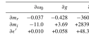
Table 1.Microphysics of spheres and spheroids considered in the MOPSMAP data set.
Method Mie TMM IGOM
Particle shape spheres oblate and prolate spheroids
0=1.2, 1.4, ..., 3.0, 3.4, 3.8, ..., 5.0 Size parameter 10−6< xc<1005 10−6< xc< (5−125) (5−125) < xc<1005
xi+1 xi =1.01
xi+1 xi =1.05
xi+1 xi =1.10
size bins single size single size
mr (0.1, 0.2, ..., 0.9, 1.0)∗, 1.04, 1.08, ..., 1.68, 1.76, ..., 2.0, 2.2, ..., 3.0
mi 0, 0.0005375, 0.001075, 0.0015203, 0.00215,
0.0030406, 0.0043, 0.0060811, 0.0086, 0.0121622, 0.0172, 0.0243245, 0.0344, 0.0486490, 0.0688, 0.0972979, 0.1376, 0.2752, 0.5504, 1.1008, 2.2016
∗IGOM was not applied tom≤1.0.
Table 2.Microphysics of irregularly shaped particles considered in the MOPSMAP data set.
Particle shape Shapes A–F, Fig. 1 of Gasteiger et al. (2011b)
Size parameter 10−3< xv<30.2;xi+xi1≈1.10; single size
mr 1.48, 1.52, 1.56, 1.60
mi 0, 0.00215, 0.0043, 0.0086, 0.0172, 0.0344, 0.0688
In summary, ADDA with the filtered coupled-dipole tech-nique, at least 11 dipoles per wavelength and a stopping cri-terion for the iterative solver of 10−3 was used for optical modeling of the irregularly shaped particles in our data set together with the orientation averaging scheme combining 206 ADDA runs. Tests demonstrate that the modeling accu-racy is mainly determined by the applied orientation averag-ing scheme.
2.3 Optical data set
Using the codes with the settings described above, a data set of modeled optical properties of single particles in ran-dom orientation was created. For spheres, we stored aver-ages over narrow size bins as described above instead of single particle properties. An overview over the wide range of sizes, shapes, and refractive indices of the particles in the data set is given in Tables 1 and 2. For each combina-tion of refractive index and shape a separate netCDF file was created, e.g., “spheroid_0.500_1.5200_0.008600.nc” for spheroids with m=0.5 (prolate with 0=2.0) and m= 1.52+0.0086i. Each file contains the optical properties on a grid of size parameters. The complete data set requires about 42 gigabytes of storage capacity.
For spheres and spheroids the minimum size parameter is set to 10−6, and the maximum size parameter is set to x≈1005 to cover, e.g.,rc=80 µm atλ=500 nm. The size
increment is 1 % (i.e.,xi+1/xi =1.01) in the case of spheres, 5 % in the case of TMM spheroids, and 10 % for IGOM spheroids. In the case of spheroids having refractive indices most relevant for atmospheric studies, the TMM is applied up to (or close to) the largest possible size parameter with the approach described in Sect. 2.2.2. The maximum size pa-rameter of the TMM calculations is reduced for less relevant refractive indices. An overview is given in Sect. S2 of the Supplement and a detailed list of the maximum size parame-ters for allmandmcombinations can be downloaded from Gasteiger and Wiegner (2018). The maximum size parame-ter for TMM is in the range 5< x <125, strongly depend-ing onmand particle shape, and determines the lowest size parameter at which IGOM may be applied. The first IGOM size parameter is between 0 and 10 % larger than the max-imum TMM size parameter. The TMM and IGOM results for spheroids are merged into a single netCDF file covering the complete size range fromx=10−6tox≈1005, which is sufficient for most applications. For example, for prolate spheroids with 0=1.8 and m=1.56+0i, the size range from x=10−6 to x=88.22 is covered by TMM; IGOM starts atx=89.54. The transition from TMM to IGOM for several scattering angles is demonstrated in Sect. S3 of the Supplement. Since IGOM is an approximation, unrealistic jumps of optical properties may occur at the transition. For typical mineral dust ensembles in the visible spectrum, par-ticles in the IGOM range contribute less than 10 % to the total extinction. IGOM was not applied tomr<1.04; thus, the size parameter range is limited to the TMM range for these refractive indices. A step of 0.04 was selected for the mr grid in the most relevant range (from 1.00 to 1.68) and a widermr step elsewhere. The development of the data set started withmi =0.0043, and beginning from this value,mi was increased and decreased in steps of a factor
√
The optical data for the irregularly shaped particles (Ta-ble 2) are limited toxv≤30.2 because of the huge
compu-tation requirements for optical modeling of large particles. Nonetheless, the most important range for many applications is covered; e.g., at λ=1064 nm particles up torv=5.1 µm
can be modeled. Themgrid for the irregularly shaped parti-cles is limited to the most relevant range for desert dust in the visible spectrum, and themi step is set to a factor of 2. The quantification of the conversion factor ξvc of the six
irreg-ular shapes requires the determination of their orientation-averaged geometric cross sections, which is done numeri-cally.
The optical properties stored for each particle are the ex-tinction efficiencyqext, the scattering efficiencyqsca, and the
expansion coefficientsαl1,αl2,α3l,α4l,β1l, andβ2l of the scat-tering matrix. The ADDA and the IGOM code provide the angular-resolved scattering matrix elements, which we con-verted to the expansion coefficients stored in the data set fol-lowing the method described by Hovenier and van der Mee (1983) and Mishchenko et al. (2016). We optimized the ex-pansion coefficients for accurate scattering matrices at 180◦, which is probably the most error sensitive angle. As a by-product, lidar applications will certainly benefit from this op-timization.
In the case of asymmetric shapes in random orientation, the scattering matrix has 10 independent elements as dis-cussed by van de Hulst (1981). By using only six elements of F(Eq. 8) in our data set, we implicitly assume that each irreg-ular model particle (shapes A–F) occurs as often as its mir-ror particle, which is formed by mirmir-roring at a plane (van de Hulst, 1981).
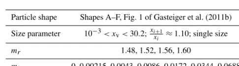
Figure 2 shows an example from the MOPSMAP optical data set. The refractive index is set tom=1.56+0.00215i, which is representative of desert dust particles at visible wavelengths. The properties of spherical particles are shown in blue, whereas the properties of prolate spheroids with0= 1.4 and 3.0 are shown in orange and green, respectively. Red and violet lines denote irregularly shaped particles D and F, respectively. Figure 2a shows the extinction efficiencyqextas
a function of cross-section-equivalent size parameterxc. The
general shape of theqext(xc)curve is similar for the different
shapes; nonetheless, with increasing deviation from a spher-ical shape, the amplitudes of the oscillations ofqext(xc)
be-come smaller and a shift in the maximumqexttowards larger
xcis found. Figure 2b shows the single-scattering albedoω0
for the same particles as Fig. 2a. For particle sizes compa-rable to the wavelength, ω0 reaches maxima with values of
about 0.991, almost independent of particle shape. ω0
ap-proaches a value of about 0.551 atxc≈1000 for spheres and
spheroids. Fig. 2c shows the asymmetry parameterg. When the particle size becomes comparable to the wavelength,g in-creases and oscillates as a function ofxc, with the strongest
oscillations occurring in the case of spheres. There is some shape dependence of g forxc>5; in particular, the
aggre-gate shape results in systematically smallergthan the other
100 101 102 103
0.0 0.5 1.0 1.5 2.0 2.5 3.0 3.5 4.0 4.5 5.0
Ex
ti
n
ct
io
n
e
ff
ic
ie
n
cy
q
ext SpheresProlate spheroids =1.40
Prolate spheroids =3.00
Aggregates (shape D) Edged particles (shape F)
100 101 102 103
0.5 0.6 0.7 0.8 0.9 1.0
S
in
g
le
-s
ca
tt
e
ri
n
g
a
lb
e
d
o
0
100 101 102 103
Size parameter
x
c0.0 0.1 0.2 0.3 0.4 0.5 0.6 0.7 0.8 0.9 1.0
As
y
m
m
e
tr
y
p
a
ra
m
e
te
r
g
(a)
(b)
(c)
Figure 2. Optical properties of single particles (or narrow size bins in the case of spheres) with fixed refractive indexm=1.56+
0.00215ias a function of size parameter. The different colors denote different particle shapes. Panel(a)shows the extinction efficiency
qext, panel(b)the single-scattering albedoω0, and panel (c)the
asymmetry parameterg.
shapes forxc>10. The transition from the numerically
ex-act TMM to the IGOM approximation occurs atxc≈125 for
0=1.4 (orange line) and atxc≈27 for0=3.0 (green line)
and is quite smooth.
3 MOPSMAP Fortran program
● Read input file ● Read data set index
Start
● Initialize λ grid and
refractive indices
● Initialize shapes ● Initialize sizes ● Consider hygroscopic
growth
For each wavelength:
● Decompose into contributions
from mr , mi , εm grid points
● Calculate optical properties
of aerosol ensemble
● Write
output
End
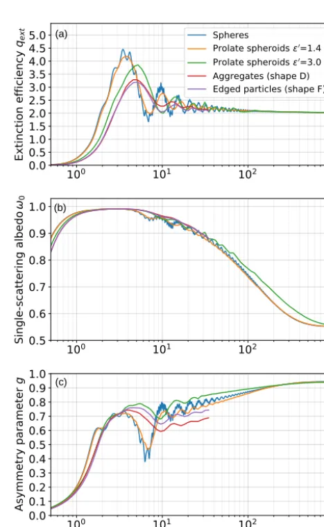
Figure 3.Simplified flow chart of the MOPSMAP Fortran program.
low for state-of-the-art personal computers. The Fortran code and the data set are available for download from Gasteiger and Wiegner (2018), and a web interface (see Sect. 4) pro-vides online access to most of the functionality of the Fortran program without the requirement of downloading the code and the data set.
Within each MOPSMAP run the optical properties of a specific defined ensemble are calculated at a user-defined wavelength grid. The ensemble microphysics and the wavelength grid are defined in an input file. The details about the options available for the input file are described in a user manual which is provided together with the code.
Figure 3 shows a flow chart of the MOPSMAP Fortran program. The program is initialized by reading the input file and a data set index. The latter contains information on the refractive index and shape grid and the size parameter ranges covered by the data set. Then, all information required for the optical modeling is initialized, for example the set of wave-lengths, the refractive indices as a function of wavelength, shape distributions, and the effect of the hygroscopic growth, before the optical calculations are performed for each wave-length, as described in the following.
3.1 Calculation of optical properties of particle ensembles
Usually aerosol particles occur as ensembles of particles of different size, refractive index, and/or shape. The different particles contribute to the optical properties of the ensem-ble. Assuming that the distance between the particles is large enough for interaction of light with each particle to occur without influence from any other particle (“independent scat-tering”; van de Hulst, 1981), the contribution of each particle can be added as described below.
In MOPSMAP particle ensembles are composed of one or more independent modes (the terms “mode” and “compo-nent” are often used synonymously in the literature). Each mode in MOPSMAP is characterized by particle size, shape, and refractive index, whereby each property can be described as a fixed value or as a distribution (see below). As these parameters do not necessarily correspond to the grid points of the MOPSMAP data set, for each mode (and each wave-length), decomposition into contributions from the different availablemand shapes of the data set needs to be performed. For a mode containing spheroids, in the most simple but probably most frequently used case of fixed values of mr, mi, andm, linear interpolation in the three-dimensional (mr, mi,m) space of the MOPSMAP data set is performed; i.e., eight grid points contribute to the result, with each grid point weighted according to the normalized distance from the pa-rameters of the mode. For each dimension, the contributing grid points are the nearest grid point smaller or larger than the value of the mode; e.g., for the real part of the refractive indexmr
mr,i≤mr< mr,i+1. (14)
The weight of the grid pointsmr,iandmr,i+1is
wmr,i=
mr,i+1−mr mr,i+1−mr,i
, (15)
wmr,i+1=
mr−mr,i mr,i+1−mr,i
. (16)
Finally the weights for each of the eight contributions are calculated as the products of the weights determined for each dimension. An example is shown in Sect. S4 of the Supple-ment. The error in the interpolation of the user-specified val-ues between the grid points of the data set is discussed in Sect. 3.3
because of the limited size range of irregularly shaped par-ticles in the data set, a special treatment can be applied: a MOPSMAP option is available which substitutes irregularly shaped particles above a selected size parameter with other particle shapes, spherical or nonspherical, as selected by the user. As a consequence, the particle shape of that mode be-comes size- and wavelength-dependent and the number of different contributions increases. The total number of con-tributions for an ensemble, denoted as J in the following, varies because the number of modes is not fixed and, as just discussed, the number of contributions from each mode de-pends on the characteristics of each mode. This underlines the flexibility of MOPSMAP.
The optical properties of the particle ensemble are calcu-lated for each wavelength by summation over extensive prop-erties of all particles described by theJ contributions. This approach corresponds to the so-called external mixing of par-ticles. Each contribution has a size distribution nj(r), i.e., a particle number concentration per particle radius interval fromrtor+dr, in the range fromrmin,j tormax,j, which is obtained by multiplying the user-defined size distribution of the mode with the weights obtained during the decomposi-tion. The extinction coefficientαextand the scattering
coeffi-cientαscaare calculated by
αext=
J
X
j=1
rmax,j
Z
rmin,j
Cext,j(r)·nj(r)·dr
, (17)
αsca=
J
X
j=1
rmax,j
Z
rmin,j
Csca,j(r)·nj(r)·dr
. (18)
The expansion coefficients need to be weighted with Csca,j(r); for example, α1l of a particle ensemble is calcu-lated by
α1l = 1 αsca
· J
X
j=1
rmax,j
Z
rmin,j
αl1,j(r)·Csca,j(r)·nj(r)·dr
. (19)
For the integration of extensive properties over the size dis-tribution, we apply the trapezoidal rule, which assumes lin-earity between thergrid points.
The size distribution n(r)=dN
dr for each mode can be specified in various ways. The MOPSMAP user can either specify a single size, apply size distribution tables in ASCII format, or apply a size distribution parameterization. The fol-lowing parameterizations are available:
1. n(r)=√1
2π N0
lnσ
1
rexp
−1
2
lnr−lnrmod
lnσ
2
– log-normal distribution;
2. n(r)=Arαexp(−Brγ) – modified gamma distribu-tion, Deirmendjian (1964);
3. n(r)=Aexp(−Br) – exponential distribution,α= 0,γ=1;
4. n(r)=Arα – power law distribution, Junge distribu-tion,B=0, Deirmendjian (1964);
5. n(r)=Arαexp(−Br) – gamma distribution,γ=1, Twomey (1977).
rmod is the mode radius, σ a dimensionless parameter for
the relative width of the distribution, andN0the total
num-ber density (in the range fromrmin=0 tormax= ∞) of the
lognormal distribution. For the subsequent size distributions, parametersA,α,B, andγ are positive andAcontrols the scaling of total number density whereasα,B, andγ are rel-evant for the shape of the size distributions. The exponential distribution, power law distribution, and the gamma distribu-tion are a subset of the modified gamma distribudistribu-tion with the specific parameter values as given above (see also Petty and Huang, 2011).
The particle shape can be specified independently for each mode and is, within each mode, independent of size and re-fractive index. In the case of spheroids, either a fixed aspect ratio0or an aspect ratio distribution is used. The latter can be given as a table in an ASCII file or it can be parameterized by a modified lognormal distribution (Kandler et al., 2007) n(0)= dN
N0·d0
= (20)
1 √
2π σar(0−1) exp
−
1 2
ln 0−1−ln 00−1 σar
!2
with parameters00 for the location of the maximum ofn(0) andσarfor the width of the distribution.
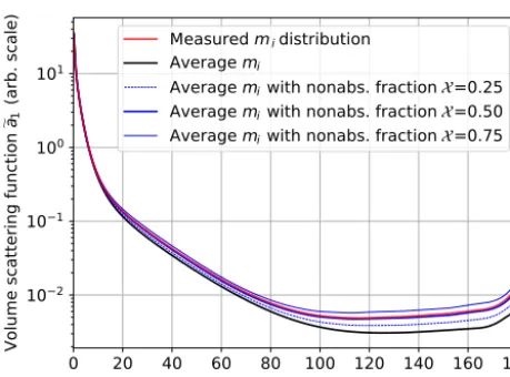
The refractive index of each mode can either be wavelength-independent or specified as a function of wave-length in an ASCII file. In addition, it is possible to spec-ify for each mode a non-absorbing fraction X. If X>0, the mode is divided, for all sizes and shapes, into a non-absorbing (mi,1=0, relative abundance X) and an
absorb-ing fraction (mi,2=mi/(1−X), relative abundance 1−X). As a consequence, the average mi over all particles of the mode remains equal to themi as specified by the user. This non-absorbing fraction approach can be used as a parameter-ization of the refractive index variability within desert dust ensembles as described by Gasteiger et al. (2011b) and be-low in Sect. 5.6.
For the hygroscopic particle growth the following param-eterization (Petters and Kreidenweis, 2007; Zieger et al., 2013)
rwet(RH)
rdry
=
1+κ· RH 1−RH
13
the size of the particle at a given RH and the size of the par-ticle in a dry environment (RH=0 %). The parameterization implies that this ratio is independent of size; thus, for exam-ple in the case of a lognormal size distribution, rmin,rmax,
andrmodare multiplied with this ratio, whereas the relative
widthσ of the distribution is not modified. This is the usual approach though modal representations of aerosol size dis-tributions may also predict higher moments (Binkowski and Shankar, 1995; Zhang et al., 2002), and thusσcan be a prog-nostic variable as well. The refractive index is modified by the water taken up following the volume weighting rule. Both RH andκ can be chosen by the user. This parameterization is valid for particles with r >40 nm, where the Kelvin ef-fect can be neglected (Zieger et al., 2013). It is worth noting that this parameterization differs from the relative humidity dependence implemented in OPAC, which was adapted from Hänel and Zankl (1979).
3.2 Output of Fortran program
As output of MOPSMAP the following properties of aerosol ensemble are available. Redundant properties, such as lidar-related properties, are available to facilitate the use of the results:
– extinction coefficientαext(m−1)
– single-scattering albedoω0
– asymmetry parameterg – effective radiusreff=
R r3n(r)dr R
r2n(r)dr (µm) (referring torc,rv, orrvcras selected by the user)
– number densityN(m−3) (number of particles per
atmo-spheric volume)
– cross section densitya(m−1) (particle cross section per atmospheric volume)
– volume densityv(particle volume per atmospheric vol-ume)
– mass concentrationM(gm−3) (particle mass per atmo-spheric volume)
– expansion coefficients (αl1toβ2l) for elements of scat-tering matrix
– scattering matrix elements (a1tob2) at user defined
an-gle grid
– volume scattering functionea1=αext4π·ω0·a1 (m−1sr−1)
at user defined angle grid – backscatter coefficientβ=αext·ω0
4π ·a1(180
◦)(m−1sr−1)
– lidar ratioS= 4π ω0a1(180◦)(sr)
– linear depolarization ratioδl=a1(180
◦)−a 2(180◦) a1(180◦)+a2(180◦)
– Ångström exponents AEζ = −
logζ (λ1) ζ (λ2)
logλ1 λ2
for ζ∈ {αext, αsca, αabs, β}
– extinction-to-mass conversion factorη= M αext (g m
−2)
– mass-to-backscatter conversion factor Z= β M (m2sr−1g−1).
Scattering matrix elements and the quantities derived from them are calculated from the expansion coefficients. Wavelength-independent propertiesreff,N,a,v, andMare
calculated for each wavelength to demonstrate the numerical accuracy of the integration.
The results are available in ASCII and in netCDF format. The format of the program output is described in the user manual. The netCDF output files can be read by the radia-tive transfer model uvspec, which is included in libRadtran (Mayer and Kylling, 2005; Emde et al., 2016).
3.3 Interpolation and sampling error
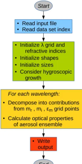
Due to the limited size resolution in the data set and re-quired interpolations between refractive index and aspect ra-tio grid points, deviara-tions from exact model calculara-tions for specific microphysical properties occur. As examples, Fig. 4 illustrates deviations introduced for single particle proper-ties, whereas Table 3 shows deviations for particle ensem-bles.
In Fig. 4a and c effects of the limited size resolution on the extinction efficiencyqextand the asymmetry parameterg
are shown for non-absorbing spheres and spheroids withm= 1.52+0i. In particular for spheres withx >10, deviations for single particles can be considerable because of small-scale features that are not resolved in the data set. In the case of spheres these features are implicitly considered in the data set by storing the average over 1000 sizes within each size bin as described above. In the case of spheroids, the data set contains properties calculated for single sizes which may not be fully representative of close-by sizes. However, since the small-scale features are much weaker for spheroids than for spheres, the average deviation for spheroids is much smaller than for spheres.
In Fig. 4b and d effects due to the required interpolation between the refractive index grid points are illustrated for spheres with m=1.54+0.005i. While the red lines show the properties calculated from the data set, the black lines show Mie calculations done explicitly form=1.54+0.005i with the same size grid as used in the data set. The compar-ison illustrates that MOPSMAP calculates optical properties on average correctly, but some smaller-scale features are lost: for example, the extinction efficiencyqext(x)in the size
0 5 10 15 20 25 30 35 40 0
1 2 3 4 5
x
ti
n
ct
io
n
e
ff
ic
ie
n
cy
E
qext (a)
m=1.52+0i Spheres at high size resolution
Prol. spheroids =2 at high size r.0
Spheres from data set
Prol. spheroids =2 from data set0
0 5 10 15 20 25 30 35 40
Size parameter xc
0.50 0.55 0.60 0.65 0.70 0.75 0.80 0.85 0.90
A
sy
m
m
e
tr
y
p
a
ra
m
e
te
r
g
(c)
0 5 10 15 20 25 30 35 40
0 1 2 3 4 5
E
x
ti
n
ct
io
n
e
ff
ic
ie
n
cy
qext (b)
Spheres
Data set grid points near m=1.54+0.005i Data set interpolated for m=1.54+0.005i Mie theory for m=1.54+0.005i
0 5 10 15 20 25 30 35 40
Size parameter xc
0.50 0.55 0.60 0.65 0.70 0.75 0.80 0.85 0.90
A
sy
m
m
e
tr
y
p
a
ra
m
e
te
r
g
(d)
Figure 4.Examples illustrating the effect of the limited size resolution of the MOPSMAP data set(a, c)and the effect of the interpolation between the refractive index grid points of the data set(b, d); extinction efficienciesqext(a, b)and asymmetry parametersg(c, d)as functions
of the size parameter fromx=0 tox=40 are compared; in(a)and(c)the high size-resolution calculations (black lines) were performed with linearxsteps of 0.002 in the case of spheres and 0.01 in the case of spheroids; in(b)and(d)the red lines show properties calculated with MOPSMAP form=1.54+0.005iby interpolation between refractive indices included in the data set (i.e., betweenm=1.52+0.0043i,
m=1.52+0.0060811i,m=1.56+0.0043i, andm=1.56+0.0060811i, for which the properties are shown as thin gray lines), and for comparison, the black lines show the properties calculated by Mie theory explicitly form=1.54+0.005iusing the samexgrid as used by the data set.
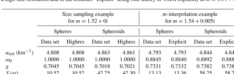
Table 3. Optical properties calculated for a lognormal mode withrmod=0.5 µm, σ=2.0,rmin=0.001 µm, and rmax=4 µm atλ=
628.32 nm. Two cases of particle shapes are considered: spheres and prolate spheroids with0=2.0. The columns “data set” contain values calculated using MOPSMAP with the data set described in Sect. 2.3. For comparison, the same properties are calculated in the columns “highres” using a high size resolution and in the columns “explicit” using Mie theory or TMM explicitly atm=1.54+0.005i.
Size sampling example m-interpolation example
form=1.52+0i form=1.54+0.005i
Spheres Spheroids Spheres Spheroids
Data set Highres Data set Highres Data set Explicit Data set Explicit
αext(km−1) 4.808 4.808 4.863 4.861 4.793 4.793 4.844 4.846
ω0 1.0000 1.0000 1.0000 1.0000 0.8845 0.8840 0.8892 0.8886
g 0.7045 0.7045 0.7018 0.7021 0.7331 0.7332 0.7382 0.7380
S(sr) 10.52 10.52 42.75 42.30 13.13 13.36 58.25 58.78
Mie calculation form=1.54+0.005ibecause of the inter-ference of the qext(x)curves for mr =1.52 andmr=1.56 (see gray lines in Fig. 4b; note that curves for differentmilie almost on top of each other).
For other size ranges, refractive indices, and optical quan-tities, the effects on the single particle properties are in prin-ciple similar but they may vary in magnitude.
Table 3 investigates the sampling and interpolation errors for a mono-modal lognormal size distribution with a typi-cal width ofσ=2.0. The effective radius isreff=1.44 µm,
which is a typical value for transported desert aerosol. Sizes up tormax=4 µm, which corresponds to size parameterxc=
40 atλ=628.32 nm, are considered. The left half of Table 3 compares optical properties calculated from the MOPSMAP data set (columns “data set”) with properties calculated using a high size resolution (columns “highres”), the same resolu-tions as displayed in Fig. 4a. For spheres, the results are equal up to at least the fourth digit. In the case of prolate spheroids with0=2.0, deviations are found for the fourth digit ofαext
and g. For the lidar-related quantities S and δl, the
differ-ences are larger with the relative deviation ofδlbeing 2.6 %.
These differences are caused by the high sensitivity of lidar-related quantities, and it is expected that deviations become smaller when shape distributions or wider size distributions are applied.
The right half of Table 3 demonstrates the effect of the m interpolation for an exemplary m=1.54+0.005i. MOPSMAP calculations (columns “data set”) are compared to results obtained using explicitly this refractive index in the Mie and TMM calculations. While the effect of them inter-polation is very small forαext,g, andδl, it is slightly larger
for ω0andS. The maximum relative effect is found for the
lidar ratioSof spheres with a deviation of 1.7 %.
These comparisons demonstrate that deviations found for single particles are largely smoothed out in the case of par-ticle ensembles due to the averaging over a large number of different particles. Only for a few special atmospheric appli-cations, for example, the modeling of a rainbow, the limited resolution of the data set may still lead to a considerable er-ror.
4 MOPSMAP web interface
A web interface is provided as part of MOPSMAP at https: //mopsmap.net. It was designed to be intuitive for expert and nonexpert users, e.g., for the demonstration of sensitivities of optical properties on microphysical properties in the frame-work of lectures, but also for a lot of scientific problems as outlined in the following section. The web interface is writ-ten in PHP and uses the SQLite library. After the registration as a user, online calculations of optical properties of a large range of particle ensembles can be performed. Input and out-put can be defined by the user; for nonexpert users, a lot of default ensembles representative of specific climatological
conditions are already available. The input parameters pri-marily include the microphysical properties of the particles. The particles’ microphysics are described by up to four com-ponents (each described by an individual lognormal size dis-tribution), the wavelength dependence of the refractive index and the shape. Any lognormal size distribution can be used; to facilitate the usage (e.g., for nonexpert users), the aerosol components from the OPAC data set (Hess et al., 1998), e.g., “mineral coarse mode”, “water-soluble”, or “soot”, are al-ready included. The same is true for the 10 “aerosol types” defined in OPAC, e.g., “continental clean”, “urban” or “mar-itime polluted”, consisting of a combination of components. Calculations can be made for a single wavelength, for wave-length ranges or a prescribed wavewave-length set (e.g., for a typi-cal aerosol lidar or a AERONET sun photometer). Moreover, users can define their own wavelength sets, e.g., for a specific radiometer. The relative humidity is selected by the user and it is effective for all hygroscopic components according to Eq. (21). The hygroscopic growth of the OPAC components in MOPSMAP differs from the original OPAC version (Hess et al., 1998); it follows theκparameterization with the values proposed by Zieger et al. (2013). In the “expert user mode” the flexibility is further increased: the number of components can be larger than four, and the size distribution can be given as discrete values on a user-defined size grid.
The output comprises the complete set of optical proper-ties as described in Sect. 3.2. It can be downloaded for further applications and includes ASCII tables as well as a netCDF file that can be used for radiative transfer calculations with uvspec of the widely used libRadtran package (Emde et al., 2016). To provide an immediate overview over the results, the most important parameters, such as extinction coefficient (αext), single-scattering albedo (ω0), asymmetry parameter
(g), Ångström exponent (AE), or lidar ratio (S), are displayed as tables when the calculations have been completed. In ad-dition plots of the results as a function of wavelength and scattering angle are shown as selected by the user.
All results are stored in the user’s personal folder so that all calculations can be reproduced. Furthermore, all calcula-tions can also easily be rerun with a slightly modified input parameter set.
5 Applications
In this section a selection of examples is presented to demon-strate the wide range of applications of MOPSMAP. Many of them can be performed by using the web interface. Some examples need a local version of MOPSMAP alongside with scripts that repeatedly call the Fortran program. These scripts are written in Python and can be downloaded from Gasteiger and Wiegner (2018) as part of the MOPSMAP package.
0 50 70 80 90 0 1 2 3 4 5 Normalized extinction
= 355 nm
desert arctic antarctic Urban Desert Arctic Antarctic
0 50 70 80 90
0 1 2 3 4
5 = 532 nm
contin. clean contin. average contin. polluted Contin. clean Contin. average Contin. polluted
0 50 70 80 90
0 1 2 3 4
5 = 1064 nm
maritime clean maritime polluted maritime tropical Maritime clean Maritime polluted Maritime tropical
0 50 70 80 90
0.6 0.7 0.8 0.9 1.0 S in g le -s ca tt e ri n g a lb e d o 0
0 50 70 80 90
0.6 0.7 0.8 0.9 1.0
0 50 70 80 90
0.6 0.7 0.8 0.9 1.0
0 50 70 80 90
0.0 0.5 1.0 1.5 2.0 2.5
Extinction to mass conversion
f a ct o r [ gm 2]
0 50 70 80 90
0.0 0.5 1.0 1.5 2.0 2.5
0 50 70 80 90
0.0 0.5 1.0 1.5 2.0 2.5
0 50 70 80 90
Relative humidity RH [%] 0.00 0.02 0.04 0.06 0.08 0.10 0.12
Mass to backscatter conver- s
io n fa ct o r Z [ m 2sr 1g 1]
0 50 70 80 90
Relative humidity RH [%] 0.00 0.02 0.04 0.06 0.08 0.10 0.12
0 50 70 80 90
Relative humidity RH [%] 0.00 0.02 0.04 0.06 0.08 0.10 0.12
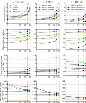
Figure 5.Properties of OPAC aerosol types as a function of relative humidity RH calculated with theκparameterization (Zieger et al., 2013) implemented in MOPSMAP (Eq. 21). The different colors denote the 10 different OPAC aerosol types as indicated in the legends. The columns denote different wavelengthsλas indicated above the upper row. The upper row shows the extinction coefficient normalized to the extinction coefficient of the same aerosol type at RH=0 % andλ=532 nm. The single-scattering albedoω0, the extinction-to-mass
conversion factorη, and the mass-to-backscatter conversion factorZare plotted in the subsequent rows.
Moreover, optical modeling is essential for many different re-lated modeling activities. It is required, for example, for clo-sure experiments (consistency checks between different mea-surement methods involving an aerosol model, e.g., Wiegner et al., 2009; Gasteiger et al., 2011b; Müller et al., 2012; Bell et al., 2013; Ma et al., 2014; Zieger et al., 2014; Düsing et al., 2018), radiative transfer studies (e.g., Otto et al., 2009; Emde et al., 2010), the inversion of remote-sensing measurements (e.g., Dubovik et al., 2006; Gasteiger et al., 2011a; Müller et al., 2016), the inversion of in situ data (e.g., Weinzierl et al., 2009; Szymanski et al., 2009; Kassianov et al., 2014), aerosol layer visibility simulations (e.g., Weinzierl et al., 2012), dynamic aerosol transport models (e.g., Heinold et al., 2007; Balzarini et al., 2015), aerosol characterization (e.g.,
Gasteiger et al., 2017; Che et al., 2018; Zhuang et al., 2018), and solar energy (e.g., Polo et al., 2016; Kosmopoulos et al., 2017).
5.1 Effect of hygroscopicity
ensem-bles and the relative humidity can be chosen by the user. MOPSMAP considers the hygroscopic effect by application of the κ parameterization (Eq. 21), which differs from the RH dependency implemented in OPAC.
The upper row of Fig. 5 shows the normalized extinction coefficient of the different types (indicated by color) at three wavelengthsλ(each in a subplot) calculated for RH values of 0, 50, 70, 80, and 90 %. The extinction at all λ is nor-malized to the extinction at RH=0 % andλ=532 nm. As a consequence, the differences between the columns illus-trate the wavelength dependency of the extinction, whereas changes with RH illustrate the hygroscopic effects. For ex-ample, for the desert aerosol type (orange color), the wave-length dependency is low, which is related to the large size of the dominant mineral particles, and the hygroscopic effect is relatively weak because mineral particles are hygrophobic. By contrast, for maritime (bluish colors) and antarctic types (purple color), the wavelength dependence is stronger and the hygroscopic effect is strong because of the domination by highly hygroscopic sulfate and sea salt particles. For the continental as well as the urban and arctic types, the wave-length dependence is even stronger and the hygroscopic ef-fect weaker, which may be explained by strong contributions from the soot and water-soluble components which contain quite small particles withκvalues significantly smaller than the κ values of sea salt particles (e.g., Petters and Kreiden-weis, 2007; Markelj et al., 2017; Enroth et al., 2018; Psi-choudaki et al., 2018).
The single-scattering albedo ω0 is shown in the second
row of Fig. 5. ω0 varies strongly with aerosol type, with
the highest values of almost 1.0 for the antarctic, maritime clean, and maritime tropical aerosol types. Since water is al-most non-absorbing at the considered wavelengths, the water uptake hardly changes ω0 ifω0is already close to 1.0. The
single-scattering albedo of the desert type is much lower, but it is also virtually independent on the RH as this aerosol type does not take up much water. For the other types, an increase in RH results in an increase inω0.
The extinction-to-mass conversion factorη, which is plot-ted in the third row of Fig. 5, is necessary to calculate mass concentrations from extinction coefficient measurements or mass loadings from AOD measurements. An important pa-rameter forηis the particle size (e.g., Gasteiger et al., 2011a) with the consequence that the desert aerosol type, which con-tains the highest fraction of coarse particles of the considered types, shows the highestηvalues. Again, the wavelength de-pendency is significant for the other aerosol types so that theηvalues atλ=1064 nm (right column) are significantly larger than atλ=532 nm (middle column). The dependence of ηon RH is significantly weaker than the dependence of the extinction on RH (upper row), which may be explained by the increase in mass with increasing RH compensating for the increase in extinction.
The bottom row of Fig. 5 illustrates the mass-to-backscatter conversion factorZas a function of RH.Zis
use-ful, for example, for comparisons of vertical profiles simu-lated with aerosol transport models to profiles measured with lidar or ceilometer. The multiplication of simulated aerosol mass concentrationMwithZ provides simulatedβ profiles which can be compared with the measurements. The figure shows that there is considerable spread between the different aerosol types, in particular at short wavelengths. RH only has strong effects on the maritime and arctic aerosol types.
Currently the hygroscopic growth of different aerosol components is not ultimately understood, and different κ-values are discussed. With MOPSMAP their influence on the optical properties can easily be determined and used in vali-dation studies.
5.2 Optical properties for sectional aerosol models
Aerosol transport models in combination with the optical properties of the aerosol allow one to model the radiative ef-fect of the aerosol. The aerosol is typically modeled in terms of mass concentrations for a limited number of aerosol types divided over a few size bins (sectional aerosol model) or a few modes (modal aerosol models). Thus, realistic optical properties for each size bin of each aerosol type are required for modeling the radiative effects (e.g., Curci et al., 2015).
In this example, we calculated the optical properties of dust at λ=500 nm for the five size bins of the COSMO-MUSCAT model (Heinold et al., 2007). The size bins are de-termined by the radius limits 0.1, 0.3, 0.9, 2.6, 8, and 24 µm. We assumed constant dv/dlnr within each bin. Each bin was modeled through the expert mode of the MOPSMAP web interface. The refractive index ism=1.53+0.0078i, which is equal to the value given for the mineral components in OPAC. We considered two cases for the particle shape: on the one hand, spherical particles and, on the other hand, pro-late spheroids with the aspect ratio distribution given by Kan-dler et al. (2009). For the latter case we assumed volume-equivalent sizes to keep the particle mass constant.
The calculated phase functions are presented in Fig. 6, where each size bin is represented by an individual color. The difference between both lines of the same color repre-sents the shape effect. For size bin 1 (0.1 µm< r <0.3 µm, black lines), the difference is small, whereas for all other bins the shape effect is larger. The strongest effects are found for θ >100◦with differences of up to a factor of 4 between the particle shapes. These angular ranges can be important, for example, for the backscattering of sunlight into space and thus for the aerosol radiative effect. The very strong effect at θ=180◦is relevant for any lidar application, e.g, the inter-comparison of modeled and measured attenuated backscatter profiles (Chan et al., 2018).
Calculated parameters relevant for radiative transfer and remote sensing are given in Table 4. The shape effect on the single-scattering albedoω0and the asymmetry parameterg
Table 4.Optical properties atλ=500 nm of the five COSMO-MUSCAT dust size bins. Two cases for the particle shape are considered: spheres/prolate spheroids. For details, see text.
Bin 1 Bin 2 Bin 3 Bin 4 Bin 5
ω0 0.9632/0.9628 0.9216/0.9264 0.7903/0.7934 0.6450/0.6485 0.5561/0.5601
g 0.6567/0.6585 0.6866/0.7111 0.8088/0.8109 0.8998/0.9017 0.9442/0.9419
η(g m−2) 0.2905/0.3000 0.5594/0.5236 2.230/2.071 6.989/6.633 22.09/20.90
Z(m2sr−1g−1) 4.234×10⁻²/ 1.185×10⁻¹/ 1.403×10⁻²/ 1.204×10⁻³/ 8.225×10⁻⁵/
3.981×10⁻² 5.421×10⁻² 8.901×10⁻³ 7.457×10⁻⁴ 8.651×10⁻⁵
0 20 40 60 80 100 120 140 160 180
Scattering angle
10 1
100
101
102
103
104
Ph
a
se
f
u
n
ct
io
n
a
1Bin 1, spheres Bin 1, spheroids Bin 2, spheres Bin 2, spheroids Bin 3, spheres Bin 3, spheroids Bin 4, spheres Bin 4, spheroids Bin 5, spheres Bin 5, spheroids
Figure 6. Phase functions at λ=500 nm of the five COSMO-MUSCAT dust size bins (different colors) assuming spherical par-ticles (solid lines) and prolate spheroids (dashed lines). For details, see text.
conversion factor η is systematically smaller for spheroids than for spheres in bins 2–5 because the geometric cross sec-tion of the spheroids is≈5.5 % larger than the cross section of the volume-equivalent spheres. The mass-to-backscatter conversion factorZ of the spheroids is lower than theZof spheres for most size bins, with maximum differences being larger than a factor of 2.
5.3 Effect of cutoff at maximum size
Many in situ measurement setups are limited with respect to the maximum particle size they are able to sample, e.g., because of losses at the inlet or the tubing. In this example, we illustrate the effect of the cutoff for the desert aerosol type from OPAC at RH=0 % (Koepke et al., 2015).
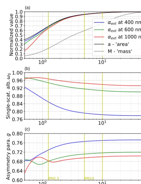
Figure 7 illustrates various aerosol properties as a func-tion of the cutoff radius rmax. Fig. 7a shows properties that
are normalized by the values found atrmax=60 µm (where
99.988 % of the total particle cross section is covered, refer-ring tormax= ∞). The PM10mass, i.e., the mass in the
par-ticles with diameter smaller than 10 µm (rmax=5 µm), and
the PM2.5mass (rmax=1.25 µm) are standard parameters to
quantify pollution (e.g., Querol et al., 2004). In our example,
100 101
0.0 0.1 0.2 0.3 0.4 0.5 0.6 0.7 0.8 0.9 1.0
Normalized value
ext at 400 nm
ext at 600 nm
ext at 1000 nm a - 'area' M - 'mass'
100 101
0.76 0.80 0.84 0.88 0.92 0.96 1.00
S
in
g
le
-s
ca
t.
a
lb
.
0
100 101
Cutoff radius
r
max [ m] 0.600.64 0.68 0.72 0.76 0.80
As
y
m
m
e
tr
y
p
a
ra
.
g
PM2.5 PM10
(a)
(b)
(c)
Figure 7.Optical and microphysical properties of the OPAC desert aerosol type as a function of cutoff radiusrmax. Panel(a)shows
the normalized extinction coefficientαextat three wavelengths, the
normalized cross section densitya, and the normalized mass con-centrationM. Normalization to values calculated forrmax=60 µm.
The single-scattering albedoω0at the same wavelengths is plotted
in(b), and the asymmetry parametergin(c).
PM10 and PM2.5 contain only 59.5 and 21.6 % of the total
particle mass, respectively. However, PM10and PM2.5
mea-surement setups cover 94.4 and 69.0 % of the total geomet-ric cross section, respectively. The single-scattering albedo in the case of PM2.5is about 0.035–0.071 higher than for the
Table 5.Properties of one-modal size distribution atλ=532 nm consisting of spheres or aggregate particles (shape D,ξvc=0.8708; Fig. 1
of Gasteiger et al., 2011b) assuming different size equivalences. For details, see text.
Properties Spheres Aggregate particles
Usingr Usingrc Usingrv Usingrvcr
αext(km−1) 0.350 0.347 0.449 0.750
ω0 0.897 0.922 0.910 0.883
g 0.722 0.679 0.680 0.689
a1(0◦) 100 97.4 128 222
ea1(0
◦) (km−1sr−1) 2.51 2.48 4.17 11.7
a1(180◦) 1.21 0.405 0.420 0.432
S(sr) 11.6 33.6 32.8 33.0
δl 0.000 0.450 0.454 0.454
Cross section densitya(km−1) 0.141 0.141 0.186 0.323
Mass concentrationM(µg m−3) 482 318 481 1103
of the mass are covered; the single-scattering albedo and the asymmetry parameter deviate from the total aerosol by less than 0.008.
This example shows that consideration of maximum size is essential when derived optical properties or mass concentra-tions are interpreted, and results can be severely misleading if the cutoff radius is not considered. These effects can be easily quantified with MOPSMAP and its web interface.
5.4 Effect of the selection of size equivalence of nonspherical particles
This example demonstrates how the selection of the size equivalence in the case of nonspherical particles affects var-ious ensemble properties. In MOPSMAP the size-related pa-rameters are either interpreted asrc(default) or asrvorrvcr
(see Sect. 2.1) according to the choice of the user. Each size equivalence can be transformed into another by Eqs. (3) and (4). For example, if “volume cross section ratio equivalent” has been chosen in the web interface, and “0.5” forrmod, this
would be equivalent to setting 0.5·ξvc−3 for rmod when the
default “cross section equivalent” is kept (ξvcdepending on
shape).
To further elucidate the role of the different representa-tions of radii, the same parameters of a lognormal size dis-tribution are applied to the different size interpretations. For this purpose, the parameters are set tormod=0.5 µm andσ=
2 with rmin=0.001 µm, rmax=1.75 µm (reff=0.98 µm),
andN0=103.66 cm−3, which results in a concentration of
N =100 cm−3in the range fromr
mintormax. The effect of
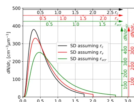
the three alternative interpretations on particle size is demon-strated in Fig. 8 for irregular shape D having ξvc=0.8708.
All three size distributions (curves of different color) are plotted in terms of dN/drc(rc)(black axes). For comparison,
axes for dN/drv(rv) (red axes) and dN/drvcr(rvcr) (green
axes) are also shown. Using these axes, the size distribution curves can be interpreted in terms of the various size
equiva-0.0 0.5 1.0 1.5 2.0 2.5 3.0
r
c [ m]0 100 200 300 400 500
dN
/
dr
c[
cm
3
m
1]
r
c0.5 1.0 1.5 2.0 2.5
r
v0.5 1.0 1.5 2.0
r
vcr0.5 1.0 1.5
dN
/
dr
c100
200
300
dN
/
dr
v100
200
300
dN
/
dr
vcr
100
200
300
400
SD assuming
r
cSD assuming
r
vSD assuming
r
vcrFigure 8.Lognormal size distributions (SD) with samermod, σ,
N0, and rmaxassuming different size equivalences for aggregate
particles (shape D,ξvc=0.8708) as applied in Table 5. The size
distributions are plotted in terms of cross-section-equivalent sizes (i.e., dN/drc(rc)referring to black axes and grid). For comparison
axes valid for the other size interpretations are also plotted in red and green, which allows each size distribution to be interpreted in terms of each size equivalence.
lences. The comparison between the size distributions clearly shows a shift towards larger sizes whenrvcrorrvinstead of
rcis assumed. For example, assumingrvcrfor the lognormal
size distribution (green curve) describes the same ensemble as usingrmod=ξvc−3·0.5 µm=0.8708
−3·0.5 µm=0.757 µm
(see Eq. 4) andrmax=0.8708−3·1.75 µm=2.65 µm when
assumingrcas particle size.