An ANOVA Based Analytical Dynamic Matrix Controller Tuning Procedure for FOPDT Models

An ANOVA Based Analytical Dynamic Matrix Controller

Tuning Procedure for FOPDT Models

Peyman Bagherii* and Ali Khaki-Sedighii

Received 5 October 2010; received in revised 21 November 2010; accepted 26 December 2010

i*

Corresponding author, P. Bagheri is with Advanced Process Automation & Control (APAC) Research Group of K. N. Toosi University of Technology, Tehran, Iran (phone: +98-21-84062161; e-mail: [email protected], [email protected]).

ii

A. Khaki-Sedigh is with Advanced Process Automation & Control (APAC) Research Group of K. N. Toosi University of Technology, Tehran, Iran, (e-mail: [email protected]).

ABSTRACT

Dynamic Matrix Control (DMC) is a widely used model predictive controller (MPC) in industrial plants. The successful implementation of DMC in practical applications requires a proper tuning of the controller. The available tuning procedures are mainly based on experience and empirical results. This paper develops an analytical tool for DMC tuning. It is based on the application of Analysis of Variance (ANOVA) and nonlinear regression analysis for First Order plus Dead Time (FOPDT) process models. It leads to a simple formula which involves the model parameters. The proposed method is validated via simulations as well as experimental results. A nonlinear pH neutralization model is used for the simulation studied. It is further implemented on a laboratory scale control level plant. A robustness analysis is performed based on the simulation results. Finally, comparison results are provided to show the effectiveness of the proposed methodology.

KEYWORDS

Dynamic Matrix Control, Tuning, Analysis of Variance (ANOVA), Nonlinear Regression, FOPDT, industrial processes, pH process, Level process.

1. INTRODUCTION

Model Predictive Control (MPC) strategies are widely used in industry as Advanced Process Controllers (APC) [1]. Dynamic Matrix Control (DMC) is the most popular MPC method in many chemical processes. This popularity is due to the simple structure of the controller. DMC uses step response information and in stable industrial processes, this is easily obtained. DMC, as a model predictive controller, was first proposed in [2]. As other MPC methods, DMC uses a prediction model. This model is a step response model. The next element in MPC is the objective function [3]. It is desired that the future output values on the considered horizon follow a desired reference trajectory and in the same time, the control effort is penalized properly.

MPC tuning is dealt with in several papers. In [4], some practical approaches to tuning MPC methods are presented. Reference [5] presents an on-line DMC tuning method. In [6], a method called the response surface

(GPC) for Second Order plus Dead time (SOPDT) models and a new analytical equation for λ is obtained. A review paper on different tuning methods for MPC can be found in [12].

This paper proposes a three stage procedure for determining a closed form formula for DMC tuning. In the first stage a bank of FOPDT models are simulated to test the effect of different model parameters on the tuning parameterλ. In the second stage, ANOVA is performed on these data to determine the most effective plant parameters on the tuning parameter. Finally, in the third stage, with some insights, nonlinear regression is employed to obtain a simple but precise tuning equation for λ.

In the following section, the DMC fundamentals are briefly reviewed. In section 3, the previous tuning methodologies are studied. An introduction to ANOVA is given in section 4, and the analytical ANOVA based tuning formula is then derived. Finally, simulation and experimental results are given in section 5.

2. DYNAMIC MATRIX CONTROL

DMC was developed at Shell Oil in the early 1970s. In 1979 Cutler and Ramaker [2] presented an unconstrained multivariable predictive controller which they named Dynamic Matrix Control (DMC). In this section, single input-single output (SISO) formulation of the DMC is briefly reviewed, for more details see [3].

Let the step response of a system be described as follows

(1)

( )

∞

(

)

= ∆ −

=

0

i gi ut i

t y

where gi are the sampled output values for the step

input, u

( )

t is the control signal and

( )

=

( )

−

(

−1

)

∆ut ut ut . The output prediction values along the finite horizon will be as

(2)

(

t k t

)

g u

(

t k

)

f

(

t k

)

y k

i i∆ + − + +

= +

=1 1

| ˆ

where f

(

t+k

)

is the free response of the system, and is given by (3)

(3)

(

t k

)

(

g g

) (

ut i

)

y

( )

t

f m

N

i k i− i ∆ − +

= +

=1 +

where ym is the real output value. We havegk+i−gi≈0

N i>

, where, N is the model horizon. In vector form we have

(4)

(

)

(

)

(

)

( )

(

)

(

)

(

)

(

)

(

)

=

+ + +

=

+ ∆

+ ∆

∆

=

+ + +

= + =

+ − −

−

1 1

1 1

1 2 1

0 0 0

, 1 1

1 ,

| ˆ

| 2 ˆ

| 1 ˆ ˆ ˆ

M P P

P M M

g g

g

g g

g g g g

P t f

t f

t f

M t u

t u

t u

t P t y

t t y

t t y

G f

u y

f Gu y

where P is the output horizon, M is the control horizon and G is the dynamic matrix. The quadratic objective index is

(5)

(

)

(

)

[

]

(

)

[

]

= =

− + ∆ +

+ − + =

M j P j

j t u

j t w t j t y J

1 1

1 |

λ

where w is the desired reference trajectory and λ is the move suppression coefficient that is an important tuning parameter in DMC. Control signal is calculated as

(6)

(

)

(

)

(

)

(

)

(

+

)

+ +

=

− +

= −

P t w

t w

t w

T T

2 1

1

w

f w G I G G

u λ

Hence, the DMC tuning parameters can be listed as

N M P, , ,

λ and T_s. Note that T_sis the sampling time.

3. DMCTUNING METHODS

There are several proposed tuning strategies in the literature, but only two of these methods have a sound mathematical background and provide an analytical expression for the tuning parameters of DMC. In this section, these two tuning methods are studied and tested via simulation examples.

Consider the approximated FOPDT model of the system as

(7)

( )

1 + =

−

s Ke s G

s m

τ θ

TABLE 1

DMCTUNING EQUATIONS (PREVIOUS WORKS) Parameters (Shridhar and Cooper) [8] (Iglesias et al) [10]

s

T

2 10

θ τ

≤

≤ s

s andT

T

2 10

θ τ

≤

≤ s

s andT

T

N P=

1 5

+ =

+ = =

s s

T k

k T N P

θ τ

1 5

+ =

+ = =

s s

T k

k T N P

θ τ

M Integer, from 1 to 6 Integer, from 1 to 6

λ 2

fK

4094 . 0 631 . 1

τ θ

K

f

0 1

3.5 5

1

500 s 2

M

M M

M T

τ

=

−

− > -

As it is shown in Table 1, the only difference in these formulae is in the equation forλ.

The formula for N is first studied. Consider process1 described in [8] by the following transfer function

(8)

( )

(

150 1

)(

25 1

)

50

+ + =

−

s s

e s

G

s

m

Figure 1 shows the effect of smallN. It is shown that the damping transient response repeats every N sample, also it is easily seen that if N gets smaller, this repetitive responses would be undesirable. So if it is possible, it is desirable to chooseN>5τ Ts+k. The proposed value

for N by Shridhar and Cooper in reference [8] is not large enough, which is one of the deficiencies of the proposed approach.

750 1000 1250 1500 1750 2000 2250 2500

0 0.2 0.4 0.6 0.8 1 1.2 1.4

Time (sec)

Y

Reference

(Shridhar and Cooper, 1997)

1000 1250 1500 1750 2000 2250 2500

0 0.2 0.4 0.6 0.8 1 1.2 1.4

Time (sec)

Y

Reference

(Shridhar and Cooper, 1997)

Figure 1: Effect of smallN.

Next, consider the equation for λ in Table 1 which is proposed by Shridhar and Cooper in reference [8]. In this equation, performance is not considered and a fast response with large overshoot in control signal is encountered. To be precise, in this equation if the

s

T

τ term gets smaller by increasing the amount delay, a larger sampling time and a very small λ are achieved and it yields a fast response that is not desirable for a system with large delays.

The proposed tuning method for λ by Iglesias et al. in reference [10] is shown in Table 1. It is noted that:

• It is shown in [8] that_λ=fK2_{. Formulation in}

[10] shows that, this relation is linear, i.e.,

K f1

=

λ . With a simple example we can show that if K get small enough, the closed loop responses becomes very slow.

• If K becomes large, the formulation in [10] leads to a smallλ and leads to a fast output response of the system.

• In the case of small enough delays in comparison with plant time constant, λ will be very small which yields a very fast response.

• In [10] using the analysis of variance (ANOVA), it is shown that the parameter Γ (defined later) is not efficient. This is because K is used in ANOVA and also the range of Γ is not sufficient. We will show that this parameter is very important and has an effective influence on the closed loop response.

To study the equation for λ in [10], see Table 1, we consider three different examples. The following FOPDT model is used in example 1

(9)

( )

1 10

005 . 0

+ =

−

s e s

G

s

Note that in this example, we haveK =0.005. According to [8], for this system we have _7.08 −7

= e

λ . And

according to [10], we have _3.2 −3

= e

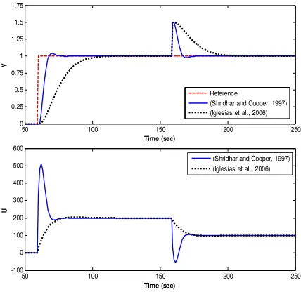
λ . Note that all the tuning parameters are calculated according to Table1. Figure 2 shows the results of these two tuning methods. In this example, both the set point tracking and disturbance rejection properties are the control objectives. It is shown that formulation in [10] leads to a very slow response. Also, it is seen that the method in [8] yields a fast response with high control signal overshoot, which is not acceptable in the practice.

N=40

N=28

N Sample

50 100 150 200 250 0

0.25 0.5 0.75 1 1.25 1.5 1.75

Time (sec)

Y

Reference

(Shridhar and Cooper, 1997) (Iglesias et al., 2006)

50 100 150 200 250

-100 0 100 200 300 400 500 600

Time (sec)

U

(Shridhar and Cooper, 1997) (Iglesias et al., 2006)

Figure 2: Closed loop responses (example 1).

In the second example, the following FOPDT is considered

(10)

( )

1 50

+ =

−

s e s G

s

In this example, system has a large gain value, K=50 According to [8], for this system we haveλ=578.9. And according to formulation in [10], we haveλ=81.5. As it mentioned, formulation in [8] always leads to a fast response but in this case formulation in [10] leads to a very fast response, see Fig. 3. These two examples show the high sensitivity of the method in [10] to the gain of system.

In example 3, we consider a system with no delay

(11)

( )

1 10

1 + =

s s

G

According to Table 1, formulation in [10] leads to λ=0

and method in [8] leads toλ=0.29. Fig. 4 shows the results of these methods, it is seen that formulation in [10] is not acceptable for the systems with no delay. Because it yields a very fast response and also a large overshoot in the control signal, which is not acceptable and executable in practice.

6 9 12 15 18

0 0.5 1 1.5 2

Time (sec)

Y

Reference

(Shridhar and Cooper, 1997) (Iglesias et al., 2006)

6 9 12 15 18

-0.02 0 0.02 0.04 0.06 0.08

Time (sec)

U

(Shridhar and Cooper, 1997) (Iglesias et al., 2006)

Figure 3: Closed loop responses (example 2).

50 55 60 65 70 75 80 85 90 95 100

0 0.2 0.4 0.6 0.8 1 1.2 1.4 1.6

Time (sec)

Y

Reference

(Shridhar and Cooper, 1997) (Iglasias et al., 2006)

50 55 60 65 70 75 80 85 90 95 100 -5

0 5 10 15

Time (sec)

U

(Shridhar and Cooper, 1997) (Iglasias et al., 2006)

Figure 4: Closed loop responses (example 3).

These simulations show that the methods in [10] and [7][8] can both give improper tuning parameters. In this paper, a new method is now presented to overcome the above mentioned problems. The main idea in this paper is using ANOVA and some insights to find an appropriate nonlinear fitting that is sufficiently accurate and simple. To find an analytical expression forλ, FOPDT model of the plant is used. Note that all the parameters of Table 1 except λ andN, are properly adopted. For λ a new equation will be determined, but N should only be larger than what it is in Table1, empirically N=2

(

5τ Ts

)

+k is

a good choice.

4. THE PROPOSED TUNING PROCEDURE

In this section, an introduction to the Analysis of Variance (ANOVA) is given. Then, the new tuning procedure is presented in details.

A. Analysis of Variance (ANOVA)

dependent variable. ANOVA capabilities were first introduced in [15]-[16]. In [16][17], ANOVA is used for path-finding, and it is used in soft computing in reference [18], also in [19] microwave applications of ANOVA can be found. In [20] ANOVA is used to tune the Generalized Predictive Controllers (GPC) for FOPDT plants. More recently, [11] has employed ANOVA for tuning of Generalized Predictive Controller (GPC) for Second Order plus Dead time (SOPDT) models and a new analytical equation for is obtained.

Here we deal with fixed-effect model of ANOVA [21]. The fixed-effects model of analysis of variance applies to situations in which the experimenter applies one or more treatments to the subjects of the experiment to see if the response values change.

Some basic definitions of reference [13] and [14] about ANOVA are given bellow.

Between groups variance is conceived in terms of the average of the differences amongst the means of the experimental conditions. Consequently, in each experimental condition there would be n_i experimental condition mean scores.

(12)

(

)

= −

= k

i i i

B n x x

SS

1

2

Between groups degree of freedom is defined as follows (13) 1

− =k dfB

where k is the number of groups.

Mean square between groups is defined as follows (14)

B B B

df SS S 2=

Within groups variance is defined as follows

(15)

(

)

= −

= k

i i i

W n S

SS

1

2

1

where S_i2 is the variance of each group.

Within groups degree of freedom is defined as follows (16)

k N dfW= −

where N is the total number of observations.

Mean square within groups is defined as follows (17)

W W W

df SS S 2=

And finally, the F-test is defined as

(18)

2 2

W B

S S F=

F_test is used for comparisons of the components of the total deviation. For example, in one-way or single-factor ANOVA, statistical significance is tested for by comparing the F-test statistic.

One-way ANOVA is used to test for differences among two or more independent groups.

In the simple case of the one-way ANOVA, the model is

represented as

(19)

ij i

ij G

y =µ+ +ε

where y_ij is the thj response in treatment group i, Gi

the deviation of the thi treatment (group) mean from the overall mean, µ; ε_ij the random error in the experiment (measurement error, biological variability, etc.) assumed to be normal with mean 0 and variance σ2.

In N-way ANOVA it is determined whether data mean in a set of data changes when factors and their different combinations are grouped together. If so, it can be verified which factors or combinations of factors are associated with the mean changes [13]. In other words, the effects of multiple factors on the mean of data are measured.

For example in the three-way ANOVA, the model is represented as

(20)

( )

( )

ik

( )

jk

(

)

ijk ijkl

ij k j i ijkl

y

ε αβγ βγ

αγ

αβ γ β α µ

+ +

+ +

+ + + + =

In this paper, two-way ANOVA is used as the main tool for statistical analysis of the data.

B. The Proposed Tuning Strategy

According to [8], we haveλ=fK2. Note that f is a scalar. So, in the following we consider only system delay and time constant of FOPDT and the goal is to find an optimal equation forf .

Now we construct the model bank, as all the possible combinations of the parameters shown in Table 2, overall we have 7×52=175 models. For each model appropriate parameters according to Table 1 are chosen, except forf . For each model, f varies from 0.05 to 10 and performance index (21) is calculated. Finally, the optimal value of is obtained for every model. The optimal value of minimizes the performance index (21).

(21)

( )

( )

(

)

∞

(

( )

)

∞

∆ Γ + −

=

0 2 0

2

dt t u dt

t y t r

J

TABLE 2

SETUP OF PARAMETERS FOR ANOVA

ANOVA Parameters

Level Low

Level Low Medium

Level Medium

Level Medium

High Level High

τ 10 40 80 120 160

θ 2 5 15 40 80

Γ 0.1 0.2 0.5 1 2 3 5

Results of ANOVA show that which one of model parameters or a combination of model parameters has more influence on the optimal tuned parameters and also the level of influence are determined by ANOVA. The result of ANOVA analysis is depicted in Table 3. In this table, there are F-values and P-values associated with each parameter and combination of parameters. These values reveal the effect and also the effectiveness level of these parameters on the optimally tuned parameters.

TABLE 3

ANOVARESULTS FOR DMCTUNING

Source Sum Sq. d.f. Mean Sq. F Prob>F

τ 0.743 4 0.186 26.18 5.84e-16

θ 0.577 4 0.144 20.34 4.71e-13

Γ 316.43 6 52.74 7431.6 0

θ

τ × 0.418 16 0.026 3.68 1.53e-5 Γ

×

τ 1.706 24 0.071 10.01 1.29e-19 Γ

×

θ 1.327 24 0.055 7.79 1.19e-15 Error 0.93 131 0.0071

Total 322.13 209

Typically there is a cut-off value of 0.05 for P index. That is, any of these sources having a value below the cut-off is considered to be significant. Also, a source with small P value and larger F value has larger influence on optimally tuned parameter. The remaining terms are omitted. According to Table 3 it is shown that, Γ is the most efficient parameter. Effect of θ and τ are countable. To have a simple formulation, combinations of parameters are not considered.

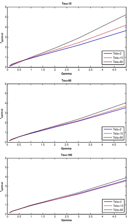
Now, we try to find a nonlinear meaningful function of these parameters. For this propose, Fig. 5 is checked in details. In this figure the optimal value of is shown in terms of the plant model parameters. Hence, primary formulation for f is in the form of (22)

(22)

b

a f = Γ

In this formulation a and b are not constant, they are a function of the other parameters of the system model.

• For a fixed time constant, increasing system delay leads to larger f .

• Plots comparisons show that increasing time constant, decreases the above effect, which means that θ τ is an important parameter in f and not

θ and τ individually.

• With the above observations, we consider

(

)

(

₄

)

5

(

(

)

₈

)

9

7 6 3

2

1 ,

x x x

x

x x b x

x x

a= + θ τ = + θ τ in a very general form. In this equation, xi is

obtained using nonlinear regression techniques.

0 0.5 1 1.5 2 2.5 3 3.5 4 4.5 5 0

1 2 3 4 5 6

Tau=10

Gamma fop

ti

m

a

l

Teta=2 Teta=15 Teta=80

0 0.5 1 1.5 2 2.5 3 3.5 4 4.5 5 0

1 2 3 4 5 6

Gamma fop

ti

m

a

l

Tau=80

Teta=2 Teta=15 Teta=80

0 0.5 1 1.5 2 2.5 3 3.5 4 4.5 5

0 1 2 3 4 5 6

Gamma

fop

ti

m

a

l

Tau=160

Teta=2 Teta=15 Teta=80

Figure 5: Optimal f via other parameters.

These observations and some tests lead to a simple formulation for f given below

(23)

0.15

2 0.9

, 0.84 0.94

f K f θ

λ

τ

= = + Γ

This formulation is obtained using a nonlinear regression. To show the accuracy of this formulation we compared the optimal values of f with the values obtained from (23), see Fig. 6. In Fig. 6, it is shown that the proposed formulation is accreted enough.

60 70 80 90 100 110 120

0 1 2 3 4 5

Number of Models

fop

ti

m

a

l

Optimal value Estimated

This formulation removes the deficiencies of the equation of [10], for example for a very small delay in comparison with time constant, this formulation yields to

(24)

9 . 0 2_{, =0.825Γ}

= fK f

λ

However, formulation in [10] yieldsλ=0. Also, using the parameterΓ, desired responses can be achieved; this capability dose not exists in [8] and [10]. To have a simpler formulation, three different values are chosen forΓ. We name Γ=0.1 as the output error importance,

1

=

Γ as intermediate and Γ=10 as the control effort importance. With these notations, we have

(25)

0.15 2

0.94

0.11 Output error importance : 0.1

0.84 Intermediate: 1

6.67 Control effort importance: 10

aK a θ λ τ = + Γ = = Γ = Γ =

In the special case, where the system delay is smaller than its time constant, (25) would be simpler

(26) = importance effort Control 608 . 6 te Intermedia 832 . 0 importance error Output 105 . 0 2 2 2 K K K λ

5. SIMULATION AND EXPERIMENTAL RESULTS

A. Simulation Results

In this section, the proposed tuning method is tested via simulation study of a pH neutralization process [22]-[23]. A schematic diagram of the pH neutralization process is depicted in Fig. 7.

This process is a well-known and standard bench mark system for comparing single loop and also multivariable control strategies. Here, we deal with the single input-single output pH process. The process consists of acid, base and buffer streams that are mixed in a vessel. In the SISO case, acid (HNO3) steam is a measured system

disturbance, base (NaOH) steam is the control signal and a buffer (NaHCO3, NaOH) stream is unmeasured

disturbance of system.

2

u

3

u

1

u

pH

h

Figure 7: pH neutralization schematic.

The control objective is to control the value of the pH of the outlet stream. It is assumed that the level of the solution in Continues Stirred Tank Reactor (CSTR) is fixed. The acid, base and buffer flow rates are presented respectively by u3,u1 andu2. It is proposed that the pH

of the outlet stream is measured at a distance from the plant, which introduces a measurement time delayθ. The dynamic model for reaction invariants of the effluent solution (w_a,w_b) is given by (27)

(27)

( )

( )

( )

[

]

[

]

( )

(

)

(

)

( )

(

) (

)

( )

(

) (

)

T b a T b a T b a T b a T x w V x w V x p x w V x w V x g x w V u x w V u x f w w x x x u x p u x g x f x − − = − − = − − = = = + + = 2 2 1 2 2 1 1 1 2 3 3 1 3 3 2 1 2 1 1 , 1 1 , 1 , , ,

The static part of this process is given by

(28)

(

)

(

)

2 1 2 10 10 1 10 2 1 10 10

, 14 2

1 pk y y pk

pk y y y x x y x

h _{− −}

− − − + + × + + − + =

In (28), pk1 and pk2 are the first and second

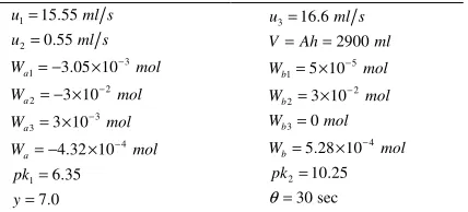
disassociation constants of the acid, respectively. The nominal pH parameters and operating conditions are given in Table 4.

TABLE 4

NOMINAL PHPROCESS OPERATING CONDITIONS

0 . 7 35 . 6 10 32 . 4 10 3 10 3 10 05 . 3 55 . 0 55 . 15 1 4 3 3 2 2 3 1 2 1 = = × − = × = × − = × − = = = − − − − y pk mol W mol W mol W mol W s ml u s ml u a a a a sec 30 25 . 10 10 28 . 5 0 10 3 10 5 2900 6 . 16 2 4 3 2 2 5 1 3 = = × = = × = × = = = = − − − θ pk mol W mol W mol W mol W ml Ah V s ml u b b b b

This process is highly nonlinear and the control objective is to achieve pH=7. Through an open loop step test, we can find the linear model of pH process around this operating point as

(29)

( )

1 85 497 . 0 30 + = − s e s G s

and control signals are shown in this figure.

Table 5 also summarizes the properties of different tuning methods. In this table, IAE is integral absolute error of output, _u2

shows the control signal energy,

∆_u2 _{shows the control effort energy, OV stands for the}

overshoot and finally TS means settling time with criteria of 2%. These parameters are considered for tracking from pH=7.2 to pH=7.

0.8 0.9 1 1.1 1.2 1.3 1.4 x 104 6.6

6.7 6.8 6.9 7 7.1 7.2 7.3 7.4

Time (sec)

p

H

Reference

(Shridhar and Cooper, 1997) (Iglesias et al., 2006) Proposed (Gamma=1) Proposed (Gamma=10) Proposed (Gamma=0.1)

0.8 0.9 1 1.1 1.2 1.3 1.4 x 104 14

14.5 15 15.5 16 16.5 17 17.5 18

Time (sec)

B

a

s

e

(Shridhar and Cooper, 1997) (Iglesias et al., 2006) Proposed (Gamma=1) Proposed (Gamma=10) Proposed (Gamma=0.1)

Figure 8: Case study 1, simulation test.

Figure 8 along with the information in Table 5, show that formulation of Shridhar and Cooper in reference [8] leads to a fast response, little output error and a large control effort with a large overshoot in control signal. Tuning method proposed by Iglesias et al. in reference [10] leads to a slow response in tracking and disturbance rejection. The proposed method with Γ=1 has a good tracking and disturbance rejection performance but a little worse than the method in [8], with an acceptable overshoot in control signal. In the case of Γ=10 a smooth control signal with slow response in output is obtained. Finally, the proposed method with Γ=0.1 has a similar response to the method proposed by Shridhar and Cooper [8]. In overall Γ=1 is a good choice leading to a good response in output and also a smooth control signal.

TABLE 5

PERFORMANCE COMPARISON OF DMCTUNING METHODS,CASE

STUDY1.

Method Method of [8]

Method

of [10] Proposed Method

Γ - - 0.1 1 10

s

T 8 8 8 8 8

P 40 40 40 40 40

N 80 80 80 80 80

M 4 4 4 4 4

λ 0.063 0.52 0.026 0.207 1.65 IAE 34.4 37.1 34.68 34.32 42.14

2

u 2.457e+6 2.456+6 2.458e+6 2.457e+6 2.455e+6 ∆ 2

u 82.72 10.76 93.8 167.4 5.37

TS 233 249 211 264 285

OV in u 227 89 307 139 51

OV in y 28.7 10.7 33.3 18.6 4.4

Robustness Analysis. It is shown that the proposed method is more robust to model uncertainties than the method in [8]. The tuning formulation proposed by Iglasias et al. in reference [10] is not considered due to its poor performance. As stated in [23], change in the buffer steam changes the behavior of the plant. The nominal value of the buffer stream is 0.55 ml/s. To study robustness of the tuning method, buffer stream is changed to 0.42 ml/s. If we were aware of this change, the new model of system in around pH=7 would be as,

(30)

( )

1 68

66 .

0 30

+ =

−

s e s

G

s

This shows a 32.8% increase in system gain and 20% decrease in system time constant and the delay of system has no change. Fig. 9 shows the results. In this study, tracking around pH=7 is considered. It is shown that the proposed method with Γ=1 is more robust than the developed method in [8].

30006 4000 5000 6000 7000 8000 9000 6.5

7 7.5 8 8.5 9

Time (sec)

p

H

Reference Proposed (Gamma=1) (Shridhar and Cooper, 1997)

30008 4000 5000 6000 7000 8000 9000 10

12 14 16 18 20

Time (sec)

B

a

s

e

Proposed (Gamma=1) (Shridhar and Cooper, 1997)

B. Experimental Results

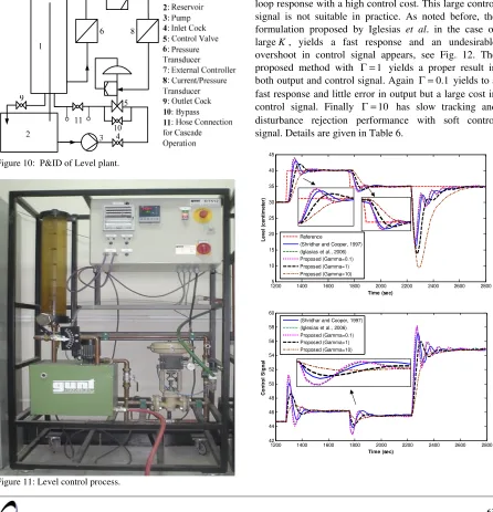
In this section, the proposed algorithm is implemented experimentally. The considered plant is a lab-scale water tank system. The structure of the plant is depicted in Fig. 10 and the real plant is given in Fig.11.

The control goal in this system is water level control in tank 1. Hand valve 8 determines the flow of outlet stream from the bottom of the main tank. A big reservoir tank 2 gathers outlet water and a pump 3 circulates the water. Flow of the pumped water is controlled by a control valve 5. This water pours to the main tank. A Level sensor measures the level of water in the main tank. Controller 6 should observe this measurement and apply appropriate command to the control valve.

Figure 10: P&ID of Level plant.

Figure 11: Level control process.

The plant output range is 0 to 60 centimeters. The linear operating range is 30 to 45 centimeters. First, FOPDT model of the system is achieved by step responses as,

(31)

( )

1 80

5 8

+ =

−

s e s G

s

Control objectives are both set point tracking and disturbance rejection. So, a set point change from 30cm to 40cm in 1280sec, 40cm to 35cm in 1760sec and a disturbance in 2232sec are considered. The disturbance is change in the outlet cock. In Table1 all tuning parameters of controller for this plant can be found. Figure 12 shows the results of the DMC tuning methods.

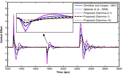
According to Fig. 12, it is shown that the tuning method developed by Shridhar and Cooper, yields a fast closed loop response with a high control cost. This large control signal is not suitable in practice. As noted before, the formulation proposed by Iglesias et al. in the case of largeK, yields a fast response and an undesirable overshoot in control signal appears, see Fig. 12. The proposed method with Γ=1 yields a proper result in both output and control signal. Again Γ=0.1 yields to a fast response and little error in output but a large cost in control signal. Finally Γ=10 has slow tracking and disturbance rejection performance with soft control signal. Details are given in Table 6.

12005 1400 1600 1800 2000 2200 2400 2600 2800 10

15 20 25 30 35 40 45

Time (sec)

L

e

v

e

l

(c

e

n

ti

m

e

te

r)

Reference

(Shridhar and Cooper, 1997) (Iglasias et al., 2006) Proposed (Gamma=0.1) Proposed (Gamma=1) Proposed (Gamma=10)

1200 1400 1600 1800 2000 2200 2400 2600 2800

42 44 46 48 50 52 54 56 58 60

Time (sec)

C

o

n

tr

o

l

S

ig

n

a

l

1200 1400 1600 1800 2000 2200 2400 2600 2800 -3

-2 -1 0 1 2 3 4 5 6 7

Time (sec)

C

o

n

tr

o

l

E

ff

o

rt

(Shridhar and Cooper, 1997) (Iglesias et al., 2006) Proposed (Gamma=0.1) Proposed (Gamma=1) Proposed (Gamma=10)

Figure 12: Experimental test results on Level plant.

TABLE 6

PERFORMANCE COMPARISON OF DMCTUNING METHODS,CASE

STUDY2.

Method Method of [8]

Method

of [10] Proposed Method

Γ - - 0.1 1 10

s

T 8 8 8 8 8

P 40 40 40 40 40

N 80 80 80 80 80

M 4 4 4 4 4

λ 7.1 3.17 2.65 21.14 168.7

IAE 283.3 257.9 251.8 372.6 616.1 2

u 9.778e+3 9.785e+3 9.789e+3 9.761e+6 9.725e+3 ∆ 2

u 38.94 52.1 54.78 25.38 14.52

TS 247 202 251.7 162 285

OV in u 398 430 307 170 63.6

OV in y 28.7 34 33.8 19.8 6.8 6. CONCLUSIONS

A new tuning method is proposed for DMC. Using FOPDT as the system model, an analytically function of FOPDT parameters is obtained via ANOVA and nonlinear regression. This leads to a closed form formula for tuning the DMC parameter. This parameter,λ, determines the quality of closed loop responses. Simulation and experimental case studies demonstrate the effectiveness of the proposed method in comparison with the other two available tuning methods.

7. REFERENCES

[1] SJ. Qin and TA, Badgwell, "A survey of industrial model predictive control technology," Control engineering practice, vol. 11, pp. 733-764, 2003.

[2] C. R. Cutler and B. L. Ramaker, "Dynamic Matrix Control: A Computer Control Algorithm," Proceeding of Joint Automatic Control Conference, 1980.

[3] E. F. Camacho and C. Bordons, Model Predictive Control, 2nd ed, Springer, 2005.

[4] W. Wojsznis, J. Gudaz, T. Blevins and A. Mehta, "Practical approach to tuning MPC," ISA Transactions, vol. 42, pp. 149-162, 2003.

[5] E. Ali and A. G. Ashraf, "On-line Tuning of Model Predictive Controllers Using Fuzzy Logic," The Canadian Journal of Chemical Engineering, vol. 81, pp. 1-11, Oct 2003.

[6] A. Jiang and A. Jutan, "Response Surface Tuning Methods in Dynamic Matrix Control of a Pressure Tank System," Ind. Eng. Chem. Res., vol. 39, pp. 3835-3843, 2000.

[7] A. R. Neshasteriz, A. Khaki Sedigh and H. Sadjadian, "Generalized predictive control and tuning of industrial processes with second order plus dead time models," Journal of Process Control, vol. 20, pp. 36-72, Jan 2010.

[8] R. Shridhar and D. J. Cooper, "A Tuning Strategy for Unconstrained SISO Model Predictive Control," Ind. Eng. Chem. Res, vol. 36, pp. 729-746, 1997.

[9] J. H. Lee, and Yu, Z.H, "Tuning of model predictive controllers for robust performance," Computer. Chem. Eng., vol. 18, pp. 15– 37, 1994.

[10] E. J. Iglesias, M. E, Sanjuán and C. A. Smith, "Tuning equation for dynamic matrix control in SISO loops," Ingeniería y Desarrollo, Issue 19, pp. 88-100, 2006.

[11] A. R. Neshasteriz, A, Khaki-Sedigh and H, Sadjadian, "An Analysis of Variance Approach to Tuning of Generalized Predictive Controllers for Second Order plus Dead Time Models," 8th IEEE International Conference on Control & Automation, 2009.

[12] L. Garriga and M. Soroush, "Model Predictive Control Tuning Methods: A Review," Ind. Eng. Chem. Res., vol. 49, pp. 3505– 3515, 2010.

[13] R. V. Hogg and J. Ledolter, Engineering statistics, MacMillan, 1987.

[14] H. Scheffe, The Analysis of Variance, New York: Wiley, 1959. [15] R. A. Fisher, Statistical methods for research workers, Oliver and

Boyd, Edinburgh, 1925.

[16] R. A. Fisher, The design of experiments, Oliver and Boyd, Edinburgh, 1935.

[17] A. M. Mora, J. J. Merelo, P. A. Castillo, J. L. J. Laredo and C. Cotta, "Influence of parameters on the performance of a MOACO algorithm for solving the bi-criteria military path-finding problem," Proceedings of the IEEE Congress on Evolutionary Computation, pp. 3507-3514, 2008.

[18] V. A. Niskanen, "Prospects for integrating analysis of variance with soft computing," Information Sciences, vol. 134, pp. 135-166, 2001.

[19] K. Barbe, W. Van Moer and Y. Rolain, "Using ANOVA in a Microwave Round-Robin Comparison," IEEE Transaction on Instrument, vol. 58, pp. 3490-3498, Oct 2009.

[20] J. A. D. Rodrigues, E. C. V. Toledo and R. M. Filho, "A tuned approach of the predictive-adaptive GPC controller applied to a fed-batch bioreactor using complete factorial design," Computers and Chemical Engineering, vol. 26, pp. 1493-1500, 2002. [21] R. S. Bogartz, An introduction to the analysis of variance, Praeger,

Connecticut, 1994.

[22] M. Henson and D. Seborg, "Adaptive nonlinear control of a pH neutralization process," IEEE Trans. Control Syst. Technol., vol. 2, pp. 169–182, 1994.

[23] J. Nie, A. P. Loh, and C. C. Hang, "Modeling pH neutralization process using fuzzy-neural approaches," Journal of fuzzy sets and systems, vol. 78, pp. 5-22, 1996.