Numerical solution of linear control systems using interpolation
scal-ing functions
Behzad Nemati Saray∗
Young Researchers and Elite Clube, Marand Branch, Islamic Azad University, Marand, Iran.
E-mail: [email protected]
Mohammad Shahriari
Department of Mathematics, Faculty of Science, University of Maragheh, Maragheh, Iran. E-mail: [email protected]
Abstract The current paper proposes a technique for the numerical solution of linear control systems. The method is based on Galerkin method, which uses the interpolating scaling functions. For a highly accurate connection between functions and their derivatives, an operational matrix for the derivatives is established to reduce the problem to a set of algebraic equations. Several test problems are given, and the numerical results are reported to show the accuracy and efficiency of this method.
Keywords. Linear control systems, Galerkin method, Interpolating scaling functions, operational matrix.
2010 Mathematics Subject Classification. 37L65 , 49N05, 65T60.
1. Introduction
The main purpose of this manuscript is to study numerical method based on in-terpolating scaling functions for the solution of the following linear optimal control problem (OCP)
˙
x=Ax(t) +Bu(t), x(t0) =x0,
J= 1 2x(tf)
TSx(t f) +
1 2
Z tf
t0
xTP x+ 2xTQu+uTRu
dt, (1.1)
wherex∈Rn,u∈
Rm,A∈Rn×n and B∈Rm×n. The controlu(t) is an admissible
control if it is piecewise continuous in t for t ∈ [t0, tf]. These values belong to a
given closed subsetU of R+. The input u(t) is derived by minimizing the quadratic
performance index J, where S ∈ Rn×n, P ∈ Rn×n and Q ∈ Rn×m are positive
semi-definite matrices andR∈Rm×m is positive definite matrix.
Optimal control theory are encountered in various fields such as engineering, eco-nomics, aerospace, chemical engineering, robotic and finance. We know, it is difficult to solve generally optimal control problems. Thus, the key to solve many of these real
Received: 29 August 2016 ; Accepted: 12 December 2016.
∗Corresponding author.
world problems are numerical methods. In order to solve linear quadratic OCPs, var-ious numerical approaches are proposed by researchers. Yousefi et al. presented the He’s variational iteration method [23] for the linear optimal control problem. Also see [7] for the use of the Adomian decomposition method for solving this equation. In [5], homotopy perturbation method was applied to solve optimal control problems. Also some other methods are used for solving this problem to transform the new problem such as converting the problem to differential inclusion form [11], or measure space and then solved in [4], genetic algorithm, and Others deal with the optimal control problem directly. For example see [6,8, 9,10,16,20,22] and the references therein.
Over the last decade, wavelets have found applications in numerous areas of math-ematics, engineering, computer science, statistics, physics, etc [19]. Multiwavelets are revealed to possess several advantages with respect to scalar wavelets. The reason of their success is due to the fact that, unlike scalar wavelets, multiwavelets can be constructed with several simultaneous properties, such as orthogonality, symmetry, having high numbers of vanish moments and closed form [18, 17]. In this work, we use the interpolating scaling functions which are introduced by Alpert [1,2]. In ad-dition to the simultaneous properties which proposed for multiwavelets, interpolating scaling functions have interpolating property. This feature reduces the time and com-putation cost. Also operational matrix of derivative is derived in [14,3] helps to save computing time. So, we use the interpolating scaling functions to solve Eq. (1.1). The outline of this paper is as follows. In Section 2, we describe the basic formulation of the interpolating scaling functions required for our subsequent development. In Sec-tion 3 the proposed method is used to approximate the soluSec-tion of the problem. As a result a set of algebraic equations are formed and a solution of the considered problem is introduced. In Section 4, we report our numerical findings and demonstrate the accuracy of the proposed numerical scheme.
2. The interpolating scaling functions
Suppose Pr be the Legendre polynomial of order r where r is a fixed
nonnega-tive integer number, and let τk for k = 0,· · ·, r−1 denote the roots of Pr. The
interpolating scaling functions (ISF) are given by [14]
φk(t) := ( q
2
ωkLk(2t−1), t∈[0,1], 0, otherwise,
whereωk are the Gauss–Legendre quadrature weights given as
ωk =
2 rP0
r(τk)Pr−1(τk)
,
andLk(t) are the Lagrange interpolating polynomials given as [15]
Lk(t) = r−1
Y
i=0, i6=k
t−τ
i
τk−τi
fork = 0,· · · , r−1. Now we can expand any polynomialsg on [0,1) of degree less thanr by using the functionsφ0,· · ·, φr−1 as
g(t) =
r−1
X
k=0
dkφk(t),
where the coefficientsdk are given by
dk =
r ωk
2 g τˆk), k= 0,· · ·, r−1,
where
ˆ τk=
τk+ 1
2 . Let
φknl(t) := 2
n
2φk(2nt−l), k= 0,· · ·, r−1, l= 0,· · · ,2n−1, (2.1)
wherenis a fixed nonnegative integer number, then we have the following orthonor-mality conditions [14]
Z 1
0
φknl(t)φ ´ k
n´l(t)dt=δl´lδkk´, k,k´= 0,· · ·, r−1, l,´l= 0,· · · ,2 n
−1.
2.1. The function approximation. For any two fixed nonnegative integer numbers randn, the functionf(t)∈L2[0,1] represented by ISF expansion as
f(t)≈
r−1
X
k=0 2n−1
X
l=0
sknlφknl(t) =STΦ(t), (2.2)
where
S =
s0n0, . . . , srn−10 |s0 n1, . . . , s
r−1 n1 |. . .|s
0
n,2n−1, . . . , srn,−12n−1]T, (2.3) Φ(t) =φ0n0(t), . . . , φ
r−1 n0 (t)|φ
0
n1(t), . . . , φ r−1
n1 (t)|. . .|φ 0
n,2n−1(t), . . . , φrn,−12n−1(t)]
T
,
and the coefficientsck
nlare computed as
sknl= Z 1
0
f(t)φknl(t)dt= Z hl+1
hl
f(t)φknl(t)dt,
where
hl=
l
2n, l= 0,· · ·,2 n−1.
These coefficients are computed by using Gauss-Legendre quadrature as
sknl= 2−n/2 r
ωk
2 f(2
−n(ˆτ
k+l)), k= 0, . . . , r−1, l= 0, . . . ,2n−1. (2.4)
Also the functiong(x, t)∈L2([0,1]×[0,1]), represented by ISF expansion as
g(x, t)≈
N
X
i=1 N
X
j=1
where G is anN×N matrix as
G=
g11 · · · g1N
..
. ...
gN1 · · · gN N
,
whereN =r2n and
gi,j=
Z 1
0
Z 1
0
g(x, t)Φi(t)Φj(x)dtdx, i, j= 1,2, . . . , N,
so that, by applyeing the method of [14] we get
gi,j= 2−n
r ωk
2 r
ωk0
2 g 2
−n(ˆτ
k+l),2−n(ˆτk0+l0), (2.6)
wherel=i−kr−1 andl0 =j−kr0−1,k, k0 = 0,1,· · ·, r−1.
2.2. The operational matrix of the derivative. Suppose that the derivative of f(t) in (2.2) given by
d dtf(t) =
r−1
X
k=0 2n−1
X
l=0
˜
sknlφknl(t) = ˜STΦ(t), (2.7)
where ˜S is a vector defined similarly to (2.3). We obtain the relation betweenS and ˜
S by
˜
S=DS, (2.8)
whereDis the operational matrix of the derivatives [12] for the ISFs. Using Eq. (2.7) we get ˜sk
nlas
˜ sknl=
Z hl+1 hl
φknl(t) d
dtf(t)
dt, k= 0, . . . , r−1, l= 0, . . . ,2n−1.
By integration by parts from the above integral, we get
˜ sknl=
f(t)φknl(t)hl+1 hl −
Z hl+1
hl f(t) d dtφ k nl(t) dt.
Using (2.1) and (2.2), we get
˜
sknl= 2(n/2)
f(hl+1)φk(1)−f(hl)φk(0)−2n r−1
X
i=0
qkisinl, (2.9)
where
qki=
Z 1
0
φi(t)
d dtφ
k(t)
dt, k, i= 0,1,· · ·, r−1.
Employing the Gauss-Legendre quadrature formula, we obtain
qki=
r ωi
2 d dtφ
k(ˆτ
To evaluatef(hl) andf(hl+1) we use the average of left and right limits onhl as
f(hl) =
1 2
r−1
X
i=0
sin,l−1φin,l−1(hl) + r−1
X
i=0
sinlφinl(hl)
!
, l= 1,· · ·,2n−1.
(2.10)
Using (2.1), we can express Eq. (2.10) as
f(hl) = 2
n 21 2 r−1 X i=0
sin,l−1φi(1) +
r−1
X
i=0
sinlφi(0) !
, l= 1,· · ·,2n−1. (2.11)
Also, to evaluate the values of functionf at the pointsh0 andh2n we have
f(h0) = r−1
X
i=0
sin0φin0(h0) = 2
n
2 r−1
X
i=0
sin0φi(0), (2.12)
f(h2n) =
r−1
X
i=0
sin,2n−1φin,2n−1(h2n) = 2 n
2 r−1
X
i=0
sin,2n−1φi(1). (2.13)
Substituting (2.11)–(2.13) in Eq. (2.9), we obtain
˜ skn0= 2n
"r−1
X
i=0
1 2φ
i(1)φk(1)
−φi(0)φk(0)−qki
sin0+
r−1
X
i=0
1 2φ
i(0)φk(1)si n1
# ,
˜ sknl= 2n
"r−1
X
i=0
−1
2φ
i(1)φk(0)
sin,l−1+
r−1
X
i=0
1 2φ
i(1)φk(1)
−1 2φ
i(0)φk(0)
−qki
sinl
+ r−1 X i=0 1 2φ
i(0)φk(1)si n,l+1
#
, l= 0,· · ·,2n−2,
˜
skn,2n−1= 2n "r−1
X
i−0
−1 2φ
i(1)φk(0)si
n,2n−2+
r−1
X
i=0
φi(1)φk(1)−1 2φ
i(0)φk(0)
−qki
sin,2n−1
# .
From the above equations, the matrix D can be expressed as a block tridiagonal matrix as
D= 2n R H
−HT R H
. .. . .. . .. . .. . .. . ..
−HT R H
−HT R
where, each block is anr×rmatrix and fork, i= 1, ..., r, we have
[R]ki= 1 2φ
i(1)φk(1)−φi(0)φk(0)−q ki,
[R]ki= 1 2φ
i(1)φk(1)−1
2φ
i(0)φk(0)−q ki,
Rki=φi(1)φk(1)−1 2φ
i(0)φk(0)−q ki,
[H]ki= 1 2φ
i(0)φk(1).
Since Eqs. (2.9)–(2.13) are exact for polynomials up to degreer−1 so the operational matrix of the derivative is exact for polynomials up to degreer−1.
3. Description of the numerical methods
Let us begin to solve the following linear optimal control problem (OCP). For this purpose, we consider Pontryagin’s maximum principle (P M P) for system (1.1) and achieve the optimal control lawu∗(t) =−k(t)x(t). According to theP M P, one has
˙
λ=−∂H
∂x =−P x−Qu−A
Tλ, (3.1)
∂H ∂u =Q
Tx+Ru+BTλ= 0, (3.2)
where H is Hamiltonian of the system (1.1), so
H(x, u, λ, t) = 1 2 x
TP x+ 2xTQu+uTRu
+λT(Ax+Bu), (3.3)
alsoλ∈Rn is co-state vector. The optimal control is computed by
u∗=−R−1QTx−R−1BTλ, (3.4)
whereλandxare the solution of the following Hamiltonian system
x˙ = [A
−BR−1QT]x−BR−1BTλ,
˙
λ= [−P+QR−1QT]x+ [QR−1BT −AT]λ, (3.5)
with the initial conditionx(t0) =x0 and the terminal conditionλ(tf) =Sx(tf) [13].
This system of equation is linear, so we obtain
x λ
=
F(t, tf) G(t, tf)
L(t, tf) M(t, tf)
x(tf)
λ(tf)
, (3.6)
whereF,G, LandM aren×nmatrices. Applying the terminal condition and so
x(t) = (F+GS)x(tf),
λ(t) = (L+M S)x(tf).
(3.7)
IfF+GSis invertible, we get
λ(t) = (L+M S)(F+GS)−1 | {z }
Y(t,tf)
After differentiating with respect to thet from Eq.(3.8), we have
˙
λ(t) = ˙Y(t, tf)x(t) +Y(t, tf) ˙x(t). (3.9)
Using equations (3.5) and (3.8) from [13], one can write
˙
Y = (Y B+Q)R−1(BTY +QT)−Y A−ATY −P, (3.10)
also by applying the optimal control law (3.4), we have
u∗(t) =−R−1QTx−R−1BTY(t, tf)x(t). (3.11)
According to equation (3.8) the terminal conditions for equation (3.10) are
F(tf, tf) =I, G(tf, tf) = 0,
L(tf, tf) = 0, M(tf, tf) =I.
(3.12)
By considering the following variables
V(t) =F(t, tf) +G(t, tf)S,
W(t) =L(t, tf) +M(t, tf)S,
(3.13)
and substituting these new variables into (3.7) and then into (3.5), one has
˙
V(t) = A−BR−1QTV(t)−BR−1BTW(t), ˙
W(t) = −P+QR−1QT
V(t) + QR−1BT −AT
W(t), (3.14)
with conditionsV(tf) =I andW(tf) =S.
Assume that we expandV(t) andW(t) using interpolating scaling functions as
V(t)≈VΦ(t),
W(t)≈WΦ(t), (3.15)
whereVandWare the (n×N) unknown vector. By differentiating from both sides of Eq. (3.15), and using Eq. (2.10), we get
˙
V(t)≈VDΦ(t), ˙
W(t)≈WDΦ(t). (3.16)
Now replacing (3.15) and (3.16) in (3.14) yields
VD− A−BR−1QT
V+BR−1BTW
Φ(t) = 0,
VD− −P+QR−1QT
V− QR−1BT −AT W
Φ(t) = 0. (3.17)
The entries of vector Φ(t) are independent, so we obtain
VD− A−BR−1QT
V+BR−1BTW= 0,
VD− −P+QR−1QT
V− QR−1BT−AT
W= 0, (3.18)
4. Numerical Experiments
In this section, some numerical examples are presented to illustrate the validity and the merits of the new technique. We reportl∞error of the solution that is defined as
L∞= max
0≤i≤10|ui−u˜i|,
where ui and ˜ui are the exact and computed values of the solution u at the points
ti= 10i, i= 0,1,· · ·,10, respectively.
Example 4.1. Consider a single-input scalar system as follows:
˙
x=−x(t) +u(t),
J= 1/2 Z 1
0
(x2(t) +u2(t))dt, (4.1)
with initial condition
x(0) = 1. (4.2)
The exact solution of this problem is [13]
x(t) = cosh(√2t) +βsinh(√2t),
u(t) = (1 +√2β) cosh(√2t) + (√2 +β) sinh(√2t),
where
β=−cosh( √
2t) +√2 sinh(√2t) √
2 cosh(√2t) + sinh(√2t).
After using the method proposed in the previous section, we obtain
˙
V(t) =−V(t)−W(t), ˙
W(t) =−V(t) +W(t), V(0) = 1, W(1) = 0,
where, the following optimal control law may be computed by
u∗(t) =−W(t).
Table 1,2 consist of L∞ norm of example 1 forN ={6,8}. Figure 1 shows the plot
of approximate solutions of Eq (4.1) also Figure 2 demonstrates the plot of absolute errors.
Table 1. L∞ error ofx(t) for various values of N for Example (4.1).
t 0 0.2 0.4 0.6 0.8 1
N = 6 0 4.68e-6 3.62e-6 3.05e-6 2.77e-6 2.32e-6
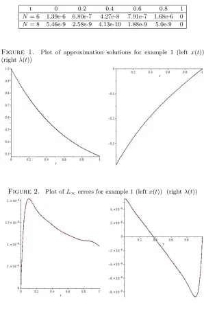
Table 2. L∞ error ofλ(t) for various values of N for Example (4.1).
t 0 0.2 0.4 0.6 0.8 1
N= 6 1.39e-6 6.80e-7 4.27e-8 7.91e-7 1.68e-6 0
N= 8 5.46e-9 2.58e-9 4.13e-10 1.88e-9 5.0e-9 0
Figure 1. Plot of approximation solutions for example 1 (left x(t)) (rightλ(t))
Figure 2. Plot ofL∞errors for example 1 (leftx(t)) (rightλ(t))
Example 4.2. Consider a single-input scalar system as follows:
˙
x(t) =u(t),
J = Z 1
0
with the initial condition
x(0) = 0. (4.4)
For this example, the analytical solutio is [21]
x(t) =e(e2(t−e2e−1)(−t)),
u(t) =e(e2(t+e2e−1)(−t)).
Therefore, we should have
˙
V(t) =−1 2W(t),
˙
W(t) =−2V(t), V(0) = 0, W(1) = 0.
Also, we can obtain the following optimal control law
u∗(t) =−W/2,
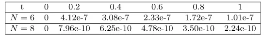
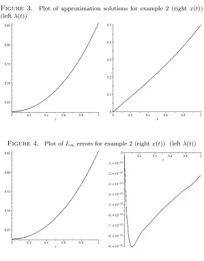
Table 3,4 consist of L∞ norm of example 2 forN ={6,8}. Figure 3 shows the plot
of approximate solutions of Eq (4.3) also Figure 4 demonstrates the plot of absolute errors.
Table 3. L∞ error ofx(t) for various values of N for Example (4.3).
t 0 0.2 0.4 0.6 0.8 1
N= 6 0 4.12e-7 3.08e-7 2.33e-7 1.72e-7 1.01e-7
N= 8 0 7.96e-10 6.25e-10 4.78e-10 3.50e-10 2.24e-10
Table 4. L∞ error ofλ(t) for various values of N for Example (4.3).
t 0 0.2 0.4 0.6 0.8 1
N = 6 5.37e-7 4.78e-7 4.05e-7 3.50e-7 3.19e-6 0 N = 8 1.07e-9 9.29e-10 7.88e-10 6.79e-10 5.97e-10 0
5. Conclusion
Figure 3. Plot of approximation solutions for example 2 (right x(t)) (leftλ(t))
Figure 4. Plot ofL∞errors for example 2 (rightx(t)) (leftλ(t))
Acknowledgment
This work was supported by the Young Researchers and Elite Clube, Marand Branch, Islamic Azad University, Marand, Iran [grant number 94171 ]. We would like to thank one of the referees for his comments.
References
[1] B. Alpert, G. Beylkin, D. Gines, L. Vozovoi, Adaptive solution of partial differential equations in multiwavelet bases, J. Comput. Phys., 182 (2002), 149–190.
[2] B. Alpert, G. Beylkin, R. R. Coifman, V. Rokhlin, Wavelet–like bases for the fast solution of second–kind integral equations, SIAM J. Sci. Statist. Comput., 14 (1993), 159–184.
[4] S. Effati, M. Janfada and M. Esmaeili, Solving the optimal control problem of the parabolic PDEs in exploitation of Oil, Journal of Mathematical Analysis and Applications, 340(1) (2008), 606–620.
[5] S. Effati, H. Saberi Nik. Solving a class of linear and nonlinear optimal control problems by homotopy perturbation method. IMA J. Math. Control Inform. 28(4) (2011), 539–553. [6] G. N. Elnagar, State-control spectral Chebyshev parameterization for linearly constrained
qua-dratic optimal control problems, Computational Applied Mathematics, 79(1) (1997), 19–40. [7] A. Fakharian, M.T. Hamidi Beheshti, A. Davari, Solving the b HamiltonJacobiBellman equation
using Adomian decomposition method. Int. J. Comput. Math., 87 (2010), 2769–2785.
[8] O. S. Fard and H. A. Borzabadi, Optimal control problem, Quasi-assignment problem and genetic algorithm, Proceedings of World Academy of Science, Engineering and Technology, 21 (2007), 70–43.
[9] H. Hashemi Mehne and A. Hashemi Borzabadi, A numerical method for solving optimal control problem using state parametrization, Numerical Algorithms, 42(2) (2006), 165–169.
[10] H. P. Hua, Numerical solution of optimal control problems, Optimal Control Applications and Methods, 21(5) (2000), 233–241.
[11] A. V. Kamyad, M. Keyanpour and M. H. Farahi, A new approach for solving of optimal nonlinear control problems, Applied Mathematics and Computation, 187(2) (2007), 1461–1471.
[12] M. Lakestani, M. Dehghan, Numerical solution of Riccati equation using the cubic B–spline scaling functions and Chebyshev cardinal functions, Computer Physics Communications, 181 (2010), 957–966.
[13] H. Saberi Nik. S. Effati. A. Yildirim, Solution of linear optimal control systems by differential transform method, Neural Comput and Applic, 23 (2013), 1311-1317.
[14] M. Shamsi, M. Razzaghi. Numerical solution of the controlled duffing oscillator by the interpo-lating scaling functions, Electrmagn. Waves and Appl, 18(5) (2004), 691–705.
[15] M. Shamsi, M. Razzaghi, Solution of Hallen’s integral equation using multiwavelets, Comput. Phys. Comm., 168 (2005), 187–197.
[16] H. R. Sirsena and K. S. Tan, Computation of constrained optimal controls using parameteriza-tion techniques, IEEE Transacparameteriza-tions on Automatic Control, 19(4) (1974), 431–433.
[17] G. Strang and V. Strela, Orthogonal multiwavelets with vanishing moments, OPT. ENG., 33(7) (1994), 2104-2107.
[18] V. Strela, P. N. Heller, G. Strang, P. Topiwala, and C. Heil, The application of multiwavelet filterbanks to image processing, IEEE T. IMAGE PROCESS, 8(4) (1999), 548-563.
[19] W. Sweldens, The Lifting Scheme: A Construction of Second Generation Wavelets, SIAM J. Math. Anal., 29(2) (1998), 511-546.
[20] K. L. Teo, C. J. Goh and K. H. Wong, A unified computational approach to optimal control problem, Longman Scientific and Technical, Harlow, 1991.
[21] E. Tohidi, H. Saberi Nik, A Bessel collocation method for solving fractional optimal control problems, Applied Mathematical Modelling, 39 (2015), 455-465.
[22] J. Vlassenbroeck and R. V. Dooren, A Chebyshev technique for solving nonlinear optimal control problems, IEEE Transactions on Automatic Control, 33(4) (1998), 333-340.