Vol 3, No. 2, (2013), pp 67-77
Relation between intersection of
nullclines and periodic solutions in a
differential equations of p53 oscillator
F. Rangi and M. Tavakoli
Abstract
We consider a simple mathematical model that suggests emergence of oscillations in p53 and Mdm2 protein levels in response to stress signal. In-tracellular activity of the p53 protein is regulated by a transcriptional target, Mdm2, through a feedback loop. The model is classified in five cases with respect to intersection of nullclines. In each case occurrence(or not) of the limit cycle is investigated.
Keywords: DNA damage; p53-Mdm2; Limit cycle; Mathematical biology.
1 Introduction
The p53 protein is suppressor tumor that plays an important role in growth, arrest, senescence, and apoptosis in response to broad array of cellular dam-age.In more than 50% of human cancer, the p53 is muteted[3]. Under normal, unstressed conditions (for example calls dont suffer DNA damage or no DNA damage) the concentration of p53 is kept at low levels by Mdm2 gene. Mdm2 plays a key role in preserving p53 levels low in normal cell while the Mdm2 transcription is induced by p53 itself[3]. Thus with negative feedback loop (p53 →M dm2 ⊣ p53) any increase of p53 normally leads to an increase in Mdm2 levels, which then pushes p53 back down to a low steady state level[7]. But In environmental stresses such as DNA damage, the concentration of p53 increase and inducing a transition to oscillations of p53 level [4]. Namely p53 arrests the cell cycle, thereby giving the cell time to correct any DNA dam-age, activates transcription of genes which is indirectly responsible to DNA repair, and can be the cause of apoptosis [2]
Lahava et al. in [8] measured intercellular concentration of total p53 and Mdm2 protein and observed p53 and Mdm2 protein concentration in a
Recieved 19 February 2013; accepted 12 June 2013 Fahimeh Rangi
Department of Applied Mathematics, Ferdowsi University of Mashhad, Mashhad, Iran, e-mail: f [email protected]
Mahboobeh Tavakoli
Pardis of Hasheminejad, Farhangian University, Mashhad, Iran. e-mail: [email protected]
single cell oscillation in response to DNA damage, and proposed that system behaved as a digital oscillator [2].
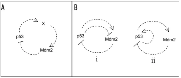
The generation of oscillations in the p53/Mdm2 network seems a chal-lenge to modellers, becuase negative feedback is not sufficient for oscillatory behaviors. For example, a negative feedback composed of only two elements, such as p53 → M dm2 ⊣ p53, cannot oscillate. The observation of Lahava et al. in [8] leads to several interesting model and hypotheses [3, 9]. In fact several mathematical models have been proposed to explain the damped os-cillations of p53, either in cell population or in a single cell, most of which are deterministic models of ordinary differential equations [15]. Lev Bar Or et al. considered the possibility of a negative feedback loop composed of three components (Mdm2, p53 and putative intermediate factor), which can oscillate (part A of Figure1) or require the simultaneous presence of negative and positive feedbacks (part B of Figure1)[3] .
Figure 1: Pathways to oscillations. Oscillation can be found in two different types (A) negative feedback loops with three or more components and (B) combinations of negative and positive feedbacks
Tysonin response the observation ofLahavawhich showed the digital os-cillator behavior, assumed the steady state p53 concentration passes through a hopf bifurcation in following DNA damage and the p53 and Mdm2 levels begin to oscillate [2, 15]. In [2]another protein (The Atm protein) has been mentioned that is similar to a switch that caused the p53- Mdm2 oscillator be into or out to oscillatory zone. By following to in[12] regions of parameters into which the Atm protein can switch off damage signals, are determined.
Another approach to modeling the p53 dynamics make explicit use of delays in the system corresponding to the time that it takes for transcription and translation of proteins [10, 14, 16].
A recent elementary model which is motivated biologically according to case ii in part B of Figure1 (autocatalysis) formulates as below
˙
x= α0+
α1xn
k1+xn −
γ1xy−γ2x=F
˙
y= α2+
α3x4
k2+x4 −
γ3y=G
(1)
where x(t) = [p53(t)] and y(t) = [M dm2](t) are denoting concentration of p53 and Mdm2 respictively[2]. In the first equation above,α0 shows the
production rate of p53, the second therm with coefficient α1 represents an
autocatalytic process and it is described with a Hill coefficient n∈N which determines the degree of cooperativity of the ligand of p53 binding to the enzyme or receptor [5]. The third therm represents the active process of ubiquitination of p53 independently of Mdm2 and the fourth term represents the degradation of p53 independently of Mdm2. Similarly in the second equation above,α2shows the production rate of Mdm2, and second term with
coefficientα3represents the activation of Mdm2 by p53 whit Hill coefficient
4, and the third represents the degradation of Mdm2 [2] .
Analysis the trace and determinate of system (1) can be shown in addition to negative feedback loop in p53 - Mdm2 network, autocatalysis by either p53 or Mdm2 leads to the possibility of oscillatory behavior. In the absence of autocatalysis, one can still get oscillations if p53 also down-regulates Mdm2 or Mdm2 also up-regulates p53, in addition to the normal activation.
Here, Oscillatory behavior was described in the form of a limit cycle i.e. to obtain oscillatory behavior from each initial condition the fixed point of the system that resides within the limit cycle needs to be an unstable spiral. In this case all trajectories in the phase plane originating at near that fixed point spiral out and asymptote onto the limit cycle [2].
The goal of system biology is to analyze the behavior and interrelation-ships of functional biological system [13]. we analyze system (1) ) to find out the possible cases for existence of limit cycles that oscillatory behavior in p53-Mdm2 network is described. In fact the DNA damage can be controlled when slightly oscillatory region would be given in system (1). In other word, by changing the parameter values (parameter values to get the oscillation) and conditions are imposed on the system (1), then system has the stable limit cycle (oscillatory mode). Therefore, giving cell time to the repair the damage and will not develop cancer. For this purpose we use the Poincare Bendixson Theorem that possible case are shown for existence or nonexis-tence of limit cycle in system (1). The Poincare Bendixson theorem says that ast→ ∞the trajectories will tend to a limit cycle solution[11].
On of the most useful tools for analyzing nonlinear systems of differential equations (especially planer systems) are the nullclines. For a system in the form
˙
x1= f1(x1, x2,· · ·, xn) ..
. ˙
xn= fn(x1, x2,· · ·, xn)
(2)
Thexj -nullcline is the set of points where ˙xj vanishes, so the xj -nullcline is the set of points determined by settingfj(x1, x2,· · · , xn) = 0 [6].
First, with regard to the intersections of x- and y- nullcline (equilibrium point) of system (1), We classify them in several cases. In any of regions between the nullclines, the vector field is neither vertical nor horizontal, so it must point in one of four direction: northeast, northwest, southeast or southwest. We call such regions basic region[6]. The basic regions where
˙
x̸= 0 and ˙y̸= 0 are of four types:
A: ˙x >0,y >˙ 0 B: ˙x <0,y >˙ 0 C: ˙x <0,y <˙ 0 D: ˙x >0,y <˙ 0
Equivalently, these are the regions where the vector field points northeast, northwest, southwest, or southeast, respectively. [6].
Next we investigate the possibility of existence or nonexistence of limit cycles in system (1) by using Poincare Bendixson theorem. The Poincare Bendixson theorem says when the trajectory will tend to a limit cycle solution as t→ ∞.
2 Classifying of nullclines
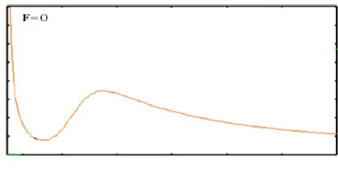
x- nullcline in system (1) is the set of points whereF(x, y) = 0.
F(x, y) = 0 =⇒y=f(x) = 1
γ1
(α0
x +
α1xn−1
k1+xn −
γ2) (3)
The mapy=f(x) has two critical point
x1,2= n
√
k1(−2α0+α1(n−1)± √q)
2(α0+α1)
(4)
where
q=−4nα0+α21n 2−2α2
1n+α 2
1 (5)
If we assume that x1 and x2 are positive, real and different; Therefore q
Figure 2: x-nullcline
So ifx→0, then f(x) =y → ∞. Since thex1 andx2 are positive and
x1 > x2 then sign f′ is negative in interval (0, x2) and the map y=f(x) is
decreases in this area. The sign off′ is changed inx2 becausex1 andx2 are
simple roots of equationy =f′(x). Therefore signf′ is positive betweenx1
and x2 and the map y=f(x) is increases in (x2, x1). The map has a change
of sign inx1, so sing f′ is negative in (x1,∞) andy =f(x) is decreasing in
this interval. Thereforex1and x2 are maximum and minimum fory=f(x)
, respectively.
Also, for the graph of G(x,y)=0 i.e. y - nullcline We have
G(x, y) = 0 =⇒y=g(x) = 1
γ3
( α3x
4
k2+x4
+α2) (6)
and
lim x→0g(x) =
α2
γ3
, lim
x→+∞g(x) =
α3
γ3
(7)
and
g′(x) = 1
γ3
( 4α2k2x3
(k4+x4)2
)
(8)
Sog′(x)>0 in the first region coordinate system (x >0, y >0). Therefore g(x) increases in this region
Now with regard to the intersections of x- and y- nullclines of system (1), it is classified in several cases and we obtained the vector field for each of these cases by XPP software. We discussed possibility of existence or nonexistence of limit cycle near the equilibrium point (intersection of nullclines).
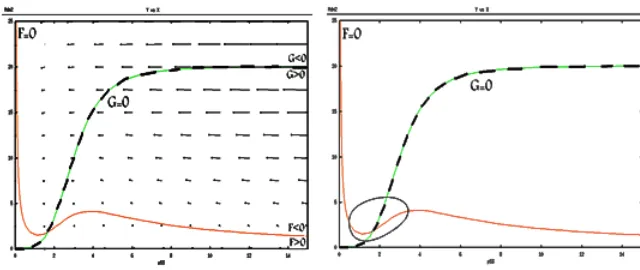
Case 1: The intersection before minimization
Figure 3: y-nullcline
to get the sing ofFyandFxandGxandGy for Jacobin matrix system(1) in intersection point .
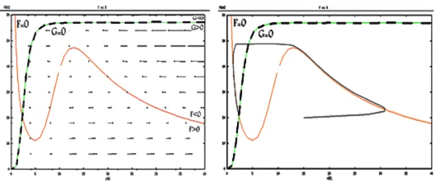
Figure 4: The vector field and nullclines and trajectory solution for the first case
A=
(
Fx(xs, ys) Fy(xs, ys)
Gx(xs, ys)Gy(xs, ys)
)
(9)
We move a long a line parallel to the x-axis through the equilibrium point , F decreases since F >0 the lower x-side andF <0 on the higher x-side. Therefore, Sign ofFxis negative. Similarly, we move a long a line parallel to they-axis through the equilibrium point ,Gdecreases sinceG >0 the lower
y-side andG <0 on the highery-side (for detail see [11]). Therefore, Sign of
dx
dy]F=0=− Fy
Fx
<0, Fx<0⇒Fy<0 (10)
dx dy
]
G=0
=−Gy
Gx
>0, Gy<0⇒Gx>0 (11)
In this case, sign of Jacobin matrix is equal
A=
(
− −
+−
)
(12)
Therefore trace of A matrix is negative and eigenvalues of A matrix is equal
λ1,2=
trA
2 ±
1 2
√
(trA)2−4detA (13)
The equilibrium point is stable since eigenvalue of system (1) is negative real part. Therefore system (1) by the Poincare Bendixson Theorem do not have limit cycle near the intersection point in this case.
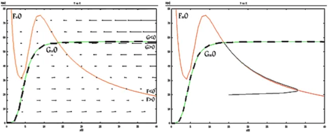
Case 2: the intersection after maximization of graph F=0
The vector field is plotted in Figure 5. By a similar process in the first case,
Figure 5: The vector field and nullclines and trajectory solution for the second case
the sign at A matrix is equal
A=
(
− −
+−
)
(14)
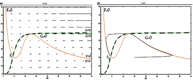
Case 3: the intersection between maximum and minimum of graph F=0
Figure 6 showes the vector field in this case. Similarly we have
Figure 6: The vector field and nullclines and trajectory solution for the third case
A=
(
+−
+−
)
(15)
In this case, it is possible that system (1) admits periodic solution [11]. We plotted the limit cycle near the intersection point in Figure 6 .
Case 4: two intersection points
We observe that system has two stable intersection points, whichS1 point is
similar to first case. So system (1) has not limit cycle near the intersection point in this case.
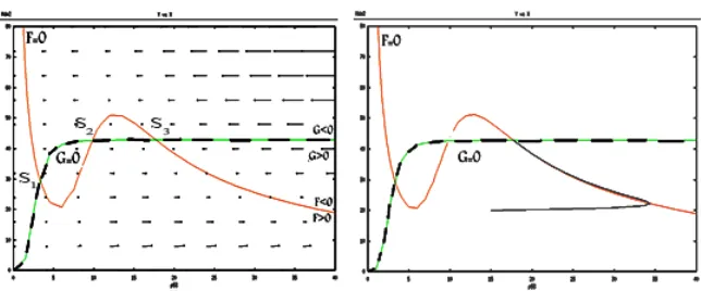
Case 5: three intersection points (after maximum, between max-imum and minmax-imum, before minmax-imum)
In Figure 8, S1 and S3 points are located before of x2 and after of x1
re-spectively. Thus system (1) don’t have limit cycle near these points, because
S1 andS2 are stable points.
ForS2 we have
Fx>0, Fy<0, Gx>0, Gy<0 (16)
0< dy dx
]
G=0
< dy dx
]
F=0⇒
0<−Gx Gy
<−Fx Fy
. (17)
So
Figure 7: The vector field and nullclines and trajectory solution for the fourth case
This shows that S2 is saddle point. According to the Poincare Bendixson
theorem, this type of singularity does not admit periodic solutions. For more details see([11]Section 7.3)
In following theorem we prove analytically that the only possible case for the existence of limit cycle is second case and other cases don’t have limit cycle at all.
Theorem 3. Theorem:System (1) can not admit limit cycle in cases 1, 2, 4 and 5 for the positive value ofγ1, γ3 andxs(intersection point of nullclines).
Proof. If (xs, ys) is equilibrium point of system (1) then Jocobian matrix of system (1) is equal
A=
(
Fx(xs, ys) Fy(xs, ys)
Gx(xs, ys)Gy(xs, ys)
)
(19)
and eigenvalues of matrix A are
λ1,2=
trA
2 ±
1 2
√
(trA)2−4detA (20)
By Gx=−Gy
dg
dx andFx=−Fy df
dx we have
det(A) =FxGy−FyGx=−FxGy
df
dx+FyGy dg
dx ⇒det(A) =FyGy(g
′−f′) (21) Also
Figure 8: The vector field and nullclines and trajectory solution for the fifth case
Then
λ1,2=
γ1xsf′(xs)−γ3±
√
(γ1xsf′(xs)−γ3)2−4γ1γ3xs(g′(xs)−f′(xs)) 2
(23) Now since the (x1, y1) point is maximum of mapf, if the intersection occurs
after maximum point thenf′(xi)≤0 for each ofxi thatxi≥x1 . Hence we
have f′(xs)≤0 , so by the positive value ofγ1, γ3 and xs,trA <0 and the (xs, ys) point is stable point. Therefore trajectory of solution limits to that point and we don’t have limit cycle near this point.
Similarly if the intersection of mapsf andg occurs before minimum of map
f then the trace of matrixAis negative because of we havef′≤0 in interval (0, x2] and so this point is a stable point that trajectory of system (1) limits
to that point.
References
1. Bar-Or, R. L., Maya, R., Segel, L. A., Alon, U., Levine, A. J. and Oren, M. Geneneration of oscillations by the p53-Mdm2 feedback loop:Atheorical and experimental study, Departements of Molecurlar Cell Biology and Applied Mathematics and Computer Scince, 97 (2000), 11250–11255.
2. Chicarmane,V., Ray,A., Sauro, H. M. and Nadim, A. A model for p53
3. Ciliberto, A., Novake, B. and Tyson, J.J.Steady States and Oscillations in the p53/Mdm2 NetworkCell Cycle 4:3. , 130 (2005), 488–493.
4. Ge H. and Qian, M. Boolean Network Approach to negative Feedback Loops of the p53Pathways: Synchronized Dynamics and stochatics Limit cycle, Jornal of computation biology, 6, 1 (2009), 119–132.
5. Hill, A. V. The possible effects of the aggregation of the molecules of hamoglobin on its dissosiation curves, J. Physiol., 40 (1910), 4–7.
6. Hirsch, M. W., Smale, S. and Devaney, R. L. Differntial equation , dy-namical systems and introduction to chaos, second edition, Elsevier, USA, 2004.
7. Lahva, G.Oscillations by the p53-Mdm2 feedback loop, Journal of Con-struction Engineering and Manage-ment, 131 (2005), 1115–1123.
8. Lahva, G., Rosenfeld, N., Sigal, A., Geva-Zatorsky, N., Levine, A.J., Elowitz, M. B. and Alon, U.Dynamics of the p53-Mdm2feedback loop in the individual cells, Nature Genetics, 36 (2004), 147–150.
9. Ma, L., Wangner, J., Rice, J. J., Hu, W., Levvien, A. J. and Storlovitzky, A.A plausible model for the digital response of p53 to DNA damage, Proc. Nat. Acad. Scien., 102 (2005), 14266–14271.
10. Monk, N. A. M. and Rice, J. J.Oscillatory expression of Her1, p53, and NF-kappaBdriven by transcriptional time delays, Current Biology, 97 (2000), 11250–11255.
11. Murray, J. D. Matematical Biology ,3rd edition, Springer-Verlag Berlin Heidelberg, 1991.
12. Rabiei motlagh, O. and Afsharnezhad, Z.On the conditions for which the Atm protein switch off the DNA damage signal in a p53 model, Studia Universitatis BAbes- Bolyal, Biologia, 1 (2010), 67–79.
13. Sauro, H., Adelinde, M., Uhrmacher, M., Harel, D., Hucka, M., Kwiatkowska, M., Mendes, P., Shaffer, C. A., Stromback, L. and Tyson, J. J. Challenges for modeling and simulation methods in systems biol-ogy,Proceedings of the 2006 Winter Simulation Conference, 67–79.
14. Tiana, G., Jensen, M. H. and Sneppen, K.Time delay as a key to opop-tosis induction in the p53 network, Euro. Phys. j., 39 (2002), 135–140.
15. Tyson, J. J.Monitoring p53’s pulse, Nature Genetics, 36 (2004), 113–114.