A peer-reviewed, open-access journal of population sciences
DEMOGRAPHIC RESEARCH
VOLUME 29, ARTICLE 23, PAGES 617-640
PUBLISHED 27 SEPTEMBER 2013
http://www.demographic-research.org/Volumes/Vol29/23/ DOI: 10.4054/DemRes.2013.29.23
Research Article
Age groups and the measure of population
aging
Hippolyte d’Albis
Fabrice Collard
c
2 Related literature 619
3 Endogenous age groups and the measurement of population aging 621
3.1 An example 622
3.2 Methodology 625
4 The dynamics of population aging in industrialized countries 628
4.1 Aging in the US 628
4.2 On the number of groups 631
4.3 An international perspective 633
5 Conclusion 635
6 Acknowledgements 636
References 637
Age groups and the measure of population aging
Hippolyte d’Albis1
Fabrice Collard2
Abstract
BACKGROUND
Measures of population aging are important because they shape our perception of demo-graphic trends. Indicators of aging based on fixed ages contributed to a dramatic portrayal of demographic evolutions, some of which were associated with the myth of decline.
OBJECTIVE
We propose a new measure of population aging, based on the relative age of each indi-vidual in the population. Our approach builds on previous work by Aghevli and Mehran (1981) and relies on optimal grouping techniques that are used to determine the various age groups within a population. The cutoff ages for these groups, such as the age from which an individual is considered to be an older person, are then endogenous variables that depend on the entire population age distribution at any given moment.
METHODS
We show how to apply optimal grouping techniques to age distributions and how to calcu-late various indicators of aging, which are invariant with respect to proportional rescaling of distributions. We compute these indicators for the US, and a sample of 13 other indus-trialized countries.
RESULTS
We find that, contrary to common arguments for an aging population, the share of elderly individuals within the total population has not increased much, and has remained stable in these countries. These results complement and reinforce the earlier findings of Sanderson and Scherbov (2005, 2007) who also reassessed the aging phenomenon.
1Correspondending author. Paris School of Economics, University Paris 1/ Centre d’Economie de la Sorbonne,
106 boulevard de l’Hôpital, 75013 Paris, France. E-mail: [email protected].
“The first part of life is childhood. The second is your child’s childhood. And then the third, old age.”Barbara Kingsolver,The Lacuna
1.
Introduction
Population aging is often perceived as a very widespread phenomenon. According to the last United Nations “Population Aging Report” (2009), the proportion of the global population aged over 60 years was 8% in 1950, 10% in 2000, and is expected to reach 21% in 2050. In this report, the United Nations have used a very specific, albeit very common, type of measurement for assessing the population aging phenomenon, namely the proportion of population aged over 60. And yet, it is evident that today’s 60-year-olds are often very different from their parents at the same age and have absolutely nothing in common with their grandparents at the same age. The age at which one becomes an older person is a notion that changes over time; thus, calculating the proportion of older persons based on a fixed age only provides us with biased information. The use of such an indicator is often justified on the ground that these fixed ages (60, 65 or 80, depending on the study) correspond to the eligibility ages of certain social programs, most notably the pay–as–you–go pension system. However, recent events, for example in Europe, show that these ages also undergo changes (see notably Fenge et al., 2008, and references therein). Indicators, though simple, are not neutral. While studying the history of social representation that defines old age as starting from 60 years, Bourdelais (1994, 1999) showed that indicators of aging based on fixed ages contributed to a dramatic portrayal of demographic evolutions, some of which were associated with the myth of decline. The aim of our paper is to propose a new means of determining the various age groups in a population and to recalculate new indicators of aging based on the cutoff ages of these groups.
direct implication of this grouping is that the definition of old age fundamentally relies on the relative position of each cohort in total population and thus depends on the entire shape of the age distribution. Our concept of the stages of life is a relative one: the “age” of individuals within a given cohort depends on the size of the other cohorts. This is a statistical interpretation of the what is nicely characterized by B. Kingsolver in the quotation we reproduced above.
Optimal grouping techniques were initially used by Aghevli and Mehran (1981) and Davies and Shorrocks (1989) for income distribution issues, and applied by Esteban et al. (2007) to polarization measurements. In this paper, we demonstrate in a formalized manner how to apply these techniques to age distributions in order to calculate cutoff ages. The latter then allow us to calculate various indicators of aging, which are invariant with respect to proportional rescaling of distributions. These calculations are no more complicated than those proposed in related contributions, which will be described below. Most notably, in the extreme case where only two age groups are considered, our indicator of aging becomes the proportion of individuals whose age is greater than the mean age.
Applying this technique to total US population, we find that the age at which one be-comes an older person has dramatically increased over the last century. In our benchmark experiment involving 4 age groups, we find that the entry age into oldness was 48.7 years in 1933 and skyrocketed to 57.6 years in 2005. Most industrialized countries exhibit the same behavior of the entry age into oldness. We then find that the share of the so-defined elderly in total population remained stable over time and does not display a pronounced upward sloping trend. We then compute the elder-child ratio and find that its time average increased over the last 50 years by less than 6.5% in the US, and by less than 8% on av-erage in a sample of 13 industrialized countries. These findings then suggest that aging is less pronounced when a measure that takes evolutions in the age distribution into account is used.
The remainder of the paper is organized as follows. Section 2 compares our method to recent contributions in the field. Section 3 describes our approach to defining endogenous age groups and defines our aging indicators. Section 4 revisits aging in the US and in 12 other industrialized countries in light of our new indicators. A last section offers some concluding remarks.
2.
Related literature
individual’s age not according to the number of years lived since birth, but according to the remaining number of years that he or she is expected to live. Thus, Ryder proposes considering an individual as an older person when his or her remaining life expectancy is less than ten years. This type of characterization, which may be used to define the proportion of older persons in a population, constitutes a major advancement, as it enables the distinction between individual and population aging. This idea has been pursued by Sanderson and Scherbov (2005, 2010), who establish the mean age of an age pyramid that is recalculated based on the life expectancy at each age.
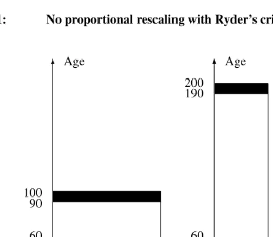
However, such approaches have two drawbacks. First, at a given date, a cohort’s life expectancy is unknown and its estimation using a period life table is imperfect (Goldstein and Wachter, 2006), although the approximation error is likely to be quantitatively small (Sanderson and Scherbov, 2007). To nevertheless overcome this problem, Shoven (2010) proposes to determine the beginning of old age by comparing the morbidity rate at each age at a given threshold. The second disadvantage of Ryder’s indicator is that it is mod-ified through simple proportional rescaling. Figure 1 illustrates the effects of rescaling. Let us consider two stationary populations made up of individuals whose survival curve is rectangular; the age structure of these populations is therefore also rectangular. Let us assume that the only difference between the two populations lies in the maximum age at death. In the initial population (left panel of Figure 1), individuals live for 100 years and each cohort amounts to 1% of the total population. In the rescaled population (right panel of Figure 1), individuals live for 200 years and each cohort amounts for 0.5% of the total population. Using the indicator based on over–60s, it would be tempting to conclude that the youngest population is that whose life expectancy is 100: the share of the oldest group is 40% in the initial population and 70% in the rescaled population. On the con-trary, Ryder’s criterion would suggest that the youngest population is that with the highest life expectancy: the share of those with life expectancy is less than 10 years (the shaded surface in Figure 1) is 10% in the initial population while it is 5% in the rescaled one.
As we will show later, by using our criterion, one would conclude that both popu-lations have the same proportion of older persons. In summary, our criterion takes into account the phenomenon of individual aging and also has the advantage of being invariant with respect to simple proportional rescaling.
and, importantly, is only accurate when the age distribution is monotonic. Chu (1997) also develops a new aging index, based on the age distribution and inspired by studies on poverty measures developed by Foster and Shorrocks (1988), in order to take into ac-count the changes in age density within the right tail. Chu applies his measure to eight industrialized countries while Nath and Islam (2009) used it to assess the aging process in some Asian countries. However, this method requires that changes in the cumulative distribution of ages satisfy the first-order stochastic dominance property, which may not be satisfied for some countries.
Figure 1: No proportional rescaling with Ryder’s criterion
6
-6
-100 90
60
200 190
60
Age Age
Share Share
1 per cent 0.5 per cent
Initial pyramid Rescaled pyramid
3.
Endogenous age groups and the measurement of population aging
3.1 An example
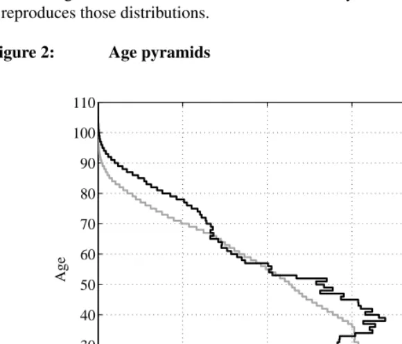
Let us consider the share of population at each age in total US population in 1950 and 2000. Using data obtained from the Human Mortality Database (HMD hereafter), Figure 2 reproduces those distributions.
Figure 2: Age pyramids
0 0.5 1 1.5 2 2.5
0 10 20 30 40 50 60 70 80 90 100 110
% of Total Population
Age
1950 2000
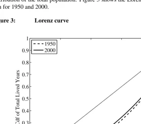
of a given age within the distribution of ages may have also changed. Otherwise stated, being 60 in 2000 may be totally different from being 60 in 1950. An extra normalization is needed. We believe that the examination of the Lorenz curve, depicting the cumulative distribution of the total years lived by a population at a given date against the cumulative distribution of the total population. Figure 3 shows the Lorenz curves of the US popula-tion for 1950 and 2000.
Figure 3: Lorenz curve
0 0.2 0.4 0.6 0.8 1
0 0.1 0.2 0.3 0.4 0.5 0.6 0.7 0.8 0.9 1
Cdf of Total Population
Cdf of Total Lived Years
1950 2000
Strikingly, there is not much discrepancy between two Lorenz curves, although the 2000 distribution is closer to the uniform distribution, which would be characteristic of a stationary population composed of individuals with rectangular survival curve. This reshaping of the age pyramid clearly appeared in Figure 2 and can be quantified by the computation of the Gini coefficient. It was 0.42 in 1950, it went down to 0.36 in 2000.
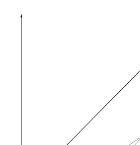
find three cutoff ages, denotedx1, x2andx3. Figure 4 reports a possible representation of the Lorenz curve derived from this new distribution together with the initial Lorenz curve.
Figure 4: Lorenz curves of the initial and modified distributions
6
-x1 x2 x3
Modified
Initial
N
Figure 5: Optimal grouping
0
0.5
1
1.5
2
2.5
0
50
100
1950
% of Total Population
Age
0
0.5
1
1.5
2
2.5
0
50
100
2000
% of Total Population
Age
3.2 Methodology
The problem of defining age groups amounts to approximating the age distribution of pop-ulation by a histogram that comprises a restricted number of age classes, that all gather individuals of different ages within a uniform group. There are two issues with such a process. The first one is to choose a number of classes. We adopt, as explained in the next section, a pragmatic approach to tackle this problem. A second issue regards setting the boundaries of each class. There is general agreement that there does not exist a unique definition of an age class. In particular, the boundaries of each group ought to be subjec-tive. As described previously, several criteria can be used to assess alternative definitions of age classes. Our approach is to define a grouping of single age-classes that preserves the characteristics of the age distribution. In other words, age groups are defined in such a way that they minimize the loss of information that occurs when building a histogram of the age pyramid using a given number of age classes. Aghevli and Mehran (1981) have developed a grouping technique that precisely addresses this issue, and applied it to income distributions.
We now describe how to apply Aghevli and Mehran’s method to age distribution. The optimal grouping aims at defining age groups that minimize the average difference of age pairs within each group, where the dispersion is measured with a Gini coefficient3. We
3Gini coefficients are a scale-independent measures of dispersion that has been applied to mortality
first present the case where a continuous distribution is discretized. Let us denote byf(·) the density of an age distribution on support[0, ω], such thatRω
0 f(x) dx= 1. Also letα denote the mean age of the population, such asα= R0ωxf(x) dx. The Gini’s absolute pairwise differences off(·), denotedG(f), writes:
G(f) = 1
α Z ω
0
Z ω
0
|x−z|f(x)f(z) dxdz.
For any integer n ≥ 2, we are looking for an n-cutoff representation of f(·). This amounts to defining a finite collection ofn+1real numbers, denotedx={x0, x1, ..., xn} and such that0 =x0< . . . < xn =ω, which induces a partition of the support off(·) intonnon-overlapping intervals. For alli = 1, . . . , n, let us define the integral of the density and the mean age for all intervals[xi−1, xi]:
yi=
Z xi
xi−1
f(x) dx, andαi=
Z xi
xi−1
xf(x) dx.
The Gini coefficient associated with a givenn−cutoff representation of f(·), denoted
G(f,x), write:
G(f,x) = 1
2α X i X j αi yi −αj
yj
yiyj.
Aghevli and Mehran (1981) suggest that one choose the collectionxthat minimizes the approximation errorε(f,x)as defined by the difference between the two Gini coeffi-cients:
ε(f,x)≡G(f)−G(f,x).
This approximation error can be rewritten as follows:
ε(f,x) = 1
2α
n
X
i=1
Z xi
xi−1
Z xi
xi−1
|s−z|f(s)f(z) dsdz.
Aghevli and Mehran show that the optimal collection of cutoff ages, denotedx? =
0, x?
1, ..., x?n−1, ω , satisfies:
x?i =
Rx?i+1 x?
i−1 xf(x) dx
Rx?i+1 x?
i−1 f(x) dx
,
In order to comment upon the optimal collectionx?, let us consider two simple ex-amples. First, in the particular case of two groups (i.e. forn= 2), it can be immediately deduced that the optimal cutoff age,x?
1, is the mean age of the population. Second, let us assume a uniform distribution such asf(x) = 1/ωfor allx∈[0, ω). The cutoff ages are computed by solving a system ofn−1equations that write:x?
i+1−2x?i +x?i−1= 0for alli= 1, ..., n−1, withx?
0= 0andx?n =ω. The solution is writtenx?i =iω/nfor alli. The above method, therefore, transforms a continuous into a discrete distribution. Population data are nevertheless provided through discrete age distributions, with one-year or five-one-year age groups in most cases. Our method hence consists in reducing the number of groups. Let us consider that the initial data provide ω groups indexed by
j = 0,1, ..., ω−1, that the frequency of group j in the total population is given by the quantitypj such thatP
ω−1
j=0pj = 1, and thatxj represents the mean age in group
j. We are looking for an optimal partition inton groups, with2 ≤ n ≤ ω, indexed byi = 0,1, .., n−1 or, equivalently for an optimal collection of cutoff ages, denoted
x? =
0, x?
1, ..., x?n−1, ω . The latter satisfies, for alli = 1, ..., n−1, the following system of equations:
x?i =
Pj
+
i+1−1
j=ji−−1xjpj+ j −
i−1−x?i−1
pj−
i−1−1xj
−
i−1−1+ x ? i+1−j
+ i+1
pj+
i+1xj +
i+1
Pj
+
i+1−1 j=ji−−1pj+ j
−
i−1−x?i−1
pj−
i−1−1+ x ? i+1−j
+ i+1
pj+
i+1
,
where ji−−1 = minj≥x? i−1
j−x?
i−1 is closest integer that is greater than x?i−1 and wherej+i+1= maxj≤x?
i+1
j−x?i+1 is the integer that is immediately lower thanx?i+1. The introduction of variables j− and j+ is necessary because optimal cutoff ages are unlikely to be integers.
Let us illustrate this latter case with the same examples as above. The simplest case is given for n = 2, where the optimal collection isx? = {0, x?1, ω}. We deduce that
j0− = 0and thatj2+=ωand thus:x? 1 =
Pω−1
j=0xjpj/P ω−1
j=0 pj. The case of a uniform distribution, which can also be studied analytically, is presented in Appendix 6..
Once we obtain the optimal partition of the distribution, it is possible to define simple aging indicators. In particular, we will consider two standard indicators. The first reports the share of the oldest group in the total population. It correspond to the share of people between agesx?
n−1andω,wherex?n−1has been defined above. More precisely, the share is written:
Z ω
x? n−1
f(x) dx.
the share of oldest group over the share of the youngest group:
Rω
x? n−1
f(x) dx
Rx?1
0 f(x) dx
.
Our indicators have the nice property of being invariant to any proportional rescaling of the age distribution accompanying an increase in life expectancy. The formal proof of this property is proposed in Appendix 6..
4.
The dynamics of population aging in industrialized countries
In this section, we evaluate the dynamics of aging in industrialized countries using HMD data for the age structure of population. We first present the case of the US population and then proceed to an international comparison.
4.1 Aging in the US
Our data document the size of the US population at each age between birth and age 110 for the year 1933 through 2005. We choose to divide the population age distribution into 4 groups. This choice is made for pragmatic reasons and comparative purposes. It indeed leads to cutoff ages for the youngest and oldest groups of about 15 and 60 in the end of the 1990s in the international comparison we will carry out below. We will, however, assess the robustness of our results regarding number of groups in the next subsection.
Figure 6 reports the evolution of the entry age into the oldest group (left panel) and the share of that group (right panel) within total US population.4
A first result that emerges from the left panel is that the entry age in the oldest group has increased over time. For instance, in 1933 the cutoff age was 48.7, while it rose to 56.6 in 2005 -a 16.22% increase. In order to make sense of this result, let us consider an individual of age 55. In 1933, this individual would have been classified as belonging to the group of the oldest. This is no longer the case in the current US society. Otherwise stated, at age 55, a US individual is younger in 2005 than in 1933. At first glance, this phenomenon can be attributed to individual aging, as captured, for example, by life ex-pectancy. For instance, life expectancy at age 55 was 19.2 years in 1933. It was 26.7 years in 2005. This idea of a time varying old age is already present in Ryder (1975) and subse-quent literature. However, as mentioned above, the optimal grouping approach makes use of the entire distribution, which implies that this increase in the cutoff age does not solely reflect changes at the individual level, but any change in the shape of the distribution.
Figure 6: Share of elderlies
1940 1960 1980 2000 48
50 52 54 56 58
Years
Age in Years
3rd Cutoff Age
1940 1960 1980 2000 0.18
0.19 0.2 0.21 0.22
Years
Share of the Oldest Individuals
Once we allow for the time-varying cutoff age, the share of the oldest group in total US population can be computed. This share can be seen as an alternative measure of aging that corrects for a time-varying entry age into the oldest group. Its evolution is reported in the right panel of Figure 6. It appears that the share of the oldest group has exhibited variations over time around an average value of 20.48%. These movements are quite sig-nificant, as reflected by a standard deviation of about 0.5 points. More importantly, there is no trend in the evolution of this ratio over the considered time window.5 According to this indicator, the US has not aged. In other words, the US simply experienced an upward translation in the age pyramid for the oldest ages over the time window that has been compensated for an increase in the age when an individual becomes old.
It is, however, important to note that most of the changes in the US age pyramid took place in the young ages (as it can be seen in Figure 2). The significant narrowing in the bottom of the pyramid suggests that the ratio of old to young individuals ought to have increased markedly over the last 50 years. This fact is usually interpreted as aging. We now investigate this issue. Figure 7 reports the evolution of the age at which an individual exits the group of the youngest (left panel), and the share of that group in total US population (right panel).
Over the entire time window, the cutoff age has increased by 27% (15 in 1933, 19 in 2005). This increase can also be attributed to the evolution of life expectancy: in a society where life is longer on average, so is youth. However, it displays swings in its evolution, which can be related to the post WWII baby-boom. With our measure, the
first and direct effect of a baby-boom is to reduce the average age of the youngest group. Consequently, the oldest former members of this group will be excluded and reassigned to the next group. Hence, the cutoff age will decrease. This is exactly what we observe until the early sixties. As baby boomers grow older, there is an upward pressure on the average age of the youngest group and the direct effect of the increase in the life expectancy comes into play. When baby boomers start to have children, there is an echo effect that dampens the increase in the cutoff age. This can be seen in the deceleration in the evolution of that age which took place in the late seventies. This evolution translated to that of the share of the youngest group in total US population. Just like the evolution of the share of the oldest group, the share of young individuals does not display any significant trend. It however exhibits large fluctuations around its mean (27.6%) with a standard deviation of 1.22 points. The share of the young population increased during the baby-boom, despite the diminishing cutoff age.
Figure 7: Share of the young
1940 1960 1980 2000 13
14 15 16 17 18 19
Years
Age in Years
1st Cutoff Age
1940 1960 1980 2000 0.23
0.24 0.25 0.26 0.27 0.28 0.29
Years
Share of the Youngest Individuals
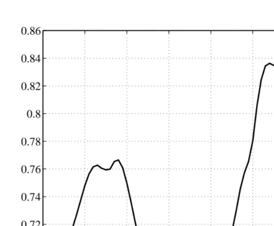
We are now in a position to compute the elder-child ratio, which, in our case, is com-puted as the ratio of the size of the group of the oldest to that of the youngest individuals. This ratio is shown in Figure 8.
Figure 8: Elder-child ratio
1930 1940 1950 1960 1970 1980 1990 2000 0.68
0.7 0.72 0.74 0.76 0.78 0.8 0.82 0.84 0.86
Years
4.2 On the number of groups
We now assess the robustness of our results againt change in number of groups. We consider four alternative values for the number of groups,n, ranging from three to six.6 Figure 9 reports the evolution of the share of the oldest group (top-right panel), the share of the youngest group (top-left panel) and the elder-child ratio (lower panel).
As should be expected, the level of the shares crucially depends on the number of groups: the larger the number of groups, the lower the share. However, the overall evo-lution of the shares is quite similar. In particular, the evoevo-lution of the share of the oldest group indicates that, no matter the number of groups, aging is very limited. The elder-child ratio should provide us with a way to assess the robustness of our approach, as it should be level invariant. As seen from the lower panel of Figure 9, the elder-child ratio lies within the same range of values for all values ofn. It is nevertheless true that the
namics are not exactly the same, and, most notably, the ratio computed in the four groups models features an opposite trend in the 1960’s and the early 2000’s. Nevertheless, as reported in Table 1, the ratios, as computed with different numbers of groups, are highly positively correlated.
Figure 9: Robustness to the number of groups
1940 1960 1980 2000 0.2
0.25 0.3 0.35 0.4
Years
Share of Youngest Individuals
1940 1960 1980 2000 0.1
0.15 0.2 0.25 0.3 0.35
Years Share of Oldest Individuals
1930 1940 1950 1960 1970 1980 1990 2000
0.65 0.7 0.75 0.8 0.85
Years Elder−Child Ratio
n=3 n=4 n=5 n=6
Table 1: Correlation of elder–child ratios
n 3 4 5 6
3 1.00 0.71 0.75 0.73 4 – 1.00 0.77 0.74 5 – – 1.00 0.89
This indicates that the properties of the aging indicator, as derived from optimal group-ing, is robust to choice of the number of groups when the time window is sufficiently long. However, for short run assessments, the number of groups may be an issue.
4.3 An international perspective
The previous section has shown for the US economy that aging may not be as pronounced when we take into account that the age of entry into old age varies over time. We now investigate whether this result extends to other industrialized economies. We use an-nual data from the HMD for Australia, Austria, Canada, Denmark, France, Iceland, Italy, Netherlands, Norway, Spain, Sweden, Switzerland, England & Wales. The time period covered by the HMD runs from 1751 (for Sweden only) to 2005. However, for compar-ison purposes and for data quality reasons, we are going to focus on the last 50 years of the time window, i.e. from 1955 to 2005. As in the case of the US, we choose to split the population into four groups, for practical reasons.
For each country and each year, we computed the cutoff ages for old and young and, on the left panel, the shares of the old and young groups in total population, and the share of old to that of young individuals.
According to our computations, international aging, as measured by the share of old people in total population, is mitigated. The share exhibits fluctuations in all the countries, with standard deviations ranging from a low 0.49 points in the US to a high 1.63 points in England & Wales. However, the share appears to be remarkably stable over time and remains close to 20% in most countries of our sample. Patterns for the age below which an individual is classified as young are very similar to those obtained in the US case. The cutoff age increased in all countries. At low frequencies, this can be related to the increase in life expectancy at birth. In particular, we observe the same acceleration in the cutoff age as the one we observed in the threshold determining old age. Interestingly, we recover the same effects of baby–booms in all countries that experienced them. In all these countries, the cutoff age decreased in the mid–sixties.
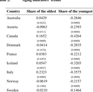
In order to investigate this issue more precisely, we compute the average annual rate of growth of the share by fitting a linear trend to the logarithm of the share. This is done for the last 50 years in each country and the results are presented in Table 2.
ex-perienced negative growth in this share over the last 50 years, suggesting a rejuvenation of their populations.
Table 2: Aging indicators’ trends
Country Share of the oldest Share of the youngest Elder-child ratio
Australia 0.0429 -0.2846 0.3275
[0.0422] [0.0000] [0.0000]
Austria -0.0963 -0.2393 0.1430
[0.0311] [0.0000] [0.0452]
Canada 0.1652 -0.4264 0.5916
[0.0000] [0.0000] [0.0000]
Denmark -0.0414 -0.2835 0.2421
[0.1676] [0.0000] [0.0000]
France 0.0383 -0.2212 0.2595
[0.4493] [0.0000] [0.0010]
Iceland 0.0547 -0.3203 0.3750
[0.0057] [0.0000] [0.0000]
Italy 0.2323 -0.3575 0.5898
[0.0000] [0.0000] [0.0000]
Norway -0.0619 -0.2157 0.1538
[0.1486] [0.0000] [0.0266]
Sweden -0.0210 -0.1464 0.1254
[0.6051] [0.0002] [0.0867]
Switzerland -0.0440 -0.2335 0.1895
[0.0404] [0.0000] [0.0001]
UK -0.0010 -0.1428 0.1418
[0.9756] [0.0001] [0.0158]
USA -0.0173 -0.2937 0.2764
[0.4646] [0.0000] [0.0000]
Notes: Growth rate in % of a given indicator as obtained from an OLS regression of the log of the indicator on a constant term and a linear trend. p-value of nullity test is in brackets.
in Iceland and 1.74 points in England & Wales. In particular, these fluctuations echo the evolution of the cutoff age during the baby–boom.
Concerning the ratio of the share of old to that of young individuals, Table 2 indicates that most countries display a significant and positive trend. It is however worth noting that the growth rates are all below 0.6%. Moreover, as in the US case, this ratio displays much variability. In particular, baby-booms all yield a rejuvenation of the population in their later phase. Likewise, in continental Europe, wars lead to a rejuvenation in their aftermaths as many middle–aged people are killed and the fertility rate drops. Therefore after wars, there are more people with high age, and consequently the age below which an individual is classified as young increases which leads to a decrease in the corresponding share. Henceforth the elder–child ratio increases.
5.
Conclusion
This paper proposes an alternative measure of aging that resorts to optimal grouping tech-niques. This approach leads to an endogenous definition of old age that depends on the entire distribution of ages within the population. Therefore the old age cutoff ought to depend on the type of population, the country and the date at which it is evaluated. For instance, in the US this age at which one is considered a senior has increased dramati-cally over last century. Despite the potential high sensitivity of this old age cutoff to the distribution, most industrialized countries exhibit a very similar pattern. Likewise, we find that, contrary to the common arguments for an aging population, the share of elderly individuals within the total population has not increased much and has remained stable in these countries. Likewise, we find that, contrary to the common arguments of an aging population, the share of elderly individuals within the total population has not increased much and has remained stable in these countries. These results complement and rein-force the earlier findings of Sanderson and Scherbov (2005, 2007) who also reassessed the aging phenomenon.
The main advantage of the measure we propose is to offer a new method for calculat-ing the cutoff ages of major age groups such as adulthood and old age. The weight we assigned to each age is proportional to its frequency in the age distribution but one may consider other weights including economic, health or productivity considerations. Hence, our approach could be applied to the study of medical spendings as in Cutler and Sheiner (2001), dependency ratios as in Oliveira Martins et al. (2005) and the labor force as in Shoven (2010). It could also be used to evaluate the importance of forecasted population trends in terms of aging and be extended to incorporate disability status as in Sanderson and Scherbov (2005, 2007).
the share of elderly in a given population, depends on the initial choice of the number of groups. We have shown that over a sufficiently long interval of time, our measure was not sensitive to choice of number of groups. However, in the short run, this choice may have an impact. An interesting extension of our work would be to use the recent work of Poggi (2005) who proposed a method to optimally determine a number of groups.
6.
Acknowledgements
References
Aghevli, B.B. and Mehran, F. (1981). Optimal grouping of income distribution data. Journal of the American Statistical Association76(373): 22–26.doi:10.2307/2287035.
Bourdelais, P. (1994). L’Age de la Vieillesse. Histoire du Vieillissement de la Population. Paris: Editions Odile Jacob.
Bourdelais, P. (1999). Demographic aging: A notion to revisit.The History of the Family: An International Quarterly4(1): 31–50.doi:10.1016/S1081-602X(99)80264-4.
Chu, C.Y. (1997). Age-distribution dynamics and aging indexes. Demography34(4): 551–563.doi:10.2307/3038309.
Coulson, M.R.C. (1968). The distribution of population age structures in kansas city. An-nals of the Association of American Geographers58(1): 155–176. doi:10.1111/j.1467-8306.1968.tb01641.x.
Cutler, D.M. and Sheiner, L. (2001). Demographics and medical care spending: Standard and non standard effects. In: Auerbach, A. and Lee, R. (eds.).Demographic Change and Fiscal Policy. Cambridge: Cambridge University Press: 253–291.
Davies, J.B. and Shorrocks, A.F. (1989). Optimal grouping of income and wealth data. Journal of Econometrics42(1): 97–108.doi:10.1016/0304-4076(89)90078-X.
Esteban, J., Gradín, C., and Ray, D. (2007). An extension of a measure of polarization with an application to the income distribution of five oecd countries. Journal of Eco-nomic Inequalities5(1): 1–19.doi:10.1007/s10888-006-9032-x.
Fenge, R., de Ménil, G., and Pestieau, P. (2008). Pension Strategies in Europe and the United States. CESifo Seminar Series. Cambridge MA: The MIT Press.
Foster, J.E. and Shorrocks, A.F. (1988). Poverty orderings. Econometrica56(1): 173– 177. doi:10.2307/1911846.
Goldstein, J.R. and Wachter, K.W. (2006). Relationships between period and co-hort life expectancy: Gaps and lags. Population Studies 60(3): 257–269.
doi:10.1080/00324720600895876.
Human Mortality Database (2013). Human mortality database. [electronic resource]. University of California, Berkeley (USA) and Max Planck Institute for Demographic Research (Germany).www.mortality.org.
Le Grand, J. (1987). Inequality in health: Some international comparisons. European Economic Review31: 182–192.
Lee, R. and Goldstein, J.R. (2003). Rescaling the life cycle: Longevity and proportional-ity.Population and Development Review29: 183–207.
Nath, D. and Islam, M. (2009). New indices: An application of measuring the aging process of some asian countries with special reference to bangladesh.Journal of Pop-ulation Ageing2(1–2): 23–39.doi:10.1007/s12062-009-9016-2.
Oliveira Martins, J., Gonand, F., Antolín, P., de la Maisonneuve, C., and Yoo, K.Y. (2005). The impact of ageing on demand, factor markets and growth. OECD Economics De-partment. (Working Paper 420).
Poggi, A. (2005). Endogenous population subgroups: The best population partition and optimal number of groups. Departament d’Economia Aplicada. Universitat Autònoma de Barcelona. (Document de Treball 05.08).
Ryder, N.B. (1975). Notes on stationary populations. Population Index41(1): 3–28.
doi:10.2307/2734140.
Sanderson, W.C. and Scherbov, S. (2005). Average remaining lifetimes can increase as human population age.Nature435(7043): 811–813. doi:10.1038/nature03593.
Sanderson, W.C. and Scherbov, S. (2007). A new perspective on population aging. De-mographic Research16(2): 27–58. doi:10.4054/DemRes.2007.16.2.
Sanderson, W.C. and Scherbov, S. (2010). Remeasuring aging.Science329(5997): 1287– 1288.doi:10.1126/science.1193647.
Shkolnikov, V.M., Andreev, E.E., and Begun, A.Z. (2003). Gini coefficient as a life table function: Computation from discrete data, decomposition of differences and empirical examples.Demographic Research8(11): 305–358. doi:10.4054/DemRes.2003.8.11.
Shoven, J.B. (2010). New age thinking: Alternative ways of measuring age, their rela-tionship to labor force participation, government policies and gdp. In: Wise, D.A. (ed.). Research Findings in the Economics of Aging. National Bureau of Economic Research: 17–31.
Appendix
A toy-example of optimal grouping
Let us present an analytical example of optimal grouping applied to a discrete age distri-bution, which is assumed to be uniform. This case is obtained by assumingpj = 1/ωfor allj, and thus, the optimal collection of cutoff ages satisfies:
x?i x?i+1−x?i−1
=
ji++1−1
X
j=ji−−1
xj+ ji−−1−x ? i−1
xj−
i−1−1
+ x?i+1−ji++1
xj+
i+1
,
for alli = 1, ..., n−1. One has also to define the mean age in a given group. Let us suppose thatxj = j + 0.5 for allj = 0,1, ..., ω−1. The previous equation can be rewritten as follows:
(x?i −0.5) x?i+1−x?i−1
= j
− i−1 j
− i−1−1
−ji++1 ji++1+ 1
2
−x?i−1 ji−−1−1
+x?i+1ji++1.
As a numerical application, let us suppose that there are initially 10 groups and that one wants a representation into 3 groups. Hence, one hasω = 10, n = 3, j0− = 0and
j3+= 10and the problem is to find x? 1, x?2, j
−
1, j + 2 that solves:
(x?
1−0.5)x?2=−
j2+(j+2+1) 2 +x
? 2j
+ 2
(x?
2−0.5) (10−x?1) =
j1−(j1−−1) 2 −x
? 1 j
−
1 −1
+ 45
j−1 = minj≥x?
1{j−x ? 1}
j+2 = maxj≤x?
2{j−x ? 2}
Proof of invariance to proportional rescaling
As defined by Lee and Goldstein (2003), proportional rescaling would appear indistin-guishable from the effect of a simple change in the units of measurement of age/time. A population whose age distribution has been proportionally rescaled should of course not be considered as older.
Consider the density of age distributionf(·)on support[0, ω]with cumulative distri-bution functionF(a) =Ra
0 f(x) dx. A distributionh(·)on support[0, ω
0]whereω0> ω
is a proportional rescaling off if:
H
aω
0
ω
=F(a), ∀a∈[0, ω],
whereHis the cumulative distribution function ofh(·).
Using an aging index with a fixed cutoff denoteda0 would misleadingly indicate a aging of the population asH(a0) < F(a0)for alla0 ∈ [0, ω]. Using Ryder’s (1975) index would also yield an unpleasant result. Letaf andah be respectively the age at which an individual has a given life expectancy, e. g. 10 years, in distribution f(·) andh(·)respectively. af andah define the cutoff ages of entry into old age, and since generically,afω 6=ahω0, the Ryder index would assimilate the proportional rescaling as either a population aging or a rejuvenation.
Let us now turn to our indicators built using the optimal cutoffs defined as follows:
xi,f =
Rxi+1,f
xi−1,f xf(x) dx
Rxi+1,f
xi−1,f f(x) dx
andxi,h=
Rxi+1,h
xi−1,h xh(x) dx
Rxi+1,h
xi−1,h h(x) dx
,
where the?’s are eliminated to simplify notation. After some simple algebra, we obtain:
ω ω0xi,h=
Rωω0xi+1,h ω ω0xi−1,h
xf(x) dx
Rωω0xi+1,h ω ω0xi−1,h
f(x) dx ,
which implies thatxi,h =xi,fω0/ω. Consequently, the share of the oldest group in the total population is left unaffected by a proportional rescaling:
Z ω
xn−1,f
f(x) dx=
Z ω0
xn−1,h