0 INTRODUCTION
Nowadays most production processes are designed to increase economic efficiency while, at the same time, not influencing product quality, especially when dealing with large serial production. In order to improve the forming process from the economic point of view, the main objective is to minimize the number of operation phases involved in the forming process. The cutting phase, as the final operation, is the phase most often targeted for elimination. Along with less material required for product production, the elimination of the cutting phase may also reduce the occurrence of manufacturing defects during the forming process, such as tearing and wrinkling. In some cases, however, the sheet cutting phase is unavoidable since excess material under the blank-holder is required to achieve proper holding of the sheet metal [1].
When the cutting phase is eliminated, the accuracy of the product edge geometry should be provided by proper blank shape geometry. In most cases, the proper blank shape is determined experimentally by a trial and error procedure which requires several try-outs, causing the forming process design to be extremely time consuming and costly. Nowadays, this can be done virtually, based on computer simulations of the technological process under consideration, see, for example, [1] to [4]. Besides choosing a proper numerical approach and computational technique [5] and [6], advanced constitutive modelling [2], [4], [7] and [8] and proper material characterisation [4] and [7] to [9] is crucial for the computer simulation
to be physically objective and trustful. Although, in contrast to direct analysis, a Finite Element (FE) inverse analysis approach, see [10] to [14], could possibly be used in sheet metal forming simulation in order to reduce the computer time consumption, such an approach is not recommended because it results in less accurate strain–stress state determination. This, in turn, can considerably influence the subsequent springback analysis, which is a key element in tool design optimisation.
This paper describes a blank shape optimisation method, which allows determination of a blank shape such that the edge geometry deviation of the produced product with respect to the specified product geometry is obtained within a given tolerance. In this method, the optimal blank shape is determined in an iterative way, starting with an initial blank of approximately adequate shape, which over a series of subsequent iterations gets automatically adjusted to meet the tolerance criterion. Following the principal idea, which is a gradual changing of the given blank shape based on the computed product geometry and manifested edge deviation, the product geometry must be determined in each iteration by a corresponding forming process simulation, considering the blank shape as determined in the previous iteration.
The method is designed in such a way that it enables optimal blank shape determination of products having a general 3D shape. That the method is capable of tackling rather complex product geometries efficiently is demonstrated in Section 4, where results of the numerical optimisation process are also experimentally validated.
A Method for Optimal Blank Shape Determination in Sheet Metal
Forming Based on Numerical Simulations
Mole, N. – Cafuta, G. – Štok, B.
Nikolaj Mole1 – Gašper Cafuta2 – Boris Štok1,*
1 University of Ljubljana, Faculty of Mechanical Engineering, Slovenia 2 Cimos d.d., Automotive industry, Slovenia
The main benefit of using optimally shaped blanks in sheet metal forming is to maximize the efficiency of the forming process and, since there is no need for additional cutting operations after the finished forming operation, this leads to a substantial reduction in overall production costs. This paper presents a numerical method for optimal blank shape determination, which is suitable in various sheet metal forming applications. The optimal blank shape is determined in an iterative way so that the edge geometry of the formed product fits its reference geometry as closely as possible. The iterative process starts with the blank shape from which the product is produced with its edge fitting its reference geometry just approximately. In subsequent iterations, the blank shape is continuously improved in accordance with the developed optimisation method. In order to determine the product edge geometry resulting from the given blank shape, a computer simulation of the forming process and related springback is performed at each iteration. Since its effectiveness greatly depends on the quality and physical objectivity of the computer simulation, the developed numerical blank shape optimisation procedure has also been validated experimentally by using the forming of a product with a rather complex edge geometry as the case study.
1 REVIEW OF SOME APPROACHES TO BLANK SHAPE OPTIMISATION
The problem of finding an appropriate blank shape, which would allow the production of a formed product with the edge geometry meeting the geometry tolerance requirements, as specified by the design, has been addressed by many authors. In the section, we give a brief review of different numerical approaches developed in this regard.
An optimisation method, where the initial blank shape approximation is determined by inverse FEM simulation and the blank shape is optimised iteratively afterwards using direct FEM computer simulations, is presented in [15] and [16] by Azaouzi et al. The applied blank shape modification consists of displacing, in each iteration, the blank edge nodes in the direction opposite to the geometry deviation obtained by comparing the computed and reference product geometry. After the new blank shape is determined, its domain is remeshed automatically using triangular FEs. Naceur et al. [17] presented a blank shape optimisation approach that is based on the coupling between the inverse approach used for the forming simulation and an evolutionary algorithm. Their goal was to minimize the size of the blank shape and still ensure that the product is made without tearing the sheet metal. Park et al. [18] introduced a deformation path method. The Ideal Forming direct inverse design method, see [13] and [14], was used to determine initial blank shape, which was further improved by an iterative procedure. In [19], Yeh et al. use the inverse true strain method (TSM) to obtain an initial approximation of the blank shape, whereas for the optimal blank shape determination a method based on adaptive-network-based fuzzy inference system (ANFIS) is applied. To achieve satisfactory results on the optimised initial blank shape, at least for the case considered in the paper, 200 learning cycles, each requiring a complete computer simulation of the corresponding forming process, had to be used in building the appropriate ANFIS database. Another approach, where the abductive network is used to predict the optimal blank shape for forming an elliptic cup using FEM computer simulations, is presented by Lin and Kwan in [20]. In the optimisation procedure, the initially elliptic blank shape, with its geometry being specified in a polar coordinate system by four characteristic points, is subject to change by considering adequate variation of the respective points’ radial coordinates, while keeping their angular coordinates fixed. An iterative method, where the product geometry is also computed using inverse
FEM while the blank shape correction is made in each iteration manually, is introduced by Parsa and Pournia in [21]. Due to the application of the inverse analysis approach, the computational time is significantly reduced, but it is achieved at the expense of loss of accuracy in the product geometry determination.
The objective of the blank shape optimisation presented in [22] by Pegada et al. is to determine the blank shape that allows forming of a circular cup of uniform height, where the respective material properties are assumed to be orthotropic. In each iteration, considering the established deviation in the cup height, the blank shape is adapted proportionally, assuming a value of 0.75 as an adequate scaling factor to obtain satisfactory convergence to the method. In the method introduced by Son and Shim in [23], the blank shape correction is made in the direction opposite to the geometry deviation obtained by comparing the computed and reference product geometry. Furthermore, correction of each edge point is computed by applying a scaling factor between 0.5 and 0.9, its actual value being defined by a ratio of the initial velocity to the total deformation path length. In [24], Hamammi et al. propose a method where the blank shape correction is made in the direction described by the positions of each node lying on the blank edge at the beginning and at the end of the forming process. Another method, where the correction of the blank shape is also based on taking the displacement path of the product edge nodes into account, is proposed by Fazli and Arezoo in [25]. They proved that their method is slightly better in terms of accuracy and also in convergence than the previous two methods, [23] and [24].
The optimal blank shape can also be obtained by parameterisation of the blank geometry and using a sequential programming method for finding the optimal set of parameters, which is elaborated in [26] by Sattari et al. Similarly, in [27], Padmanabhana et al. investigate blank shape optimisation using parameterisation of the blank shape carried out by using parametric NURBS curves and the blank shape correction based on the control points displacement. The convergence of the latter method can be further improved by including the sensitivity analysis shown in [28] by Shim et al.
The iterative approach we present here is implemented in such a way that the user must provide an approximately determined blank shape, which is taken as the initial blank shape for the optimisation procedure. As demonstrated by the study case, elaborated in Section 4, the proposed numerical approach is efficient enough that it does not require a very accurate determination of the initial blank shape, which is the case in [15], [16], [18] and [19]. By using different strategies the user can still provide a better approximation for the initial blank shape, which is certainly advantageous. One thing that is common to all the methods presented in the review is that, in each iteration, a remeshing of the blank is required after blank shape correction. In our case, on the other hand, the mesh element topology is kept unchanged through the entire iterative procedure, while the corresponding FE mesh nodal points’ adjustment in the iteration is performed in accordance with the displacement field obtained by solving an associate linear elastic boundary value problem. In this boundary value problem, the blank with the actual shape geometry before correction is subjected to prescribed boundary displacements, the imposed boundary displacements taken equal the required blank edge geometry correction in the iteration. With the blank FE mesh correction dealt with in this way, any type of FEs can be used and no sophisticated remeshing methods are needed.
2 MATHEMATICAL, MODELLING AND PHYSICAL PRELIMINARIES
In order to provide a corresponding mathematical framework for the numerical analysis, in this section we give some definitions and conventions on the geometry terminology used, which is followed by a determination of some related point topology quantities, such as surface and edge normal vectors’ determination, and, finally, an approximation for analytical surface reconstruction.
Some modelling and simulation assumptions are given in the last part of the section in order to focus our investigation on the key elements of the proposed numerical procedure for the blank shape optimisation described in Section 3.
2.1 Geometry and Point Topology Terminology
In this paper, we adopt the same geometry terminology as introduced by Cafuta et al. in [29]. The product geometry prescribed by the design engineer is referred as the “reference geometry”, whereas the
product geometry computed in the simulation will be referred as the “actual geometry”. Considering that the forming process simulations are performed on the basis of FEM, we are actually dealing with discretised
geometries. In accordance with the notation G,
introduced for a general surface point topology
definition, we will use notations Gref and Gact to
specify point topologies related to the reference and actual product geometry, respectively. Similarly,
notation Gbl will be used to denote point topology
related to the sheet blank geometry. Furthermore,
Γref, Γact and Γbl will be used to specify the
associated edge point topologies notations. All those surface and edge topologies will exclusively refer to the sheet’s mid-surface. In addition, to support a numerical procedure of automatic sheet blank geometry adjustment, an auxiliary virtual surface
with its point topology notation being Σ
G will be
generated, emanating from the reference product edge
Γref considering its surface topological properties.
The surface Σ
G having properties Γref ⊂ Σ
G may be
considered as a target surface which is to be attained
iteratively by the edge points ΓP
ik of the actual
product Γactk as closely as possible.
Since, in the numerical procedure, the unit normal
vectors ni at point Pi perpendicular either to the
surface or to the edge will also be referenced, it is reasonable to make a symbolic distinction between
them. Accordingly, the notations ni and Σni will be
used for the surface normal vectors, whereas
Γn
i will be used for the edge normal vectors.
Similarly, to make a distinction between the points
appertaining either to the product surfaces, Gref and
Gact, or to the auxiliary surface ΣG , the notations Pi
and ΣP
i will be used with respective position vectors
being Pi and ΣP
i. If point Pi is located on the edge Γ,
it will be denoted as ΓP
i and its position specified by
vector ΓP
i.
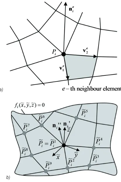
2.2 Surface Normal Vector Determination
The accuracy of the surface normal vector determination at points of discretely given surface geometries plays an important, if not crucial, role in attaining convergence and speeding up the convergence rate of the entire optimisation procedure.
A general surface point topology G given, we apply
in this paper a two-step procedure in which for a point of interest, say Pi, two auxiliary vectors, n′i and n′′i , are computed, respectively.
The following equation is used:
′ ×
×
∑
∑
n n
n
n v v
v v
i e
Ni i e
e Ni
i e
i
e e e
e e
= =1 , =
=1
1 2 1 2
, (1)
with Ni being the number of neighbouring FEs
connected to point Pi and nie being their respective
normal vectors at that point. The latter are determined
by considering the respective FE’s edge vectors v1e
and v2e emanating from point Pi (Fig. 1a).
a)
b)
Fig. 1. Surface normal vector determination: a) FE’s nodal normal vector nie determination, and b) auxiliary vector n′′i determination
In the second step, the normal vector ni is
determined considering the analytically defined
smooth surface Si through point Pi. This surface is
obtained by a corresponding interpolation through a point set Πi, built from points P jij( = 1,2,...,9) of the FE mesh. Those points are chosen from a sub-domain
area surrounding the considered point P Pi ≡ i1 on a
closest point’s basis, which is applicable regardless of
whether point P Pi ≡ i1 belongs to the interior of the FE
mesh or to its boundary.
Mathematical representation of the surface Si ,
F x y zi( , , ) = 0, is built by considering coordinates of
the respective points of the set Πi. To avoid round-off
error due to possible computing with large numbers, it
is advantageous to have the surface Si representation
defined with respect to a particular local coordinate system, say ( , , )x y z , having its origin at point P Pi≡ i1 (Fig. 1b). The base vectors e e ex, , , defining the y z respective local coordinate system ( , , )x y z at point
Pi in accordance with the above stated properties, are
determined by expressions:
ex=e n r ez× ′i = , y=e e ez× x, z=n′i , (2)
where the base vector ez = (0,0,1) defines the global
coordinate axis z.
The rotation of the global coordinate system (x, y, z) to the local coordinate system ( , , )x y z is given
by the rotational transformation matrix ℜ( , )rθ :
ℜ
( , ) =rθ ,
a b c c a b b c a
xx xy xz
yx yy yz
zx zy zz
(3)
where the matrix coefficients are determined as:
a r v b rr v r c rr v r
ii i
ij i j k
ij i j k
= +
= −
= +
2 ( ) cos( )
( ) sin( )
( ) sin(
θ θ
θ θ
θ θθ) ; i j k i≠ ≠ ≠ . (4)
Above, rx, ry and rz are the components of
vector r=( , , )r r rx y z and quantity v( )θ is defined
by v( ) = 1θ −cos( )θ , the angle θ denoting the angle
between the base vectors ez and ez.
To enable analytical surface Si representation
f x y zi( , , ) = 0 with respect to the local coordinate system ( , , )x y z , the coordinates of the position vector
Pij are mapped to the local coordinate system in
accordance with:
Pij r P P
ij i
= ( , )ℜ θ
(
−)
. (5)With the points set Π
i consisting of nine points
Pij (Fig. 1b), it is appropriate to approximate surface
Si in accordance with:
f x y zi z a x y
m n mn
m n
( , , ) = = 0 ,
=0 2
=0 2
−
∑∑
(6)where nine coefficients amn are determined such that
Finally, the auxiliary vector n′′i normal to the
surface f x y zi( , , ) = 0 at point Pi1(0,0,0) can be determined by the gradient operator:
′′
ni i
i
f f
= (0,0,0)
(0,0,0) .
grad
grad (7)
By applying to the components of the above vector, given in the local coordinate system, the
inverse mapping ℜ−1( , )rθ , the components of the
normal vector ni to the surface Si at point Pi in the
global coordinate system are obtained such that:
ni =ℜ−1( , )rθ ni′′. (8)
If the point, at which the normal vector is to be computed, is positioned on the symmetry plane, the
normal vector ni is computed by the same procedure
considering the mirror elements over the symmetry plane.
The abovedescribed procedure of the surface normal vectors’ determination is general. In Section 3, it will be carried out with reference to the reference
and actual product geometry, Gref and Gact, as well as
to the auxiliary surface ΣG .
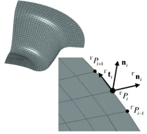
2.3 Edge Normal Vector Determination
We will refer generally to a surface point topology
G and associate edge point topology Γ also in the
determination of the unit vectors normal to the edge of a bounded surface. At a point of interest on the
boundary Γ, say ΓP
i, the edge normal vector Γni
will be determined considering respective surface and boundary curvatures. While the surface curvature is characterised by the respective surface normal vector
ni, with its determination being described in Section
2.2, the boundary curvature can be characterised by a
unit vector Γt
i tangential to the surface boundary at
point ΓP
i.
The tangential vector Γt
i can be correspondingly
approximated considering actual discretisation of the
boundary Γ in the closest vicinity of the point ΓP
i.
With points ΓP
i−1 and ΓPi+1 being the points adjacent
to point ΓP
i (see Fig. 2) the following equation may
be applied:
Γ Γ Γ
Γ Γ
t P P
P P
i i i
i i
= 1 1
1 1
+ −
+ −
−
− . (9)
Finally, by evaluating the vector product:
Γn Γt n
i = i× i, (10)
the edge normal vector Γn
i, defined in the global
coordinate system, can be determined. The corresponding graphical representation, with vector
Γn
i lying in the tangential plane to surface Si and
pointing to its exterior, is given in Fig. 2.
If the point, at which the edge normal vector is to be computed, is positioned on the symmetry plane, in order to achieve geometric symmetry conditions,
the tangential vector Γt
i is defined by a unit vector
normal to the symmetry plane. The edge normal vector
Γn
i is afterwards computed by the same procedure.
Fig. 2. Edge normal vector Γni determination
2.4 Analytical Surface Reconstruction
Assuming that the considered FE surface discretisations are all based on a quadrilateral surface element meshing (see Fig. 1), we will develop, in this section, an approximation to the analytical surface reconstruction of a single quadrilateral surface element, considering its particular topological properties.
Let a quadrilateral surface Si be discretely
defined by its nodal points P jij( = 1,2,3,4) and
respective surface normal vectors nij at those
points, determined following the procedure described in Section 2.2. This set of data represents twelve independent parameters, which can be used in
analytical surface reconstruction of surface Si ,
F x y zi( , , ) = 0. This can be achieved by considering the following functional form:
F x y z z a a x a y a x y a x a y a x y a
i i i i i
i i i i
( , , ) = ( 1 2 3 4
5 2 6 2 7 2 8
− + + + +
+ + + +
xxy
a x yi a x a yi i a x yi
2
9 2 2 10 3 11 3 12 3 3) = 0
+
+ + + +
, (11)
with twelve coefficients a mmi ( = 1,2,...,12) to be
interpolation points Pij the following system of linear equations is obtained:
F x y z F
x x y z n n F
y x y z
i j j j
i
j j j i x
j
i zj
i
j j j
( , , ) = 0
( , , ) =
( , , ) =
, ,
,
,
∂ ∂ ∂
∂
nn n j
i yj i zj
, ,
; = 1,2,3,4 , (12)
whose solution yields the value of the coefficients
ami . Here, it should be emphasised that by fulfilling
the nodal surface properties in the above way element
after element C1 continuity at discrete points of the
surface Si is achieved, which is significant for the
quality of the overall surface approximation.
2.5 Modelling and Simulation Assumptions
When the blank shape optimisation is based on the results of a corresponding computer simulation of the considered forming process, it is exceedingly important that the springback numerical estimation should be as reliable as possible. In this regard, the resulting stress-strain state in the formed product prior to the springback, as well as the established change in the sheet metal thickness itself, are crucial for determining the extent of the manifested springback. To attain reliability of the computed results, the process parameters, such as the sheet material behaviour, tools’ kinematics, sheet blank shape geometry, the clearance between the punch and the die, the blank-holder force and tribological conditions between the surfaces in contact, should be considered as realistically as possible in the simulation. For the purpose of this investigation, let us assume that all above parameters, except sheet blank shape geometry, are defined adequately and after the computer simulation yield a product of a shape, whose deviation from the shape of the reference product, when measured in the direction perpendicular to the product surface, is within the prescribed tolerance (see Cafuta et al. [29]). A possible deviation in the circumference contour, larger than is allowed, is subject to a corresponding adjustment in the sheet blank shape geometry, which is actually the topic of this paper.
Accordingly, we also assume that all issues associated with FEM, such as adequate choice of the finite element type and the integration of the constitutive equations, are not disputable.
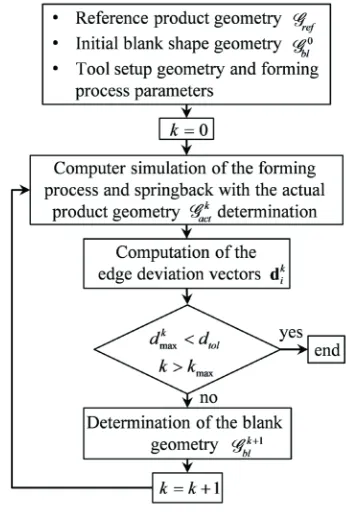
3 NUMERICAL IMPLEMENTATION OF THE PROPOSED BLANK SHAPE OPTIMISATION
The proposed blank shape optimisation method consists basically of a sequence of steps executed iteratively following the flow chart in Fig. 3. Along
with the initial blank shape geometry Gbl0 and
reference product geometry Gref provided, a complete
FE model with the tool geometry and forming process parameters (blank-holder forces, friction conditions, tool movement, etc.) must be specified in order to start the procedure. Since the initial blank shape
geometry Gbl0 plays an important role in attaining
convergence and computational efficiency of the described blank shape optimisation procedure, this geometry should be determined in a way that the edge
geometry Γact0 of the product, obtained by the
corresponding forming process simulation under given process conditions, does not experience too excessive a deviation with respect to the reference
edge geometry Γref. Before starting the procedure the
auxiliary surface Σ
G is determined as explained in
Section 3.1.
Fig. 3. Flow chart of the iterative procedure
The iterative procedure essentially consists
of performing in iteration, say kth iteration, three
consecutive steps. In the first step, the complete technological process, consisting of the forming stage
and subsequent springback stage occurring after removal of the tools, is simulated. This is followed by computing the deviation between the actual product
edge geometry Γactk and its reference edge geometry
Γref, measured with respect to the auxiliary surface
ΣG . The edge deviation computation is performed
in each iteration following the procedure described in Section 3.2. In the last step, the actual blank shape
geometry Gblk is either confirmed as appropriate or,
if the considered edge deviation being found greater than the prescribed tolerance, its further correction
and adjustment to Gblk+1 is required (see Section
3.3). Fulfilment of the tolerance requirements means stopping of the iteration loop, whereas non-fulfilment means that the iteration procedure goes on to the
subsequent (k + 1)th iteration. A detailed description of
how the above general procedure is managed is given in the following sections.
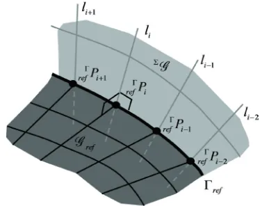
3.1 Determination of the Auxiliary Surface Σ G
The appropriateness of the actual blank shape
geometry Gblk can be established by measuring the
deviation of the actual product edge geometry Γactk
from the reference edge geometry Γref, which can be
done in many ways. Here, the deviation will not be
measured directly with respect to Γref, but indirectly
by making use of an auxiliary virtual surface ΣG
emanating from the reference product edge Γref. This
surface can be generated considering surface topological properties of the reference product
geometry Gref on its edge Γref. Lines li, aligned
along the surface normal vectors ref
i
n at points ref iΓP of the discretised edge, are used, accordingly, as the building basis for the auxiliary surface construction (Fig. 4). To enable numerical control of the actual product edge adequacy this surface is further discretised by quadrilateral sub-domains, yielding
point topology Σ
G . Having those properties, i.e.
emanating from points ref iΓP of the discretised
reference product edge Γref (Γref ⊂ ΣG ) and being
at those points perpendicular to the reference product
geometry Gref, the surface ΣG may be considered in
the iteration process as the target surface, which is to
be attained by the edge points act iΓPk of the actual
product Gactk, as closely as possible.
For a determination of the auxiliary surface ΣG ,
which is computed before starting the optimisation procedure, computation of the surface normal vectors
at points lying on the edge Γref of the reference
product geometry Gref is required.
Fig. 4. Auxiliary surface ΣG determination
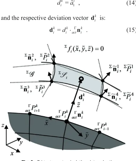
3.2 Determination of the Actual Product Edge Deviation
In the k-th iteration, the deviation dik of individual
edge point act iΓPk of the actual product geometry
k act
G is determined by identifying its distance to the
auxiliary surface ΣG in the direction normal to the
edge. The applied procedure may be divided into three parts. In the first part, the edge normal vector
act iΓnk at point act iΓPk is determined in accordance with the procedure, described in Section 2.3. With
the surface normal vector act ink and tangential vector
act iΓtk computed by Eqs. (8) and (9), respectively, considering surface and edge topology properties of the actual product geometry Gactk, the vector act iΓnk is
determined by Eq. (10).
Fig. 5. Finding surface element ΣS
i on ΣG intersected by a
line collinear with vector act iΓnk
In the second part, intersection with the auxiliary
vector act iΓnk. As the auxiliary surface ΣG is described discretely by quadrilaterals (Fig. 2), it may be assumed
that only one surface element on Σ
G is intersected.
Being actually related to the edge point act iΓPk in the
corresponding determination of the deviation dik, let
us denote this surface by ΣS
i (see Fig. 5) and its nodal
points by ΣP j
ij( = 1,2,3,4).
To enable evaluation of the deviation dik
analytical surface reconstruction of surface SΣ
i ,
ΣF x y z
i( , , ) = 0, is required, which is carried out in
the third part. Apart from the given position vectors
ΣP
ij( = 1,2,3,4)j , the respective surface normal
vectors Σn
ij( = 1,2,3,4)j at those points are also
needed in accordance with Section 2.4. The respective normal vectors’ determination follows the procedure described in Section 2.2.
Although the analytical surface reconstruction of
surface Σ
Si could be done using the global coordinate
system ( , , )x y z , as demonstrated in Section 2.4, it is
better to have the surface Σ
Si representation defined
with respect to a local coordinate system, say ( , , )x y z , which is built by taking the vector triple act iΓtk, act ink, act iΓnk as the system basis and setting the edge point act iΓPk as its origin (Fig. 6), act iΓPk =( , , )0 0 0 . In this way, occurrence of round-off error due to possible computing with large numbers is avoided and accuracy of the computation ensured.
After performing all coordinate transformations
on the position vectors ΣP
ij( = 1,2,3,4)j and
surface normal vectors Σn
ij( = 1,2,3,4)j , as shown
in Section 2.2, and obtaining vectors ΣP
ij and Σnij ,
the geometry of the considered surface element Σ
Si can now be functionally approximated in the local
coordinate system ( , , )x y z . By adopting the same
functional representation as considered in Section 2.4, we have:
Σf x y z z a a x a y
a x y a x
i i i i
i i
( , , ) = ( 1 2 3
4 5 2
− + + +
+ + +
aa y
a x y a xy a x y a x a
i
i i i
i i
6 2 7 2 8 2 9 2 2 10 3 11
+
+ + + +
+ +
yy3 a x yi
12 3 3) = 0
+ . (13)
As in Eq. (12), but expressed in terms of the local coordinate system, the evaluation of the polynomial
coefficients a mmi ( = 1,2,...,12) is based on given
topological requirements fulfilment.
Finally, with the interpolation function
Σf x y z
i( , , ) 0 = fully defined, the deviation dik of
the considered edge point act iΓPk of the actual product
geometry Gactk can be readily determined. Let us first
remember that the coordinate z axis has been chosen
in such a way as to coincide with the edge normal
vector act iΓnk with the origin set at point ΓPik, i.e. act iΓPk =( , , )0 0 0 . Thus, since the deviation is quantified
by the distance measured from point act iΓPk to the
auxiliary surface Σ
G in the direction normal to the
edge, it can be retrieved directly from the functional
representation Σf x y z
i( , , ) 0 = , when taking x y= = 0 in Eq. (13). The established deviation is evidently:
dik =a1i , (14)
and the respective deviation vector dik is:
dik n
ik act ik
d
= ⋅ Γ . (15)
Fig. 6. Edge geometry deviation determination
The deviation of the actual product edge geometry from the reference one, which is established
by the deviation vector set
{ }
dik , determines theappropriateness of the blank shape geometry Gblk
used in the forming process simulation in the given iteration. The maximal shape deviation has been chosen as a measure of this appropriateness:
dmaxk d i N
ik act
=max
{ }
, = 1,2,..., . (16)The deviation of the actual product edge
geometry is computed in each, say, kth iteration. Its
determination requires computation of edge normal
vectors act iΓnk at points lying on the edge Γactk of
the actual product geometry Gactk and finding a
corresponding surface element ΣS
i on the auxiliary
surface ΣG . The respective surface normal vectors
Σn
ij( = 1,2,3,4)j at points of the surface element ΣSi ,
which are also required in computation of the actual product edge geometry deviation, are computed only
once, i.e. after the auxiliary surface ΣG determination
3.3 Blank Shape Geometry Correction
In the case where the convergence criterion is not met, i.e. dmaxk >dtol, a correction of the blank shape
geometry Gblk is required. In our approach, this is
carried out on two levels separately, first, by carrying
out the repositioning of the edge points bl iΓPk, which
is then followed by readjustment of the interior
points bl iPk appertaining to the FE mesh. Correction
of the edge blank shape geometry ΓG
blk is carried out
based on the established deviation vector set
{ }
dik ,Eq. (15), with repositioning of points bl iΓPk applied
in the direction of the edge normal vectors bl iΓnk,
Eq. (10), considering deviation magnitudes dik. The
positions of the points lying on the edge Γblk+1 of the
newly defined blank shape are thus computed by the equation:
bl iΓPk+1=bl iΓPk+dik⋅bl iΓnk. (17) In order to preserve the quality of the simulation in the subsequent iteration, the aspect ratio of the existing FE mesh, used in the description of the blank
shape geometry Gblk, should not be significantly
changed by repositioning of the edge points bl iΓPk.
However, this threat can be efficiently neutralised
by adequate readjustment of the interior points bl iPk
considering the applied edge repositioning, Eq. (17). Numerically, this can be achieved by exposing
the blank having shape geometry Gblk to given
displacement boundary conditions (Fig. 7a) and solving the corresponding boundary value problem, while assuming isotropic linear elastic behaviour. The blank edge nodes are displaced in accordance with the prescribed correction of the blank shape, Eq. (17), while nodes lying on the symmetry planes are subject to symmetric boundary conditions. The result of such computer analysis is the adjusted FE mesh specifying
the blank shape geometry Gblk+1, which will be used in
the subsequent iteration. The adjustment is carried out in accordance with the computed displacement field (Fig. 7b).
4 CASE STUDY - BLANK SHAPE OPTIMISATION
In this section, the developed blank shape optimisation method is validated by considering a particular product with the prescribed edge geometry, manufactured by sheet metal forming (Fig. 8). The product’s geometry, which is originally double planar symmetric by design specification, is characterised by two deep cut outs extending downwards to the cup’s bottom.
a)
b)
Fig. 7. Blank shape geometry correction Gblk →Gblk+1; a) applied displacement boundary conditions, and b) adjustment
of the FE’s mesh
see Halilovič et al. [3] and Vrh et al. [4], has been implemented into ABAQUS/Explicit via the VUMAT
subroutine [32]. The optimisation procedure is carried out using a closed loop Fortran program that has been upgraded by an Abaqus’ Python script to enable display of the optimisation results in each iteration.
After the optimisation blank shape geometry procedure is completed, which is treated in Section 4.2, both the conceived forming process simulation model and the proposed blank shape geometry optimisation procedure are validated experimentally, which is presented in Section 4.3.
4.1 Initial Blank Shape, Reference Product Geometry and Tool Geometry
The geometry of the considered product (referred as the “reference geometry” in this paper) to be obtained by a sheet metal forming process, where a further sheet metal cutting phase is excluded, is shown in Fig. 8a. An aluminium sheet blank of 1.0 mm thickness is used. The cross-section of the corresponding forming tool assembly is shown in Fig. 8b. The forming tool is defined in such a way that its die geometry is determined by the reference product geometry, with a constant clearance of 1.2 mm ensured between the die and the punch, when the tool is in a closed position. In accordance with the assumptions given in Section 2.5, the tool geometry is considered fixed and not subject to possible variation. The design parameters specifying the initial blank shape geometry, used to start the described numerical optimisation blank shape geometry procedure, are displayed in Fig. 8c.
4.2 Determination of Optimal Blank Shape
Determination of the blank shape geometry appropriate for the production of the product, displayed in Fig. 8a, is carried out iteratively following the optimisation procedure, described in Section 3. Thus, a corresponding forming process computer simulation is performed in each iteration, considering the actualised blank shape geometry.
In simulation, the following material and technology process data have been taken into consideration. It is assumed that the product is made from a 1mm thick aluminium sheet exhibiting orthotropic material behaviour, with a Young’s modulus of 72500 MPa, a Poisson’s ratio of 0.3, an initial yield limit of 105 MPa, and coefficients describing orthotropic material properties in relation
to the potential function Hill 48 being: Rxx= 1 0. ,
Ryy= 0 95. and Rxy=0 97. . The yield curve specifying
the hardening plastic behaviour of the given material is plotted in Fig. 9. Since no significant reversed plastic bending occurs during the considered forming process, possible kinematic hardening is neglected and isotropic hardening is assumed.
a)
b)
c)
Fig. 8. Product and forming process geometry design specification; a) product reference geometry, b) forming tool
assembly, and c) initial blank shape geometry
clearance between the die and the punch in a closed position, which is set to 1.2 mm, allows for a potential increase in the sheet thickness during progressing of the punch. For the forming process simulation to be realistic the tribological conditions between the surfaces in contact with one another have to be adequately described. In this investigation the Coulomb friction law is adopted with the friction coefficient between the sheet metal and the tool parts assumed to equal 0.12.
Fig. 9. Yield curve of aluminium sheet
Fig. 10. Numerical model of the forming process
The forming process simulations are based on a FE model, which is conceived in such a way as to cope efficiently with all peculiarities encountered when numerically modelling such a complex problem. Since both the tool and the blank shape geometries
exhibit planar symmetry with respect to the xz and
yz planes and orthotropic material properties are
taken into account, only a quarter of the product can be considered in the model (Fig. 10), with symmetry boundary conditions applied and a given blank-holder force of magnitude 1.3 kN. In the FE model, the tool surfaces are modelled by rigid FEs with a characteristic size of 1.0 mm, while the sheet metal is modelled by deformable reduced integration
quadrilateral shell FEs with a characteristic size of 1.2 mm and with 11 integration points evenly distributed through the shell thickness.
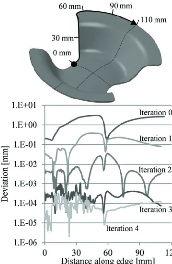
Once the numerical simulation model is completely defined, the steps in the optimisation procedure, given by the flow chart in Fig. 3, can be carried out and the optimal blank shape geometry is achievable iteratively. In Fig. 11, the deviation of the product edge geometry from its reference geometry along the edge contour, as determined by the computer simulation in the considered iteration, is plotted. From these plots it is evident that the developed optimisation procedure is computationally very efficient. Namely, the maximal product edge deviation computed when the initial blank shape is considered in the forming simulation is equal to 3.1 mm. After the first iteration this deviation is reduced to less than 0.3 mm and after two additional iterations to less than 0.001 mm. The shape variation, to which the blank of initial shape geometry is subject when it is optimised using the presented approach, is displayed in Fig. 12.
4.3 Experimental Validation of the Blank Shape Optimisation
In order to validate the developed approach to blank shape geometry optimisation in the investigated case study experimentally, the forming tool parts have been manufactured and assembled in accordance with the design scheme (Fig. 8b). In fact, the forming tool is designed in as simple a way as possible. The punch movement is guided by four cylindrical guides, which also have the function of limiting the punch bottom position. The blank-holder is attached to the tool die by eight sets of bolts and springs under tension so that required blank-holder force is ensured. The blanks used in the experiment are cut out of an aluminium sheet by a water jet cutter.
The experiment was carried out on a HI-KON (model HK250S2) forming press with corresponding measurements of the product edge geometry done by
the 3D measuring machine Brown & Sharpe, Mistral
7-10-7, its accuracy classified as being ±0.004 mm. The product edge geometry was measured at 6 control points along the edge contour (see Fig. 13 for their position).
geometry (Fig. 8c) in order to confirm the physical and numerical appropriateness of the forming process simulation model definition used in the blank shape optimisation procedure. The difference between experimentally (Fig. 13, Exp. initial) and numerically (Fig. 13, Num. initial) obtained product edge geometry deviation is less than 0.20 mm.
Fig. 11. Product edge deviations during iteration process
Fig. 12. Optimised vs. initial blank shape geometry
The difference between the computer simulation and experiment being in the same range as the accuracy of the cutting machine (±0.1 mm), the adequacy of the simulation model can be confirmed. The second experiment was carried out to confirm
the adequacy of the numerically optimised blank shape geometry. As it can be seen from the plots in Fig. 13, the difference between experimentally (Fig. 13, Exp. optimised) and numerically (Fig. 13, Num. optimised) determined product edge geometry is of the same order of magnitude as in the first experiment and is less than 0.22 mm. Therefore, we can confirm that the applied optimisation procedure is appropriate. Photographs of the formed products, produced by the blanks having initial and optimised shape geometry, are displayed in Fig. 14.
Fig. 13. Product edge deviation
Fig. 14. Formed product with initial and optimised blank shape
5 CONCLUSION
corresponding forming process computer simulation. As demonstrated numerically and subsequently validated experimentally, the blank shape optimisation method used here for a specific case study with rather complex product geometry is characterised by computational efficiency and robustness.
6 ACKNOWLEDGMENT
The second author appreciates the support provided in the operation part financed by the European Union, European Social Fund. The operation was implemented within the framework of the Operational Programme for Human Resources Development for the Period 2007 to 2013.
7 REFERENCES
[1] Volk, M., Nardin, B., Dolšak, B. (2011). Application of
numerical simulation in the deep-drawing process and the holding system with segments and inserts. Strojniški vestnik - Journal of Mechanical Engineering, vol. 57, no. 9, p. 697-703, DOI:10.5545/sv-jme.2010.258. [2] Menezes, L.F, Teodosiu, C. (2000). Three-dimensional
numerical simulation of the deep-drawing process using solid finite elements. Journal of Materials Processing Technology, vol. 97, no. 13, p. 100-106, DOI:10.1016/ S0924-0136(99)00345-3.
[3] Fan, J.P., Tang, C.Y., Tsui, C.P., Chan, L.C., Lee, T.C. (2006). 3d finite element simulation of deep drawing with damage development. International Journal of Machine Tools and Manufacture, vol. 46, no. 9, p. 1035-1044, DOI:10.1016/j.ijmachtools.2005.07.044.
[4] Vrh, M., Halilovič, M., Starman, B., Štok, B., Comsa,
D., Banabic, D. (2011). Earing prediction in cup drawing using the bbc2008 yield criterion. AIP Conference Proceedings, vol. 1383 no.1, p. 142-149, DOI:10.1063/1.3623604.
[5] Halilovič, M., Vrh, M., Štok, B. (2009). Nice-an explicit
numerical scheme for efficient integration of nonlinear constitutive equations. Mathematics and Computers in Simulation, vol. 80, no. 2, p. 294-313, DOI:10.1016/j. matcom.2009.06.030.
[6] Vrh, M., Halilovič, M., Štok, B. (2010). Improved
explicit integration in plasticity. Inernational Journal of Numerical Methods in Engineering, vol. 81, no. 7, p. 910-938.
[7] Vrh, M., Halilovič, M., Štok, B. (2011). The evolution
of effective elastic properties of a cold formed stainless steel sheet. Experimental Mechanics, vol. 51, p. 677-695, DOI:10.1007/s11340-010-9371-1.
[8] Vrh, M., Halilovič, M., Starman, B., Štok, B. (2011). A
new anisotropic elasto-plastic model with degradation of elastic modulus for accurate springback simulations. International Journal of Material Forming, vol. 4, no. 2, p. 217-225, DOI:10.1007/s12289-011-1029-8.
[9] Koc, P., Štok, B. (2008). Usage of the yield curve in numerical simulations. Strojniški vestnik - Journal of Mechanical Engineering, vol. 54, no. 12, p. 821-829. [10] Batoz, J.L., Duroux, P., Guo, Y.Q., Detraux, J.
M. (1989). An efficient algorithm to estimate the large strains in deep drawing. Proceedings of the NUMIFORM, p. 383-388.
[11] Batoz, J.L., Guo, Y.Q. (1997). Analysis and design of sheet forming parts using a simplified inverse approach. COMPLAS V, Barcelona, p. 178-185.
[12] Batoz, J.L., Guo, Y.Q., Mercier, F. (1998). The inverse approach with simple triangular shell elements for large strain predictions of sheet metal forming parts. Engineering Computations, vol. 15, no. 7, p. 864-892, DOI:10.1108/02644409810236894.
[13] Chung, K., Richmond, O. (1992). Ideal Forming-I. Homogeneous deformation with minimum plastic work. International Journal of Mechanical Sciences, vol. 34, no. 7, p. 575-591, DOI:10.1016/0020-7403(92)90032-C.
[14] Chung, K., Richmond, O. (1992). Ideal Forming-II. Sheet forming with optimum deformation. International Journal of Mechanical Sciences, vol. 34, no. 8, p. 617-633, DOI:10.1016/0020-7403(92)90059-P.
[15] Azaouzi, M., Belouettar, S., Rauchs, G. (2010). A numerical method for the optimal blank shape design. Materials and Design, vol. 32, no. 2, p. 756-765, DOI:10.1016/j.matdes.2010.07.027.
[16] Azaouzi, M., Naceur, H., Delamoziere, A., Batoz, J.L., Belouettar, S. (2008). An heuristic optimization algorithm for the blank shape design of high precision metallic parts obtained by a particular stamping process. Finite Elements in Analysis and Design, vol. 44, no. 14, p. 842-850, DOI:10.1016/j.finel.2008.06.008.
[17] Naceur, H., Guo, Y.Q., Batoz, J.L. (2004) Blank optimization in sheet metal forming using an evolutionary approach. Journal of Materials Processing Technology, vol. 151, no. 1-3, p. 183-191, DOI:10.1016/j.jmatprotec.2004.04.036.
[18] Park, S.H., Yoon, J.W., Yang, D.Y., Kim, Y.H. (1999) Optimum blank design in sheet metal forming by the deformation path iteration method. International Journal of Mechanical Sciences, vol. 41 no. 10, p. 1217-1232, DOI:10.1016/S0020-7403(98)00084-8. [19] Yeh, F.H., Wu, M.T., Li, C.L. (2007). Accurate
optimization of blank design in stretch flange based on a forward inverse prediction scheme. International Journal of Machine Tools and Manufacture, vol. 47, no. 12-13, p. 1854-1863, DOI:10.1016/j. ijmachtools.2007.04.002.
[20] Lin, C.T., Kwan, C.T. (2009). Application of abductive network and fem to predict the optimal blank contour of an elliptic cylindrical cup from deep drawing. Journal of Materials Processing Technology, vol. 209, no. 3, p. 1351-1361, DOI:10.1016/j.jmatprotec.2008.03.042. [21] Parsa, M.H., Pournia, P. (2007). Optimization of initial
method. Finite Elements in Analysis and Design, vol. 43, no. 3, p. 218-233, DOI:10.1016/j.finel.2006.09.005. [22] Pegada, V., Chun, Y., Santhanam, S. (2002). An
algorithm for determinig optimum blank shape for the deep drawing of the alluminium cups. Journal of Materials Processing Tehnology, vol. 125-126, p. 743-750, DOI:10.1016/S0924-0136(02)00382-5.
[23] Son, K., Shim, H. (2003). Optimal blank shape design using the initial velocity of the boundary nodes. Journal of Materials Processing Technology, vol. 134, no. 1, p. 92-98, DOI:10.1016/S0924-0136(02)00927-5.
[24] Hamammi, W., Padmanbhan, R., Oliveira, M.C., BelHadjSalah, H., Alves, J.L., Menzes, L.F. (2009), A deformation based blank design method for formed parts. International Journal of Mechanics and Materials in Design, vol. 5, no. 4, p. 303-314, DOI:10.1007/s10999-009-9103-9.
[25] Fazli, A., Arezoo, B. (2012). A comparison of numerical iteration based algorithms in blank optimization. Finite Elements in Analysis and Design, vol. 50, p. 207-216, DOI:10.1016/j.finel.2011.09.011.
[26] Sattari, H., Sedaghati, R., Ganesan, R. (2007). Analysis and design optimization of deep drawing process part
ii: Optimization. Journal of Materials Processing Technology, vol. 184, no. 1-3, p. 84-92, DOI:10.1016/j. jmatprotec.2006.11.008.
[27] Padmanabhana, R., Oliveiraa, M.C., Baptistaa, A.J., Alvesb, J.L., Menezesa, L.F. (2009). Blank design for deep drawn parts using parametric nurbs surfaces. Journal of Materials Processing Technology, vol. 209, no. 5, p. 2402-2411, DOI:10.1016/j. jmatprotec.2008.05.035.
[28] Shim, K., Son, H., Kim, K. (2000). Optimum blank shape design by sensitivity analysis. Journal of Materials Processing Technology, vol. 104, no. 3, p. 191-199, DOI:10.1016/S0924-0136(00)00556-2. [29] Cafuta, G., Mole, N., Štok, B. (2012). An enhanced
displacement adjustment method: Springback and thinning compensation. Materials and Design, vol. 40, p. 476-487, DOI:10.1016/j.matdes.2012.04.018. [30] SIMULIA. (2008). ABAQUS/Explicit, 6.8-1, Simulia,
Providence.
[31] SIMULIA. (2008). ABAQUS/Standard, 6.8-1, Simulia, Providence.