in the population sciences published by the Max Planck Institute for Demographic Research Konrad-Zuse Str. 1, D-18057 Rostock·GERMANY www.demographic-research.org
DEMOGRAPHIC RESEARCH
VOLUME 18, ARTICLE 11, PAGES 311-336
PUBLISHED 23 APRIL 2008
http://www.demographic-research.org/Volumes/Vol18/11/ DOI: 10.4054/DemRes.2008.18.11
Research Article
Correlated mortality of siblings in Kenya:
The role of state dependence
D. Walter Rasugu Omariba
Fernando Rajulton
Roderic Beaujot
c
°2008 Omariba, Rajulton & Beaujot.
1 Introduction 312
2 Infant death clustering: An overview 313
3 Analytic model 316
4 Data 319
4.1 Clustering of children and infant deaths by family 320
4.2 Description of variables 321
5 Results 323
6 Discussion and conclusion 329
7 Acknowledgements 332
Correlated mortality of siblings in Kenya:
The role of state dependence
D. Walter Rasugu Omariba1
Fernando Rajulton2 Roderic Beaujot3
Abstract
Random-effect models have been useful in demonstrating how unobserved factors are re-lated to infant or child death clustering. Another potential hypothesis is state dependence whereby the death of an older sibling affects the risk of death of a subsequent sibling. Probit regression models incorporating state dependence and unobserved heterogeneity are applied to the 1998 Demographic and Health Survey (DHS) data for Kenya. We find that mortality risks of adjacent siblings are dependent: a child whose preceding sibling died is 1.8 times more likely to die. After adjusting for unobserved heterogeneity, the death of the previous child accounts for 40% of child death clustering. Further, elimi-nating state dependence would reduce infant mortality among second- and higher-order births by 12.5%.
1Health Information & Research Division, Statistics Canada, 100 Tunney’s Pasture Driveway, R.H. Coats
Building 24B, Ottawa, Ontario K1A 0T6, Canada. Tel: 613-951-6528. Fax: 613-951-3959. Email: [email protected]
2Population Studies Centre, Department of Sociology, University of Western Ontario, London, Ontario N6A
5C2, Canada.
3Population Studies Centre, Department of Sociology, University of Western Ontario, London, Ontario N6A
1. Introduction
Since Das Gupta (1990) suggested the concept of “death clustering”, demographers have been preoccupied with understanding why deaths concentrate in certain families. Death clustering has been understood as a phenomenon in which greater heterogeneity exists in the distribution of child deaths than would be expected if deaths were distributed ran-domly. Additionally, it has been viewed as what is left unexplained after the observed correlates are controlled, and is thus attributed to unobserved or unobservable genetic, behavioral and environmental factors related to mortality (Guo 1993; Ronsmans 1995; Das Gupta 1997). It is also sometimes viewed as the correlation of survival outcomes among siblings.
Studies of infant and child mortality in less developed countries mainly use maternal retrospective birth histories data from DHS. The main approaches to examine death clus-tering, therefore, essentially view it as a way of accounting for the correlation in mortality risks among siblings (Zenger 1993). In the literature, the major approach to the study of death clustering is to examine whether residual variation remains after accounting for observed determinants of mortality by using random effects models (Sastry 1997; Sear et al. 2002). The random effects parameter is used to measure the effect of unobserved factors on the risk of death and to estimate the extent to which the risks of death in a group are correlated. Unobserved heterogeneity, however, is not the only mechanism associated with familial child death clustering.
Drawing on recent work in this area (Arulampalam & Bhalotra 2006), this study ex-amines the causal process triggered by the death of an older sibling that in turn increases the risk of death of the next child in the family. This is the well known process of state dependence. The paper in particular attempts to clarify the concept of death clustering and brings out the fact that it needs to be closely associated, and therefore examined, with the sequence of births and deaths in a family. Earlier analyses have ignored this impor-tant idea, either in the clarification of the concept or in the analytical approaches used to examine the presence and extent of death clustering. As further elaborated below, the sequences of births and deaths can be analyzed through models that also incorporate un-observed heterogeneity. Using these models, we estimate one parameter to capture state dependence and another to measure the variance associated with unobserved factors in the risk of death. The analysis considers only infant deaths, that is, deaths that occurred between birth and completed age of 11 months. The mother is considered as constituting the family level in the subsequent analyses.
total fertility rate of 4.9 in 2003 (Central Bureau of Statistics [CBS], Ministry of Health (MOH), & ORC Macro 2004).
2. Infant death clustering: An overview
Studies that conceptualize the issue as an expression of unmeasured heterogeneity ex-tend standard logistic regression techniques to allow for correlation by assuming that the level of mortality risk varies among families and follows a probability distribution. This assumption leads to the random intercept model which describes the probability of death, conditional on the random intercept, as a nonlinear function of possible family- or community-level explanatory variables. The underlying index, however, is linear in its arguments. It is also possible to assume there are several levels in the data or that coef-ficients of the explanatory variables are also random, thus producing a more complicated correlation structure (Zenger 1993; Raudenbush & Bryk 2002). Because the random in-tercept models assume an exchangeable correlation structure, all siblings are associated equally. Zenger (1993) has demonstrated that death clustering may not be captured by random effects models in part because of the restrictive assumptions of the model. In particular, the number of children and the number of deaths in most families is relatively small to yield significant variation. A second approach considers child death clustering as a measure of excess observed versus expected deaths (Ronsmans 1995; Das Gupta 1997). This approach uses count models to estimate the expected distribution of deaths from the observed child deaths in families. Count models, however, assume that the probability of a child death is the same for all families in a given group and do not permit one to examine whether interfamily variation in mortality is related to the experience of close siblings (Zaba & David 1996).
The concept of death clustering inherently implies the survival status of preceding children, that is, the survival of a younger child in the family depends on whether an older sibling has died. For instance, Zenger (1993) found that in Bangladesh familial associa-tion in the risk of neonatal death was strongest for siblings of adjacent birth orders. The effects of survival status of the previous child can be explained in three important ways. First, a child’s death truncates the interval to the subsequent birth, which is in turn asso-ciated with the maternal depletion syndrome that can lead to preterm and low birthweight children and pregnancy complications. Second, parents may make a deliberate decision to replace the dead child, the so-called replacement hypothesis (e.g., LeGrand et al. 2003). Third, an obvious but a largely missing hypothesis in demographic literature is mater-nal depression. Depression is associated with negative pregnancy outcomes including preterm delivery, low birthweight and small-for-gestational-age babies all of which are significant risk factors for child death (Steer et al. 1992). Because maternal depression seems independent of birth interval, it is possible to isolate it from the other two mech-anisms. Although it is difficult to precisely determine what mechanism is operating in a given situation, the exercise is important for selecting between policy options. On the one hand, if its effect reflects the birth spacing mechanism, improving availability and use of contraception would reduce death clustering, a straightforward policy response. On the other hand, policy options responding to depression and replacement mechanisms are less certain.
Thus, the concept of death clustering implies examining the survival status of an in-dex child as dependent on the survival status of previous children. If the survival status of an index child is dependent on the survival status of the immediately previous child only, it is said to be of the first-order Markov effect. Studies examining both unobserved heterogeneity and state dependence, for example, in econometric studies of unemploy-ment (Heckman 1981; Wooldridge 2005; Stewart 2007) or even in demographic studies of death clustering (Arulampalam & Bhalotra 2006; Bhalotra & van Soest 2007) generally consider the first-order Markov effect. The concept of death clustering, however, involves more than that. In general, one can ask how many deaths should take place in a family to say for certain that there is “death clustering” in the family. If only one infant dies, we may not attribute clustering effect to that context. Should there be two or three or four or how many infants should die then? Is there a threshold point that we can use to clarify the concept of interest? This specific point has not been addressed in previous research as far as we know. There is therefore a need to explicitly address the question by examining it through a higher-order Markov effect in the model. We shall return to this point later in the section on model building.
characteristics (Zaba & David 1996; Das Gupta 1997). Das Gupta (1997) found that in India the variation between the observed and expected child deaths in the lower economic-status groups was greater than in the higher economic-economic-status groups. Similarly, significant clustering was found among uneducated women than among educated women. The study suggested that unobserved factors associated with death clustering are more positively associated with socioeconomic conditions and education level. Certain households may suffer from unusual adverse conditions such as insufficient economic resources, health conditions, or access to medical care. Siblings share the same household environmental conditions and hence, any risks associated with these conditions such as lack of sanitation and unsafe water supply, affect all of them. Also, risks associated with family behavior and child care practices including infant feeding, use of health facilities, and general standards of hygiene are likely shared by all siblings (Curtis et al. 1993; Pebley, Goldman & Rodriguez 1996). Cultural practices in certain population sub-groups could also lead to a concentration of deaths in those sub-groups. For instance, in highly male-oriented and patriarchal societies, death clustering could be due to an attempt to remove girls through differential childcare (Das Gupta 1997).
Death clustering is also likely to be more pronounced among women with higher par-ities (Zaba & David 1996). Besides shared genetic characteristics that could be operating in such situations, children in big families may face competition for resources and be more likely to suffer infectious diseases because of crowding in the household (e.g., Grib-ble 1993). As family size increases, not only are family resources stretched increasing the risk of malnutrition, but overcrowding makes contagious disease to spread faster (Aaby 1992). Illnesses are also more likely to be fatal in the presence of malnutrition.
Death clustering has also been attributed to lack of ’maternal competence’ in child-care. For instance, Das Gupta (1990) concluded from participant observation that women who experienced multiple child deaths were often less resourceful and less organized in caring for their surviving children and in running the household even when compared with women in households with similar socioeconomic status. In relation to child care, such women were poor at making effective home diagnoses of their children’s symptoms and taking active steps to help them. Because a large majority of child illnesses are han-dled within the home, less resourceful mothers are disadvantaged. However, there is a practical problem in measuring a mother’s resourcefulness because in any community, the proportion of mothers who are less resourceful and unskilled in childrearing is likely to be small. The distribution of deaths would therefore not be random because only few families contribute to the total deaths that occur in the community.
young do not pass on their unfavorable genes. Genetic factors and other familial effects, however, are not measured in social surveys. It is difficult therefore to uniquely identify which of the factors are responsible for death clustering. Other important biological fac-tors include the tendency of certain mothers to have babies of low birthweight, or to suffer difficult deliveries, or lactational failure (Knodel & Hermalin 1984).
3. Analytic model
There are two main issues associated with modeling siblings’ survival outcomes. First, the selected approach should be able to handle state dependence because the survival sta-tus of an older child could impact that of the younger one. Second, there is the need to model unobserved heterogeneity as well because of between family variation in childcare practices, access to healthcare, and other unobserved characteristics. Consequently, bi-nary probit models incorporating an unobserved heterogeneity term and a lag effect to capture state dependence are used to examine infant mortality. The inclusion of a lag pa-rameter implies that the data are ordered sequentially and therefore the model is dynamic because sequencing incorporates a time dimension.
The main interest of the model is to establish whether the death of an older sibling
(j −1)in family ihas an influence on the survival status of the next child (j =index child)1. Lety∗
ij be the latent propensity for the occurrence of infant death. The latent
equation for the random effects dynamic probit model is specified as
y∗i,j=x0ijβ+γyij−1+αi+uij (1)
(i = 1,2, ..., N; j = 1,2, ..., ni) wherexdenotes a vector of observable child- and
family-level characteristics,βis a vector of parameter estimates associated withx,γis the lag parameter capturing the influence of the death of the previous child on that of the next one, andαi are unobserved family specific random effects, anduij N(0, σ2u). The
standard random effects model assumesαi is uncorrelated with the included covariates
xij2. The binary outcome variable (in this case, infant death) is given by:
1Demographic and health surveys use a multi-stage cluster sampling approach. The sampling clusters therefore
represent another hierarchy in the data that needs to be adjusted for. These clusters, however, are created for sampling and survey administration purposes and may have no substantive meaning in relation the research issue (see Montgomery & Hewett 2005). For this reason and the fact that it is difficult to interpret the cluster effect on the survival experience of children born at different times and the limitations of the program redprob used here (see below) it is not incorporated in the models.
2But this assumption can be relaxed by assuming a relationship between and the family-specific means ofx
yij =
½
1 ify∗ ij≥0
0 otherwise (2)
UsuallyN is large, butniis typically small (here denoting the number of children in a
family). Ifαi = 0, it means that unobserved family-level factors have no effect on the
probability of child death. Similarly, ifγ= 0, it implies that the probability of the index child dying is independent of an older child’s death. Its estimate is an average over the number of children and the time period considered. The standard random effects model also assumesαiis uncorrelated withxij. The composite error termvij =αi+uijwill
be usually correlated due to family-specificαi, and the model assumes equi-correlation
between thevijfor any two children, which is given by
λ= Corr(vij, vik) = σ
2
α
σ2
α+σ2u
, j, k= 1,2, ..., ni, j6=k (3)
With these specifications, the probability of death for an infantjof motheri, givenαi, is
given by
P[yij |xij, yij−1, αi] = Φ[(x0ijβ+γyij−1+αi)(2yij−1)] (4)
whereΦdenotes the cumulative distribution function of the normal distribution. And, droppingxfor convenience the observed sequence of binary outcomes is given by:
P(yin, ..., yi2, yi1|αi) = P(yin|yin−1, αi)...P(yi2|yi1, αi) P(yi1|αi) (5)
Equations (1) and (5) make it clear that this is a transition model based on the Markov assumption that the probability of infant death depends on the survival status of an im-mediately previous child. The number of previous births and deaths determining the transition probability is called theorderof the Markov chain model. The model above is a first-order Markov model and assumes that conditional onyij,xijandαi, the deaths of
older siblings other than the immediately preceding child has no effect onyij.
With the data arranged in a sequence, it is possible that the death of a younger sibling occurred before that of the older one. This is more likely to happen for child than infant mortality because of the longer period of observation. If the death of a younger child preceded that of an older child, then the Markovian assumption will be violated. Our data, however, does not have any such observations.
The inclusion of the lagged term,yij−1in equations (1) and (4), however, introduces a bias because it is undefined for all firstborns (Hsiao 2003). In particular, as equation (5) shows, the model requires a specification forP(yi1 | αi). Some studies therefore
also to ensure the event of interest corresponds closely to the observed characteristics and conditions at survey date. As a consequence, the start of the sample is not the same as the start of the stochastic process that is being examined. Becauseαiis family-specific, it
will appear both in the equation foryij andyij−1. The initial condition,yij, is therefore
correlated withαi andγwould be overestimated (Fatouhi 2005). The estimation of the
model therefore requires an assumption regardingyi1and its relationship with αi. An
assumption leading to the simplest form of model for estimation would be to consider the initial condition to be exogenous. Such an assumption can be made if the start of the process coincided with the start of the observation period for each respondent. This assumption is reasonable in the case of employment data where everyone starts without employment. In the current case, however, endogeneity of the survival status of the first-born is an issue because maternal frailty affects the health of both the first and subsequent children. Hsiao (2003) suggested that the initial conditions problem can be avoided if the “number of time points” of the panel are large. This situation is also not satisfied in our sample because, as noted earlier,nihere denoting the number of a woman’s children is
always finite. See Heckman (1981), Wooldridge (2005), Hsiao (2003), and Arulampalam & Bhalotra (2006) for more details on the initial conditions problem.
In most situations, the initial conditions would be correlated with theαi, and therefore
the estimator will be inconsistent and will overestimateγ, thus overstating the importance of state dependence. To correct for this bias, the approach proposed by Heckman (1981) involves specifying a linearized reduced form equation for the initial conditionyi1(here, the first child in each family):
y∗
i1=zi01π+θαi+ui1 (6)
wherezi1is a vector of exogenous variables (for example, pre-sample characteristics of respondents) which can include time invariant components ofxijandθαi(withθ >0) is
correlated withαi, but uncorrelated withuijforj ≤2. Equation (6) ensures that the risk
of death of the firstborns of each family is also included in the model, and both equations (1) and (6) jointly specify a complete model for infant mortality. This model would give consistent estimates of the effect of the survival status of the immediate preceding sibling on the death of an index child.
The Heckman approach gives the joint probability of the observed binary sequence for familyi, givenαi, as
P(yi1, yi2, ..., yini|xi, zi1, αi) = Φ{(zi1π+θαi)(2yi1−1)} ·
· ni Y
j=2
Φ©(x0
ijβ+γyij−1+αi)(2yij−1)
ª
Given that the outcome variable is binary, a normalization is required to identify the pa-rameters. By convention, this is set asσ2
u= 1. Under this normalization,σα2 =λ(1−λ)
- see Equation (3). Therefore, the individual likelihood function for familyibecomes:
Y
i
Z
α∗
h
Φ©(z0i1π+θσαα∗) + (2yi1−1)
ª
·
· ni Y
j=2
Φ©(x0
ijβ+γyij−1+σαα∗)(2yij−1)
ª
dF(α∗)i (8)
whereF is the distribution function ofα∗= α σα
The joint random-effects dynamic probit model taking account of initial conditions is non-standard and therefore cannot be estimated using the routines available in standard statistical software. Stewart (2006, 2007) has written an ado (automatic do) file for Stata, calledredprob.ado, for fitting the random effects dynamic probit model. This program uses the maximization procedures in Stata and the Gaussian quadrature to approximate the integral in the individual likelihood functionLi(Equation (8)) (StataCorp 2006). The
results from the random effects dynamic probit model presented below are based on spec-ifying 24 quadrature points in the procedure.3
4. Data
The 1998 Kenya DHS used in this study was the third in the series of similar surveys un-dertaken in the country. The survey was based on individual interviews of women in the reproductive ages, 15-49 years and their partners in the sampled households. The survey successfully interviewed 7,881 of 8,233 eligible women from 8,380 sampled households. Of the 7,881 women who were successfully interviewed, 5,717 had given birth to at least one child yielding a total of 23,351 children. The analysis, however, excluded 62 children who were born on the month of interview because their mortality experience is unknown. Further, we dropped each second firstborn twin (57 children) so that each family has one first observation. The analysis is based on 23,232 children (n) from 5,695 families (N). A detailed description of the survey including sampling procedure, data quality, and descriptive information on infant and child mortality, fertility, family planning and
house-3Another ado file for Stata, calledrelogm1.ado, written by Arulampalam and Bhalotra (2006) can also be used to
hold information among others is available in the survey report (National Council for Population and Development, Central Bureau of Statistics & Macro International 1999).
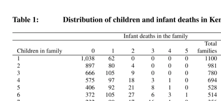
4.1 Clustering of children and infant deaths by family
Table 1: Distribution of children and infant deaths in Kenya, DHS1998
Infant deaths in the family Percent of Total total total Children in family 0 1 2 3 4 5 families children of deaths
1 1,038 62 0 0 0 0 1100 4.7 3.9
2 897 80 4 0 0 0 981 8.4 5.5
3 666 105 9 0 0 0 780 10.1 7.7
4 575 97 18 3 1 0 694 11.9 9.1
5 406 92 21 8 1 0 528 11.4 10.1
6 372 105 27 6 3 1 514 13.3 12.1
7 232 90 17 16 1 0 356 10.7 11.0
8 157 72 25 12 5 2 273 9.4 11.7
9 131 57 20 9 2 3 222 8.6 9.2
10-15 92 68 42 22 17 6 247 11.4 19.9
Total families 4,566 828 183 76 30 12 5,695 100 100 Percent total children 70.5 19.2 5.7 2.7 1.2 0.5 100
Percent of total deaths 0 51.6 22.8 14.2 7.5 3.9 100
The descriptive results in Table 1 serve as a basis for determining whether there is need to control for familial correlation of mortality risks. The table is interpreted in two complementary ways: the percentage of children who belong to families with a given number of children and the percentage of deaths occurring to families with a given number of infant deaths. Only 5 percent of the total 23,232 children come from families with one child and about 87 percent of the children belong to families with three or more children. Of the families with 10-15 children, 139 families had 10, 54 families had 11, 37 had 12, 12 had 13, 3 had 14, and 2 had 15 children each for a total of 2,656 children. Only 37.6 percent of the families have five or more children, and yet these children make up about two-thirds of total children.
with three or more child deaths. Slightly less than 1 percent of the families contribute four or more deaths; together they account for about 11 percent of all deaths. These results therefore indicate that there is substantial clustering of child deaths in certain families as a majority of families did not experience any death.
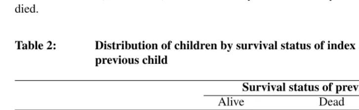
A cross-classification of infant deaths (yij) by survival status of immediately previous
child (yij−1) in Table 2 corroborates this point. About twenty two percent of the dead
index children are preceded by siblings who also died in infancy (row percentage). The observedconditional probabilitiesp1andp0of an infant death given that his/her imme-diately previous sibling died or survived respectively can be obtained from Table 2 (see column percentages):
p1= P(yij = 1|yij−1= 1) = 0.179 and p0= P(yij = 1|yij−1= 0) = 0.059
This suggests that the probability of infant death in Kenya is higher by 0.12 (0.179-0.059) if the preceding sibling died in infancy. The result can also be interpreted as a ratio, that is, a child is 3.03 (0.179/0.059) times more likely to die in infancy if its preceding sibling died.
Table 2: Distribution of children by survival status of index and previous child
Survival status of previous child
Alive Dead Totaln
Survival status of index child Row Percentages
Alive 92.7 7.3 16,334
Dead 78.3 21.7 1,203
Column Percentages
Alive 94.1 82.1
Dead 5.9 17.9
Totaln 16,082 1,455
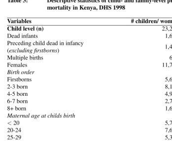
4.2 Description of variables
The main independent variable in this study is the survival status of the immediate preceding sibling (yij−1). Just as in the outcome measure it takes the value 1 if the
immediate preceding sibling died in infancy and 0 otherwise. Where the index child was a twin or triplet, care was taken to ensure that the survival status of the preceding child is the same for all of them. Similarly, when the previous birth was a multiple birth,yij−1 takes the value 1 if any of the children of a multiple birth died in infancy and 0 otherwise. The death of only one of the children of a multiple birth is not likely to lead to the cessation of breastfeeding and hence a shortened succeeding birth interval. Nonetheless, maternal health status may be compromised through its depressive effects.
We control for five child-level variables: sex, whether the child is of a multiple birth, birth order, maternal age at child’s birth, and birth interval. Birth order affects infant death through primaparity, depletion of maternal physiological system from repeated pregnan-cies and siblings’ competition for household resources. The effects of maternal age at the birth of the child could also include primaparity and maternal physiological state (Miller 1993; Alam 2000). The preceding birth interval, however, needs special consideration be-cause of its close association with the preceding child’s survival status. Having these two variables in a model is synonymous with including both the ultimate and the proximate cause (Arulampalam & Bhalotra 2006). The death of a previous child has its impact on the index child’s risk of dying mainly through a shortened birth interval. Further, birth interval is potentially a choice variable if use of contraception is involved. Short birth intervals also imply that most births are concentrated within a certain age range of the mother, creating a compound effect of both age and spacing. It seems therefore reason-able not to include the preceding birth interval. We, however, include the birth interval in the model to assess the extent of the impact of the preceding child’s survival status on the death of the index child after controlling for birth interval. If the effect of the preced-ing child survival status remains strong with birth intervals controlled for, it will suggest the presence of other unexplored mechanisms such as depression. This can be checked by comparing two models, one with and the other without the birth interval. Following extant research children are grouped into either of these categories: born less than 19, 19-35, or 36 or more months after the preceding sibling (e.g., Zenger 1993).
family-level variables namely, maternal and paternal education, religion, ethnicity, and mother’s birth cohort.
Maternal education is a proxy for a host of unmeasured factors such as mother’s child-care skills, domestic management of child illness, household power dynamics and effec-tive use of modern health services. Paternal education is considered mainly as an indicator of household socioeconomic status (e.g., Caldwell 1994; Desai & Alva 1998). Both eth-nicity and religion are included to capture socio-cultural influences on infant mortality. Ethnicity indicates cultural childcare practices including feeding, breastfeeding, and use of health services, which are not directly measured or are not measured for all children. Religion measures beliefs, norms and value orientations including attitudes toward child illness and appropriate responses (e.g., Gregson et al. 1999). The birth cohort of the mother can capture changes in mortality risks across time because our data includes chil-dren born during different time periods. The description of these variables is presented in Table 3.
5. Results
Four probit models that incorporate state dependence and unobserved heterogeneity are estimated. The first includes only state dependence; the second adds child-level factors, whereas the third includes family-level factors. Model 4 which includes a control for birth interval tests for its impact on the relationship between the death of the preceding child and infant death. The covariates in the equation for the firstborns include family-level characteristics as well as the sex of the index child.
For each estimated model, theredprob.adoprogram produces three sets of parameters: the first is for thepooled probit modelforj >1only (that is, for all subsequent children). The pooled probit model ignores the correlation among children within families. The second set of parameters is forj= 1only, that is, a model of initial conditions. And, the third is for the full probit model that combines both. The results from the random effects probit model are presented in Table 4. The results from the pooled probit model are not reported, but are available on request from the first author. The results from the random effects probit model cannot be directly compared with the results from the pooled probit model because they use different normalizations: While the former uses a normalization ofσ2
u = 1, the pooled probit model usesσv2 = 1. For comparisons, the random effects
probit model estimates should be rescaled by an estimate ofσu/σv = √
Table 3: Descriptive statistics of child- and family-level predictors of infant mortality in Kenya, DHS 1998
Variables # children/ women Percentage
Child level (n) 23,232
Dead infants 1,605 6.9
Preceding child dead in infancy
1,455 8.3
(excluding firstborns)
Multiple births 613 2.6
Females 11,710 49.6
Birth order
Firstborns 5,695 24.5
2-3 born 8,171 35.2
4-5 born 4,991 21.5
6-7 born 2,720 11.7
8+ born 1,655 7.1
Maternal age at childs birth
<20 5,715 24.6
20-24 7,656 33.0
25-29 5,369 23.1
30-34 2,996 12.9
≥35 1,496 6.4
Preceding birth interval (excluding firstborns)
<19 months 2,926 16.7
19-35 months 9,414 53.7
≥36 months 5,197 29.6
The results of Model 1 with state dependence only (the parameterγ) show that the death of an immediate older sibling has a positive and highly significant effect on the conditional probability of infant death. The partial effect ofyij−1onP(yij = 1)can be
found from the estimates of counterfactual outcome probabilities, takingyij−1as fixed at 0 and 1 and evaluated atxij=x. The resulting probabilities (p0andp1from the model)
can be interpreted as average partial effects (APE) by taking the difference between them or as predicted probability ratios (PPR) by taking the ratio of the two values (Stewart 2007: 522). The conditional probabilities estimated by the model are given asp1= 0.108
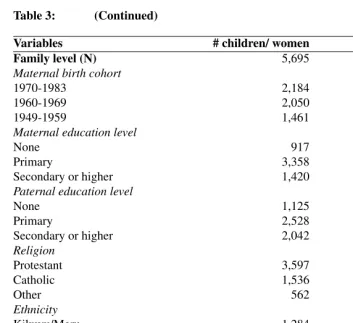
Table 3: (Continued)
Variables # children/ women Percentage
Family level (N) 5,695
Maternal birth cohort
1970-1983 2,184 38.3
1960-1969 2,050 36.0
1949-1959 1,461 25.7
Maternal education level
None 917 16.1
Primary 3,358 59.0
Secondary or higher 1,420 24.9
Paternal education level
None 1,125 19.8
Primary 2,528 44.4
Secondary or higher 2,042 35.9
Religion
Protestant 3,597 63.2
Catholic 1,536 27.0
Other 562 9.9
Ethnicity
Kikuyu/Meru 1,284 22.5
Kamba 603 10.6
Kalenjin 1,021 17.9
Kisii 419 7.4
Luhya 814 14.3
Luo 731 12.8
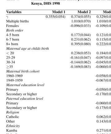
Table 4: Results from random effects probit models for infant mortality in Kenya, DHS 1998
Variables Model 1 Model 2 Model 3 Model 4
γ 0.355(0.054) 0.374(0.055) 0.329(0.055) 0.266(0.056)
Multiple births 1.010(0.070) 1.010(0.070) 1.020(0.070)
Females -0.096(0.033) -0.109(0.033) -0.106(0.033)
Birth order
4-5 born 0.177(0.044) 0.121(0.046) 0.084(0.046)
6-7 born 0.231(0.062) 0.115(0.063) 0.042(0.064)
8+ born 0.395(0.080) 0.222(0.082) 0.120(0.083)
Maternal age at childs birth
<20 0.238(0.053) 0.184(0.053) 0.135(0.054)
25-29 -0.161(0.047) -0.097(0.048) -0.040(0.049)
30-34 -0.144(0.062) -0.045(0.063) 0.063(0.065)
≥35 -0.169(0.083) -0.060(0.085) 0.098(0.088)
Maternal birth cohort
1960-1969 -0.058(0.057) -0.081(0.057)
1949-1959 -0.067(0.059) -0.107(0.060)
Maternal education level
Primary -0.050(0.047) -0.044(0.047)
Secondary or higher -0.170(0.071) -0.185(0.072)
Paternal education level
Primary -0.060(0.051) -0.065(0.051)
Secondary or higher -0.175(0.062) -0.188(0.062)
Religion
Catholic 0.062(0.042) 0.063(0.042)
Other 0.143(0.075) 0.147(0.076)
Ethnicity
Kamba 0.271(0.077) 0.281(0.078)
Kalenjin 0.150(0.067) 0.144(0.067)
Kisii 0.067(0.090) 0.069(0.091)
Luhya 0.386(0.068) 0.377(0.068)
Luo 0.797(0.066) 0.813(0.067)
Mijikenda/Other 0.176(0.080) 0.179(0.080)
Preceding birth interval
<19 months 0.236(0.042)
≥36 months -0.193(0.042)
Table 4: (Continued)
Variables Model 1 Model 2 Model 3 Model 4
a(Females) -0.131(0.052) -0.129(0.053) -0.129(0.053) Maternal birth cohort
a(1960-1969) -0.077(0.064) -0.077(0.064)
a(1949-1959) 0.017(0.070) 0.017(0.069)
Maternal education level
a(Primary) -0.140(0.076) -0.140(0.076)
a(Secondary or higher) -0.359(0.100) -0.359(0.100) Paternal education level
a(Primary) -0.068(0.070) -0.069(0.069)
a(Secondary or higher) -0.199(0.080) -0.199(0.080) Religion
a(Catholic) -0.008(0.062) -0.008(0.062)
a(Other) 0.163(0.107) 0.163(0.107)
Ethnicity
a(Kamba) 0.455(0.104) 0.456(0.104)
a(Kalenjin) 0.246(0.096) 0.246(0.096)
a(Kisii) 0.010(0.141) 0.010(0.141)
a(Luhya) 0.413(0.098) 0.413(0.098)
a(Luo) 0.858(0.092) 0.859(0.092)
a(Mijikenda/Other) 0.244(0.115) 0.244(0.115)
a(Constant) -1.557(0.043) -1.469(0.045) -1.526(0.120) -1.527(0.120)
λ 0.181(0.023) 0.168(0.024) 0.139(0.023) 0.139(0.023)
θ 0.734(0.167) 0.640(0.172) 0.431(0.200) 0.444(0.201)
Log-likelihood -5675.2 -5534.2 -5335.7 -5301.0
ˆ
p0 0.060 0.061 0.055 0.052
ˆ
p1 0.108 0.114 0.097 0.084
APE:p1ˆ −p0ˆ 0.049 0.053 0.043 0.032
PPR:p1/ˆ p0ˆ 1.812 1.869 1.783 1.614
Notes: Standard errors in parentheses.
The variables’ reference categories are: Singleton birth, Male child, 2-3 born (Birth order), 20-24 (Maternal age at child’s birth), 1970-1983 (Mother’s birth cohort), None (Maternal and paternal education), Kikuyu/Meru (Ethnicity), and Protestant (Religion).
ˆ
p0, pˆ1 =predicted probability of infant death given the survival and death of the preceding child respectively, with all
covariates set to their means.
A second way of interpreting the above measures is to use the ratio of the difference measures betweenp1andp0obtained from the model estimates and from the raw data; that is, ratio of model APE to observed APE. This ratio indicates the amount of “raw persistence” or clustering explained by the model. The results in Table 2 and what we found from the raw data (see Section 4.1) suggest that the death of the previous child accounts for 40% [(0.108 - 0.060)/(0.179 - 0.059)] of clustering in Kenya after adjusting for unobserved heterogeneity.
The parameterγ shows the lagged effects of the immediate older sibling’s death on the conditional probability of the index child’s death. Another way of interpreting this effect would be to compare the average model estimate of probability of death in a sample without firstborns with the average predicted probability of death whenγ= 0. This gives an estimate of the reduction in mortality that would be realized if the effect of previous child’s death were eliminated (Arulampalam & Bhalotra 2006). The estimated probability of death when firstborns are excluded is 0.0686 (results not shown), whereas the predicted probability of death whenγ= 0is 0.060 (Model 1). This suggests that mortality among second- and higher-order births would fall by 12.5% [= 1 - (0.060/0.0686)] were the effects of previous child’s death eliminated in Kenya.
Examining the changes inγ,p0andp1between models provides a sense of the per-sistent influence of these parameters in the presence of different sets of explanatory vari-ables. As seen in Table 4, there is a slight increase in the magnitude ofγ in Model 2 which incorporates only child-level explanatory variables, but it declines to 0.266 in the full model (Model 4). The estimated conditional probabilities of death given the survival status of the previous child are 0.114 forp1and 0.061 forp0in Model 2, giving a PPR value of 1.87. Again, this value goes down to 1.61 in the full model. Thus, the significant effect of previous sibling’s death continues to hold even in the presence of individual and family-level variables including the preceding birth interval.
The coefficients of the explanatory variables shown in Table 4 are consistent with theoretical expectations and previous research. In Model 2, all the child-level variables have a significant effect on the probability of infant death. Children of a multiple birth, those of the fourth- and higher-order births and children born at young maternal ages (<20) have a higher probability of dying. On the other hand, female children and those born after age 25 are less likely to die.
get reduced when the familial variables are introduced (compare Models 2 and 3), they still remain significant.
The parameter λdenoting the within-family correlation of the composite errors in Model 1 is estimated as 0.18. This suggests that 18% of variation in the probability of infant death results from family-level factors shared by children. Althoughλreduces to 0.17 and 0.14 in Models 2 and 3, it remains significant. As expected, familial factors have a larger impact in reducing the effect of unobserved factors. Further, in the pooled probit model which ignores familial correlation, we find that the effect of previous child’s death is overestimated: theγparameter estimated by the pooled probit model is as high as .65 for Model 1, almost twice higher than the estimate given by the random effects model. As mentioned earlier, a correct comparison of these two estimates should use a rescaled estimate of the lag. For example, this rescaled estimate ofγfor Model 3 is 0.305 [that is,
0.329p(1−0.139)]. Overall the lag estimate is higher in the pooled probit model than in the random effects probit model by 42% to 51%. The results therefore provide a strong justification for modeling unobserved intra-family heterogeneity.
An important hypothesis in the models presented here is that of the endogeneity of the initial conditions (firstborns in each family). If the null hypothesisθ= 0in equation (4) cannot be rejected, then it would imply that the unobserved heterogeneity for the firstborns and higher-order births are not correlated. Further, as in extant research, the first obser-vation can be treated as exogenous. The hypothesisθ = 0, however, is rejected across all the models. The results therefore demonstrate the necessity of specifying a linearized reduced equation for firstborns which is estimated jointly with the structural equation for second- and higher-order births. In fact, the effects of the explanatory variables in the lin-earized reduced equation for the firstborns are similar to those in the structural equation forj >1(compare the coefficients forxanda(x)variables in Model 3).
As was discussed in section 4.2, we included a model with birth interval to examine potential mechanisms associated with the death of the previous child. The results from Model 4, which includes the birth interval variable, indicate that a short preceding birth interval (<19 months) has a positive effect, whereas a longer birth interval (>36 months) has a negative effect, on infant mortality. More importantly, including the birth interval reduces the magnitude of the γ parameter - by 29% from Model 2 and by 19% from Model 3. Yet, theγparameter has a significant effect in the presence of the birth interval variable.
6. Discussion and conclusion
clus-tering. In contrast, this paper explicitly considered state dependence, a causal process in which the death of an immediately previous child increases the risk of death of the next child in the family, as an alternative explanation for infant death clustering in addition to unobserved heterogeneity. Conditioning the survival of younger siblings on that of the older ones reflects the fact that risk factors for siblings close in age are more alike than for those farther apart. This differs with pure random effects models in which it is as-sumed that the risks for children in the same family are equally correlated and remain constant across time. Because familial and maternal characteristics, however, are bound to change over a woman’s childbearing and childrearing history this assumption may not hold (Zenger 1993). Focusing on state dependence is also important because a correla-tion in the risk of death between immediate pairs of siblings generates a sort of inertia in the mortality process, which in turn exerts a drag on the rate of decline of mortality in a country (Arulampalam & Bhalotra 2006).
The results of this analysis clearly show that both unobserved heterogeneity and state dependence are important in the study of death clustering. More importantly, unlike un-observed heterogeneity, state dependence is a causal process, and therefore it offers a potential for policy interventions. The results also suggest that where death clustering exists, it is not sufficient for policy interventions to target families simply on the basis of infant deaths in general. As our discussion in section 2 and the results presented in Tables 1, 2, and 4 clearly show, policy interventions should first identify those families that experience many infant deaths and then examine the mechanisms that bring about high fertility as well as an unusual number of unnecessary deaths of children in those families. Further, although the death of an older child can operate through birth spacing, there could be other unidentified mechanisms that might be more important. For example, although encouraging the use of contraception would help in lengthening interbirth inter-vals, it is only a partial, and perhaps for certain families an incorrect, solution. Even if birth intervals accounted for all of its effect, it is possible that parents deliberately replace a dead child and therefore the use of contraception may not be the right response. It is also possible that the effect of the death of a previous child operates through maternal depression, a much more difficult mechanism to determine. Obviously, this is an area that will benefit much from field research.
index child (Zenger 1993). For example, the effect of death of the firstborn on the death of the fourth-born could be much smaller than its effect on the second-born. Indeed, an exploratory analysis with a second- and third-order Markov model confirmed this for the Kenyan data (results not shown). The higher-order models also have an attractive feature of their own, namely the initial conditions problem is no longer an issue, and therefore the models can be estimated using the standard features in statistical software. On the other hand, a stronger lag effect in second- and higher-order models would suggest that conditions that produce death clustering are persistent.
Among the explanatory variables that could be associated with the risk of child death, except for maternal birth cohort and religion, all the others had a significant effect. De-mographic literature is already replete with explanations of these important variables and we need not repeat them here. The large ethnic mortality differentials found in this study of infant mortality in Kenya, however, deserve further explanation.
in-cluding the cause of death. Establishing and maintaining the system, however, is beyond the economic ability of many less developed countries. In 1980, the Kenyan government began a civil registration and demonstration project which was expected to cover all the districts but implemented in stages. Because it is not mandatory and people have to travel to distant district headquarters to register a birth or death, however, most of the events re-main unreported. As a quick solution to this problem, questions on the survival of sisters’ children could be included in the DHS questionnaire’s section on sisters’ death resulting from pregnancy. Another interim solution could be to combine vital registration informa-tion, where it is available, with DHS data. It is also difficult to uncover the mechanisms associated with the death of the previous child unless the endogeneity of birth interval is addressed, which would require further research.
Overall, this study has shown that the death of the immediate preceding child has a substantial and significant effect on the probability of the next child in the family dying even after adjusting for unobserved heterogeneity and all the selected factors. There is also modest, but significant, between-family variation in the probability of death. Several issues have also been demonstrated by the statistical model presented here. First, a model that ignores the correlation among siblings’ survival outcomes would overestimate the effect of the death of the previous child. Second, a model that considers state dependence and unobserved heterogeneity but drops the information on firstborns would also produce biased results. Finally, in a dynamic model that examines the effects of both the death of the previous child and also includes the preceding birth intervals as a regressor, the effect of the former will attenuate.
7. Acknowledgements
References
Aaby, P. (1992). Overcrowding and intensive exposure: Major determinants of variations in measles mortality in Africa. In Van de Walle, E., Pison, G., and Sala-Diakanda, M., editors,Mortality and society in sub-Saharan Africa, pages 319–348. Oxford: Claren-don Press.
Alam, N. (2000). Teenage motherhood and infant mortality in Bangladesh: Maternal age-dependent effect of parity one. Journal of Biosocial Science, 32(02):229–236. Arulampalam, W. and Bhalotra, S. (2006). Sibling death clustering in India: State
depen-dence versus unobserved heterogeneity. Journal of the Royal Statistical Society, Series A, 169:829–848.
Bhalotra, S. and van Soest, A. (2007). Birth spacing, fertility and neonatal mortality in India: Dynamics, frailty and fecundity. Working Paper No. 7/168. The Centre for Market and Public Organization, University of Bristol, U.K.
Available online at http://www.bris.ac.uk/Depts/ CMPO/workingpapers/wp168.pdf. Boerma, J. T. and Mati, J. K. G. (1989). Identifying maternal mortality through
network-ing: Results from Coastal Kenya. Studies in Family Planning, 20(5):245–253. Brockerhoff, M. and Hewett, P. (2000). Inequality of child mortality among ethnic groups
in sub-Saharan Africa.Bulletin of the World Health Organization, 78(1):30–41. Caldwell, J. C. (1994). How is greater maternal education translated into lower child
mortality? Health Transition Review, 4(2):224–229.
Central Bureau of Statistics (CBS) [Kenya], Ministry of Health (MOH) [Kenya], & ORC Macro. (2004). Kenya Demographic and Health Survey 2003. Calverton, Maryland: CBS, MOH, and ORC Macro.
Chamberlain, G. (1984). Panel data. In Griliches, Z. and Intrilligator, M., editors, Hand-book of econometrics: Volume II., pages 1247–1320. Amsterdam: North-Holland. Curtis, S. L., Diamond, I., and McDonald, J. W. (1993). Birth interval and family effects
on postneonatal mortality in Brazil. Demography, 30(1):33–43.
Curtis, S. L. and Steele, F. (1996). Variations in familial neonatal mortality risks in four countries.Journal of Biosocial Science, 28(1):141–159.
Das Gupta, M. (1990). Death clustering, mothers’ education and the determinants of child mortality in rural Punjab, India. Population Studies, 44(3):489–505.
Das Gupta, M. (1997). Socio-economic status and clustering of child deaths in rural Punjab. Population Studies, 51(2):191–202.
Desai, S. and Alva, S. (1998). Maternal education and child health: Is there a strong causal relationship? Demography, 35(1):71–81.
Fatouhi, A. R. (2005). The initial conditions problem in longitudinal binary process: A simulation study.Simulation Modeling Practice and Theory, 13(7):566–583.
and Zionists: The influence of religion on demographic change in rural Zimbabwe. Population Studies, 53(2):179–193.
Gribble, J. N. (1993). Birth intervals, gestational age, and low birth weight: Are the relationships confounded? Population Studies, 47(2):133–146.
Guo, G. (1993). Use of sibling data to estimate family mortality effects in Guatemala. Demography, 30(1):15–32.
Heckman, J. J. (1981). The incidental parameters problem and the problem of initial conditions in estimating a discrete time - discrete data stochastic process. In Manski, C. F. and McFadden, D., editors,Structural analysis of discrete data with econometric applications, pages 114–178. Cambridge: MIT Press.
Hill, A. G. (1985). The recent demographic surveys in Mali and their main findings. In Hill, A. G., editor,Population, health and nutrition in the Sahel: Issues in the welfare of selected West African communities, pages 41–63. London: Kegan Paul International. Hsiao, C. (2003).Analysis of panel data: Second edition. New York: Cambridge
Univer-sity Press.
Knodel, J. and Hermalin, A. (1984). Effects of birth rank, maternal age, birth interval and sibship size on infant, and child mortality: Evidence from 18th and 19th century reproductive histories.American Journal of Public Health, 74(7):1098–1106.
LeGrand, T., Koppenhaver, T., Mondain, N., and Randall, S. (2003). Reassessing the insurance effect: A qualitative analysis of fertility behavior in Senegal and Zimbabwe. Population and Development Review, 29(3):375–403.
Miller, J. E. (1993). Birth outcomes by mother’s age at first birth in the Philippines. International Family Planning Perspectives, 19(3):98–102.
Ministry of Health (2001). AIDS in Kenya: Background, projections, interventions and policy. Nairobi: National AIDS and STD Control, 6th edition.
Montgomery, M. R. and Hewett, P. C. (2005). Urban poverty and health in developing countries: Household and neighborhood effects.Demography, 42(3):397–425. Mundlak, Y. (1978). On the pooling of time series and cross-section data.Econometrica,
46:69–85.
National Council for Population and Development, Central Bureau of Statistics [Kenya], & Micro International Inc. (1999). Kenya Demographic and Health Survey 1998. Calverton, Maryland: NCPD, CBS and MI.
Ocholla Ayayo, A. B. C. (1991).The spirit of a nation.Nairobi: Shirikon Publishers. Omariba, D. W. R., Beaujot, R., and Rajulton, F. (2007). Determinants of infant and child
mortality in Kenya: An analysis controlling for frailty effects.Population Research & Policy Review, 26(2):299–321.
childhood immunization in Guatemala: Do family and community matter? Demogra-phy, 33(2):231–247.
Raudenbush, S. W. and Bryk, A. S. (2002).Hierarchical linear models: Applications and data analysis methods.Sage Publications: Thousand Oaks.
Ronsmans, C. (1995). Patterns of clustering of child mortality in a rural area of Senegal. Population Studies, 49(3):443–461.
Sastry, N. (1997). Family-level clustering of childhood mortality risk in northeast Brazil. Population Studies, 51(3):245–261.
Sear, R., Steele, F., McGregor, I. A., and Mace, R. (2002). The effects of kin on child mortality in rural Gambia.Demography, 39(1):43–63.
StataCorp. (2006). Stata statistical software: Release 9.0. College Station, TX: Stata Corporation.
Steer, R. A., Scholl, T. O., Hediger, M. L., and Fischer, R. L. (1992). Self-reported depression and negative pregnancy outcomes. Journal of Clinical Epidemiology, 45(10):1093–1099.
Stewart, M. B. (2006). redprob: A Stata program for the Heckman esti-mator of the random effects dynamic probit model. Available online at: http://www2.warwick.ac.uk/fac/soc/economics/staff/faculty/stewart/stata.
Stewart, M. B. (2007). The interrelated dynamics of unemployment and low-wage em-ployment.Journal of Applied Econometrics, 22:511–531.
Wooldridge, J. M. (2005). Simple solutions to the initial conditions problem in dynamic nonlinear panel data models with unobserved heterogeneity.Journal of Applied Econo-metrics, 20:39–54.
Zaba, B. and David, P. H. (1996). Fertility and the distribution of child mortality risk among women: An illustrative analysis.Population Studies, 50(2):263–278.