Max Planck Institute for Demographic Research Konrad-Zuse Str. 1, D-18057 Rostock·GERMANY www.demographic-research.org
DEMOGRAPHIC RESEARCH
VOLUME 25, ARTICLE 19, PAGES 595-628
PUBLISHED 09 SEPTEMBER 2011
http://www.demographic-research.org/Volumes/Vol25/19/ DOI: 10.4054/DemRes.2011.25.19
Research Article
Changes in the age-at-death distribution
in four low mortality countries:
A nonparametric approach
Nadine Ouellette
Robert Bourbeau
c
°2011 Nadine Ouellette & Robert Bourbeau.
2 Background 597
2.1 Typical length of life 597
2.2 Lifespan inequality 599
2.3 Choice of a nonparametric method 600
3 Data and methods 601
4 Results 603
4.1 Illustration of the nonparametric P-spline approach using Japanese data 603
4.2 Adult mortality trends in four low mortality countries 606
4.2.1 Modal age at death estimates (Mˆ) 606
4.2.2 Standard deviation of ages at death above the mode estimates (SDd(M+)) 608
5 Discussion 611
6 Acknowledgements 617
References 618
Appendix 623
A1 From B-splines to P-splines 623
A2 The penalized likelihood function for P-splines 624
A3 Smoothing mortality data with P-splines 625
A4 Comparison between HMD life table age-at-death distributions and P-spline smoothed
Changes in the age-at-death distribution in four low mortality
countries: A nonparametric approach
Nadine Ouellette1
Robert Bourbeau2
Abstract
Since the beginning of the twentieth century, important transformations have occurred in the age-at-death distribution within human populations. We propose a flexible nonpara-metric smoothing approach based on P-splines to refine the monitoring of these changes. Using data from the Human Mortality Database for four low mortality countries, namely Canada (1921–2007), France (1920–2009), Japan (1947–2009), and the USA (1945– 2007), we find that the general scenario of compression of mortality no longer appro-priately describes some of the recent adult mortality trends recorded. Indeed, reductions in the variability of age at death above the mode have stopped since the early 1990s in Japan and since the early 2000s for Canadian, US, and French women, while their respec-tive modal age at death continued to increase. These findings provide additional support to the shifting mortality scenario, using an alternative method free from any assumption on the shape of the age-at-death distribution.
1. Introduction
Over the course of the last century, we have witnessed major improvements in the level of mortality in regions all across the globe. This remarkable mortality decrease has also been characterized by important changes in the age-pattern of mortality, which inevitably led to substantial modifications in the shape of the distribution of age at death and the survival curve over time. Measuring transformations in the age-at-death distribution or in the survival curve quickly became a topic of great interest among researchers, as their implications on societies are profound. For example, with accurate historical trends on average lifespan and lifespan inequality in hand, governments and policymakers are in a better position to ensure sustainability of social security and health-care systems.
Efforts to document such trends have indeed been made for several countries and regions: Canada (Martel and Bourbeau 2003; Nagnur 1986), France (Robine 2001), Hong Kong (Cheung et al. 2005), Japan (Cheung and Robine 2007), the Netherlands (Nusselder and Mackenbach 1996, 1997), Switzerland (Cheung et al. 2009; Paccaud et al. 1998), and the USA (Eakin and Witten 1995; Fries 1980; Lynch and Brown 2001; Manton and Tolley 1991; Myers and Manton 1984a,b; Rothenberg, Lentzner, and Parker 1991). Comparative studies involving various low mortality countries have also been undertaken (Canudas-Romo 2008; Cheung, Robine, and Caselli 2008; Hill 1993; Ouellette 2011; Thatcher et al. 2010; Wilmoth and Horiuchi 1999).
Recently, Cheung et al. (2005) listed and reviewed more than 20 indicators used in these studies, each indicator aimed at quantifying either the central tendency or the disper-sion (variability) of age at death across individuals. Since the computation of these indi-cators often involves the use of parametric statistical modelling techniques (e.g., quadratic model, normal model, or logistic model) that impose a predetermined structure on data, an exploration of nonparametric statistical methods, free from assumptions related to the structure of the data, is worth considering. Indeed, concerns over the potential influence of parametric modelling on the computation of indicators have already been addressed in previous studies (Cheung et al. 2005; Cheung, Robine, and Caselli 2008; Cheung and Robine 2007; Paccaud et al. 1998). However, the use of a comprehensive nonparametric approach has not been explored extensively yet.
either stopped or slowed down substantially, even at older ages (Canudas-Romo 2008; Cheung, Robine, and Caselli 2008; Cheung and Robine 2007; Thatcher et al. 2010). In contrast, adult mortality progress in the USA has been very slow in recent decades and the level of lifespan inequality is high compared to other low mortality countries (Canudas-Romo 2008; Wilmoth and Horiuchi 1999). Finally, rather few studies on this topic have included Canada (Martel and Bourbeau 2003; Nagnur 1986), although comparisons with the USA, its neighbouring country, should be informative. This subset of countries will therefore allow us to study differences in average lifespan and lifespan inequality among low mortality populations, and to revisit conclusions put forward by recent studies.
2. Background
2.1 Typical length of life
How long do we live on the average? is undoubtedly one of the most recurrent demo-graphic questions. The traditional way of answering this question is in terms of life ex-pectancy at birth. However, the late life modal age at death found in old-age is another strong candidate that has received much recognition lately (Canudas-Romo 2008, 2010; Cheung et al. 2005; Cheung, Robine, and Caselli 2008; Cheung et al. 2009; Cheung and Robine 2007; Kannisto 2000, 2001, 2007; Paccaud et al. 1998; Robine 2001; Thatcher et al. 2010). Dating back to the nineteenth century, pioneer work by Lexis (1877, 1878) on the concept of normal life durations identified this modal age at death as the most central and natural characteristic of human longevity. Indeed, unlike the life expectancy at birth, the late life modal age at death is solely influenced by adult mortality and con-sequently more sensitive to changes occurring among the elderly population (Horiuchi 2003; Kannisto 2001). Furthermore, Canudas-Romo (2010, Appendix B) demonstrated analytically that when reductions in mortality only occur at ages below the late life modal age at death, the latter remains unchanged. Reductions in mortality at ages above this mode are in fact required to see it increase. In low mortality countries where most deaths occur at older ages, the late life modal age at death (referred to hereafter as the modal age at death) then becomes a strong indicator by which to monitor and explain recent changes in the age-at-death distribution.
Since the age distribution of life table deaths often tends to be erratic in the area sur-rounding the mode, various methods have been used to estimate the modal age at death. In order to find the value at which the maximum of a given frequency distribution is reached, Pearson (1902) recommended interpolating a curve through the top of ordinates and using the maximum of this interpolated curve to identify the modal value. Many followed this advice and fitted a quadratic polynomial model to life table deaths around the age M∗
Cheung, Robine, and Caselli 2008; Kannisto 2001, 2007; Thatcher et al. 2010). All ex-cept Cheung, Robine, and Caselli (2008) applied Kannisto’s (2001) quadratic procedure, which consists of fitting a quadratic model using life table deaths at agesM∗,M∗−1, and
M∗+ 1. The resulting modal age at death estimated through this procedure thus always
lies betweenM∗andM∗+ 1(Canudas-Romo 2008). The main difficulty encountered
with this approach is the following. Often, the roughness of the age distribution of life table deaths is such that the age with the highest number of deathsM∗does not clearly
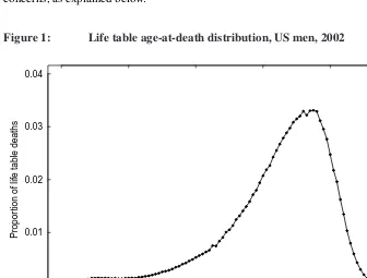
stand out (see Figure 1). Instead, there are several age candidates, a few years apart from each other, which leads to modal ages at death estimates that are also a few years apart from each other. This then translates into substantial artificial fluctuations in the estimated modal age at death trend over time. Note that Cheung, Robine, and Caselli (2008) fitted their quadratic models based on the[M∗−5, M∗+ 5]life table age range, raising other
concerns, as explained below.
Figure 1: Life table age-at-death distribution, US men, 2002
0.00 0.01 0.02 0.03 0.04
Age
Propor
tion of lif
e tab
le deaths
10 30 50 70 90 110
Cheung and Robine (2007) and Cheung et al. (2009) have instead been inspired by Lexis’s concept of normal life durations (Lexis 1877, 1878) to estimate the modal age at death. According to Lexis, if premature deaths are removed from all deaths, the “normal” deaths that remain are described by a normal distribution along age. Therefore, Cheung and her colleagues fitted a scaled normal model to life table deaths, starting five years before the age at which the highest number of deaths occurs in the life table. Although this procedure is appealing because it is theoretically oriented as proposed by Lexis, the scaled normal model imposes a strict “bell”-shaped structure to the selected life table deaths and any departure from this structure in the data is ignored. Furthermore, the age at which the fitting procedure starts first requires the identification of a single age with the highest number of deaths in the life table. As explained above, this can be problematic when there are several age candidates to choose from. Finally, systematically starting the fitting procedure five years before the age with the highest number of deaths in the life table to avoid including premature deaths in the modelling task is questionable. Indeed, the magnitude and the age profile of premature mortality have dramatically changed over the years and vary substantially across populations.
A simplified version of the logistic model of mortality, the Kannisto model of old-age mortality (Thatcher, Kannisto, and Vaupel 1998; Thatcher 1999), has also been exploited to estimate the modal age at death (Thatcher et al. 2010). However, this study by Thatcher et al. (2010) was oriented toward understanding the dynamics behind changes in the modal age at death over time rather than monitoring these changes closely. Using empirical death rates at ages 70 and 90 only to fit this simple logistic model, the authors found that the resulting modal age at death estimates were reasonably close to those computed with Kannisto’s (2001) quadratic method described above. Further theoretical considerations regarding the modal age at death and its related measures in several other mathematical models of mortality are provided by Canudas-Romo (2008) and Robine et al. (2006).
To our knowledge, Paccaud et al. (1998) were the only ones to rely on a nonpara-metric method to estimate the modal age at death. Nonparanonpara-metric models are seldom used for such a task, although they are generally more flexible than parametric models because they do not impose a predetermined structure on the observed data. In this paper, we demonstrate that the P-spline method provides the ability to refine the monitoring of changes in modal age at death over time.
2.2 Lifespan inequality
Mackenbach 1996). Based on period data from Sweden, Japan, and the USA, they found strong empirical correlation between these indicators. For ease of interpretation and com-putation, they recommended using the interquartile range to monitor changes in the vari-ability of age at death within human populations. Shortly after, Kannisto (2000) rather argued in favour of the C-family of indicators – i.e., the shortest age interval in which a given proportion of deaths occur – in particular because it allowed for a more com-plete analysis of mortality dispersion. He also suggested two other indicators to mea-sure variability in old age mortality instead of over the entire age range. One of them, a mode-based indicator called the standard deviation of ages at death above the mode, has been used in several subsequent studies on low mortality countries (Cheung, Robine, and Caselli 2008; Cheung et al. 2009; Cheung and Robine 2007; Kannisto 2001, 2007; Thatcher et al. 2010). As this measure of variability solely involves deaths occurring at ages above the mode, changes in the magnitude of premature mortality over time are less likely to influence the results.
In this paper, recent changes in the variability of adult mortality will be monitored with the standard deviation of ages at death above the mode. Specifically, this indicator corresponds to the root mean square of ages at death from the mode for individuals who lived up to or beyond the mode. A decline in this measure over time indicates that deaths above the mode have been compressed into a shorter age interval, hence the expressions
compression of deaths above the modeandold-age mortality compression. Given our objective to study recent adult mortality changes in low mortality countries, the fact that the standard deviation of ages at death above the mode directly measures variability in old-age mortality is an important asset.
Most variability indicators discussed in the literature have been computed with deaths extracted from life tables closed with a parametric model and/or involve the modal age at death, estimated using a parametric model. With the nonparametric smoothing approach based on P-splines, standard deviation of ages at death above the mode estimates are free from any kind of predetermined data structure with the potential to influence results.
2.3 Choice of a nonparametric method
When it comes to choosing a nonparametric modelling method to smooth data, there are several avenues. Under the running statistics category, there are notably kernel smoothers (Silverman 1986; Härdle 1990) and LOWESS – i.e., locally weighted scatterplot smoo-thing (Cleveland 1979). Then, spline methods are plentiful: for example, there are smoothing splines, regression splines (Eubank 1988), B-splines (de Boor 1978), and P-splines (Eilers and Marx 1996).
methods listed above, P-splines corresponds to the smoother that features most of these good properties simultaneously (see the Rejoinder section in Eilers and Marx (1996)). Of particular interest here, P-splines have no boundary effects and thus do not behave poorly near endpoints of the domain over which smoothing is performed (e.g., old ages in the context of mortality data). Also, P-splines have no trouble with sparse designs and there-fore work well even in cases where the domain includes gaps (e.g., ages at which zero deaths occur). The fact that the computed fit obtained with P-splines is described in a compact manner (see equation (1) in the next section) is also an important advantage over many of other smoothers available. Furthermore, P-splines are easy to use, program, and understand, while this is not necessarily the case for other nonparametric approaches. Fi-nally, previous studies have already demonstrated that P-splines are well-suited to the task of smoothing anomalously distributed data such as mortality data, given their grounding in generalized linear models (Currie, Durban, and Eilers 2004; Camarda 2008).
In this paper, the P-splines smoothing procedure will be applied to mortality data from age 10 and onwards. Infant and child mortality are excluded because they present unique features that would require the use of a smoothing method suited for ill-posed data; this goes well beyond the scope of the present study. Why not restrict the fitting procedure to the surroundings of the modal age at death? Starting at age 10 avoids the selection of another age interval, perhaps more subjectively, over which the smoothing procedure should take place. As discussed in section 2.1, the usual roughness in the mode area makes it difficult to identify a single age with the highest number of life table deaths. Restricting the fit to the surroundings of the mode would also involve choosing the length of the age interval over which the fitting procedure should take place. Whether this length should vary over time and across populations would also have to be debated. Another argument in favour of applying the fitting procedure from age 10 and onwards is that the analysis can then rely on a single smoothing method instead of several. Indeed, modal age at death estimates and standard deviation of ages at death above the mode estimates can all be computed based on the P-spline method.
3. Data and methods
onwards were selected. All years available on the HMD were used for Canada (1921– 2007) and Japan (1947–2009).
Letmi = di/ei denote the central death rate at agei for a given country, calendar year, and sex. Also, letµibe the force of mortality (or instantaneous death rate) at agei, such thatmi'µi+1
2 (Thatcher, Kannisto, and Vaupel 1998, Appendix A). Assuming that
the force of mortality is a piecewise constant function within each age and time interval – i.e.,µ(x) =µifor allx∈[i, i+ 1)– death countsdiare thus a realization of a Poisson distribution with meanei·µi(Alho and Spencer 2005, Chapter 4). Thispiecewise constant assumption in fact serves as a basis for computing empirical central death ratesmidefined above (Camarda 2008, p.4).
The Poisson regression model used in this paper also relies on this assumption. Fol-lowing the work of Eilers and Marx (1996), Currie, Durban, and Eilers (2004), and Ca-marda (2008), we used a flexible nonparametric approach based on B-splines with penal-ties known as P-splines to estimate the parameters of this model – i.e., the coefficients of the B-splines. The P-spline method is described in more detail in the Appendix, sections 1 to 3.
Smoothed forces of mortality are therefore computed according to
ˆ
µ(x) =exp(B(x)ˆa), (1)
whereBis the B-spline basis matrix andaˆis the vector of estimated coefficients for each B-spline included inB.
The corresponding smoothed survival function expressed as
ˆ
S(x) =exp
µ −
Z x
0 ˆ
µ(t)dt
can then be calculated using standard numerical integration techniques. Finally, the smoothed probability density function describing the age-at-death distribution for a given country, calendar year, and sex corresponds to
ˆ
f(x) = ˆµ(x) ˆS(x). (2)
We monitored changes in the various smoothed age-at-death distributions over time with their respective estimated modal age at death
ˆ
M = max
and estimated standard deviation of ages at death above the mode
\
SD(M+) =
v u u u u u t
Z ω
ˆ M
(x−Mˆ)2fˆ(x)dx
Z ω
ˆ M
ˆ
f(x)dx
,
whereωis the highest age attained in the population.
Note that the three curvesµ(x),S(x), andf(x)are related in such way that changes in one of them will necessarily be reflected in the others (Wilmoth 1997). In this paper, we mainly focus onfˆ(x), but analysis based onµˆ(x)or Sˆ(x) would yield consistent conclusions.
4. Results
This section is divided into two parts. First, an illustration of the nonparametric Poisson P-spline smoothing approach using Japanese data is provided. An analysis of recent trends in adult mortality in Canada, France, Japan, and the USA follows.
4.1 Illustration of the nonparametric P-spline approach using Japanese data
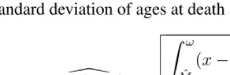
Figure 2 shows observed and fitted death counts in Japan by sex for a sample of years be-tween 1947 and 2008. We see that the Poisson regression models estimated with P-splines fit the data accurately. Indeed, the adjustedR2-measures based on deviance residuals for these fitted models (Mittlböck and Waldhör 2000) range from 0.9970 to 0.9998.
Figure 2: Comparison between observed death counts (points) and fitted death counts (lines) resulting from nonparametric P-spline estimations of Poisson regression models, Japan, selected years between 1947 and 2009
0.00 0.01 0.02 0.03 0.04
Age
Propor
tion of deaths
10 30 50 70 90 110
Women
1947 1965 1980 1995 2009
0.00 0.01 0.02 0.03 0.04
Age
Propor
tion of deaths
10 30 50 70 90 110
Men
1947 1965 1980 1995 2009
Figure 3: Smoothed density functions describing the age-at-death distribu-tion (standardized with respect to exposure to risk) and resulting from nonparametric P-spline estimations of Poisson regression models, Japan, selected years between 1947 and 2009
0.00 0.01 0.02 0.03 0.04 0.05
Age x
f
^ (x)
10 30 50 70 90 110
Women
1947 1965 1980 1995 2009
0.00 0.01 0.02 0.03 0.04 0.05
Age x
f
^ (x)
10 30 50 70 90 110
Men
1947 1965 1980 1995 2009
Figure 3 indicates that a great increase in the typical length of life occurred in Japan for both women and men during the 1950-2008 period, and that it was paralleled by a substantial decrease in lifespan inequality, at least until 1980. Indeed, as time went by, the age-at-death distributions have progressively moved to higher ages and became less and less spread out. However, accurate diagnosis are difficult with such visual inspection and simultaneous comparisons with other countries quickly become confusing. Time trends of summary measures such asMˆ andSD\(M+)are more informative, as shown in the next section.
4.2 Adult mortality trends in four low mortality countries
4.2.1 Modal age at death estimates (Mˆ)
Figure 4 presents sex-specific changes in average lifespan measured byMˆ in each of the four countries under study. It reveals thatMˆ increased substantially during the periods studied, although the increasing pace varied over time as well as across countries and sexes. Indeed, during the 1950s, 1960s, and 1970s, Japanese women were consistently showing the lowest modal age at death values, but their quick and steady mortality im-provements eventually led them well above the others. Thanks to an average growth rate of more than 3.3 months per year between 1947 and 2000,Mˆ reached 90 years in 2000. Such achievement in the level of the modal age at death occurred six years later among French women and has yet to be observed in Canada and the USA. However, after five decades of sustained increase inMˆ among Japanese women, the pace of increase slowed down and results for the most recent years even revealed an unexpected levelling off. In-deed, between 2004 and 2008, their modal age at death remained almost constant at about 91.0 years. In 2009, it reached 91.4 years.
Upward linear trends for Mˆ among French, Canadian, and US women have been recorded throughout most of the years studied, including the latest ones. Although the pace at whichMˆ increased since the mid-1940s for these women has been less spectacular than for the Japanese – i.e., 2.1 months per year on the average for French, 1.8 for Cana-dians, and 2.2 for Americans –Mˆ still reached 90.2 years in France in 2009, 89.2 years in Canada in 2007, and 88.7 years in USA in 2007. Interestingly, Canadian women have enjoyed a long-lasting advantage over the French with respect toMˆ, but since the begin-ning of the 1990s, this trend has been reversed. Similarly, US women recorded higher
ˆ
Figure 4: Estimated modal age at death based on smoothed density functions: Canada (1921–2007), France (1920–2009), Japan (1947–2009), and USA (1945–2007)
70 75 80 85 90
Year
M
^
1920 1930 1940 1950 1960 1970 1980 1990 2000 2010
Women
Canada France Japan USA
70 75 80 85 90
Year
M
^
1920 1930 1940 1950 1960 1970 1980 1990 2000 2010
Men
Canada France Japan USA
If we focus on results for men displayed in the bottom panel of Figure 4, we see that the rapid linear progression of the modal age at death in Japan also stands out. The average rate of increase forMˆ between 1947 and 2001 among Japanese men was above 2.9 months per year. However, a substantial slowdown occurred afterwards and their modal age at death only increased from 85.1 years in 2001 to 85.6 in 2009.
Since the beginning of the 1990s, French and Japanese men have been following each other very closely. Canadian men have also recently joined them, even though steady increases inMˆ only started in the early 1970s. As a matter of fact, from the 1920s to the 1960s, the modal age at death for Canadian men oscillated around 77 years, most probably because mortality reductions at ages older thanMˆ essential for its increase were limited during those years (Canudas-Romo 2010). Nevertheless, in 2006, the modal ages at death for men in Canada, Japan, and France were almost identical – i.e., about 85.7 years. Recall that disparities between these countries at that point in time were much greater among women. According to the latest results for 2009,Mˆ was slightly higher for French men (86.4 years) than it was for Japanese (85.6 years), but this might only be temporary.
In the USA, the upward trend forMˆ has been interrupted twice during the period un-der study:Mˆ decreased between 1962 and 1974, and between 2004 and 2006. The latter period reveals the most unforeseen decrease among US men. Indeed, at the beginning of the 1980s, US men caught up with Canadian men and their respective increasing trends inMˆ remained very similar for more than two decades afterwards, until the decrease oc-curred. Fortunately, the US modal age at death increased from 83.5 to 84.4 years between 2006 and 2007. Compared to the other three countries, US men are still lagging behind in 2007, but their delay is shorter than it was a few years ago.
4.2.2 Standard deviation of ages at death above the mode estimates (SD\(M+))
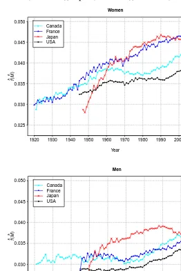
Figure 5: Estimated standard deviation of ages at death above the mode based on smoothed density functions: Canada (1921–2007), France (1920–2009), Japan (1947–2009), and USA (1945–2007)
5 6 7 8 9 10 11
Year
S
D
^
(M
+)
1920 1930 1940 1950 1960 1970 1980 1990 2000 2010
Women
Canada France Japan USA
5 6 7 8 9 10 11
Year
S
D
^(M
+)
1920 1930 1940 1950 1960 1970 1980 1990 2000 2010
Men
Canada France Japan USA
French and Canadian women reveal similar declining trends inSD\(M+)over time, although the level of old-age mortality disparity was almost always higher among the lat-ter. Between 1920 and 1960,SD\(M+)went from 7.8 to 6.8 years in France; in Canada, it went from 8.6 years in 1921 to 7.3 years in 1960. Recall that Japanese women accom-plished an equivalent reduction in their level of variability of age at death above the mode in one third of the time. After 1960, both French and Canadian women recorded a pause in decline forSD\(M+), but the decline resumed earlier in France than in Canada. Nonethe-less, since the early 2000s,SD\(M+)has been stagnating at about 6.3 years among Cana-dian women. Old-age mortality compression might have stopped as well among French women lately becauseSD\(M+)remained between 5.8 and 5.9 years since 2001, except in 2003 where it reached 5.7 years.
In the USA,SD\(M+)decreased very rapidly among women between 1945 and the early 1960s. Indeed, it went from 9.3 to about 7.2 years during that period. Afterwards, changes in variability of age at death above the mode ceased for two decades. Further decline inSD\(M+)was then observed between the early 1980s and late 1990s. In 2000,
\
SD(M+) reached 6.4 years among US women, and remained essentially unchanged from this time forward, signifying that old-age mortality compression has either been very weak lately or reached an end among these women. Still, for the most recent years studied, US women displayed the highestSD\(M+)results, while French women had the lowest ones.
From the men’s perspective, country-specific trends forSD\(M+) presented in the bottom panel of Figure 5 indicate that old-age mortality compression was strong in Japan from the 1950s to the early 1960s. Indeed,SD\(M+)went from about 9.5 to 7.5 years during that period. It declined at a much slower pace afterwards and reached 7.1 years in 1990. Since then, little change inSD\(M+)has been recorded among Japanese men, suggesting that their old-age mortality compression is essentially over.
Among French and Canadian men, the onset of decline inSD\(M+)occurred in the 1970s and roughly coincides with the onset of increase inMˆ (see section 4.2.1). Prior to the 1970s,SD\(M+)rather oscillated around a value of about 7.8 years in France and tended to increase at a very slow pace in Canada – i.e., from about 8.1 to 9.0 years in five decades. From the 1970s to 2000,SD\(M+)decreased consistently in both countries and finally reached 6.7 and 7.3 years among French and Canadian men respectively. Since then, SD\(M+) seems to be declining at a lesser pace than before, especially among Canadian men, but further decline in the level of variability of age at death above the mode is expected in upcoming years on this basis.
mid-1960s. Then, up to the mid-1970s, SD\(M+) increased and peaked at 10.1 years in 1974. Between the mid-1970s and the early 2000s,SD\(M+)followed a steep declining trend, which ended at 6.8 years in 2002. For four consecutive years afterwards,SD\(M+) increased drastically and reached 7.7 years in 2006. In 2007, it attained 7.4 years. Note that periods during which SD\(M+) stagnated among US men correspond to periods whereMˆ stagnated as well (see section 4.2.1). Furthermore, in periods whereSD\(M+) was increasing,Mˆ was decreasing and vice-versa. In particular, the unexpected upward trend inSD\(M+)recorded among US men in the latest years studied coincides with the sudden decrease inMˆ experienced between 2004 and 2006. Thus, despite the fact that at the turn of the twenty-first century, country-specific trends inSD\(M+)among men converged to a level close to 7 years, disparities grew larger afterwards. Based on the latest results, US men now display the highest values forSD\(M+)and are respectively followed by Japanese, Canadian, and French men.
5. Discussion
Transformations in the survival curve or in the age-at-death distribution over time have usually been monitored with indicators tied to various parametric statistical modelling techniques (e.g., quadratic model, normal model, or logistic model). In this paper, we in-troduced a nonparametric approach based on P-splines to refine the monitoring of changes in the central tendency and variability of adult lifespan over time. We believe that the P-spline method comes near to being the ideal way to estimate the modal age at death and its associated measures of variability of deaths. Indeed, in comparison with other alternative methods currently used, it has the following three key advantages. First, it is free from strong parametric assumptions about the shape of the distribution of deaths, otherwise susceptible to influence results. Second, it does not depend on an identified single age, which often does not clearly stand out, at which the highest number of deaths occurs in a life table. Finally, it avoids having to choose, perhaps subjectively, the age range over which the modelling procedure should take place. In sum, the P-spline method leads to detailed yet smoothed age-at-death distributions, as described by observed death counts and exposure to risk data. Modal age at death (M) and standard deviation of ages at death above the mode (SD(M+)) estimates computed from these smoothed age-at-death distributions provide precise monitoring of changes in adult mortality over time.
according to Kannisto’s quadratic procedure (Kannisto 2001). Compared to the trends shown in the bottom panel of Figure 4, trends inMˆ in Figure 6 are clearly less steady and often difficult to read. Likewise, trends inSD\(M+)in Figure 6 show much larger fluctu-ations compared to those displayed in the bottom panel of Figure 5, making interpretation hazardous.
In recent studies (Canudas-Romo 2008; Cheung, Robine, and Caselli 2008; Cheung and Robine 2007; Thatcher et al. 2010), authors have argued that the general scenario of compression of mortality, where increases in typical length of life are paralleled with decreases in variability of age at death, no longer describes appropriately recent adult mortality changes recorded in some low mortality countries. Instead, the shifting mor-tality regime (Bongaarts 2005; Kannisto 1996), where the log-force of mormor-tality among adults is assumed to shift downward and reach lower levels while keeping an intact shape, provides a better description. Under the shifting mortality regime, the age-at-death dis-tribution among adults thus shifts towards higher ages over time while retaining the same shape.
To investigate this further, we applied the P-spline method to a subset of four low mortality countries, namely Canada, France, Japan, and the USA. The results show that since the early 1990s, compression of deaths above the mode among Japanese women and men has stopped, while the mode continued to increase rapidly, at least until the early 2000s. In other words, Japan has been involved in the shifting mortality regime for several years now because its adult age-at-death distribution has been sliding to higher ages while retaining the same shape. These findings are thus consistent with those of the recent studies listed above. In particular, Cheung, Robine, and Caselli (2008), Cheung and Robine (2007), and Thatcher et al. (2010) also relied onSD(M+)to measure variability of adult lifespan and found that it levelled off or changed only slightly in Japan since the 1990s, whileM continued to increase.
Figure 6: Estimated modal age at death and standard deviation of ages at death above the mode among men based on Kannisto’s quadratic procedure: Canada (1921–2007), France (1920–2009), Japan (1947–2009), and USA (1945–2007)
70 75 80 85 90
Year
M
^
1920 1930 1940 1950 1960 1970 1980 1990 2000 2010
Estimated modal age at death
Canada France Japan USA
5 6 7 8 9 10 11
Year
S
D
^(M
+)
1920 1930 1940 1950 1960 1970 1980 1990 2000 2010
Estimated standard deviation above the mode
Canada France Japan USA
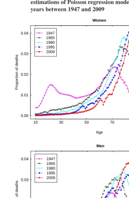
More evidence towards the shifting mortality regime was found among Canadian, US, and French women recently, but their male counterparts are still involved in the com-pression of mortality scenario. Of all four countries studied, the USA revealed the least favourable picture for the latest years, systematically recording the lowest modal age at death values. During the 2004-2006 period, US men even experienced a brief decline in their modal age at death. Our analysis also reveals that women and men in the USA often exhibited higher levels of variability of age at death above the mode compared to the other countries, including in very recent years. This US lifespan inequality disadvantage with respect to France, Japan and, to a lesser extent, Canada, is in fact even greater when dis-parities across a broader age range are considered. For example, Figure 7 displays time trends inf(M), the proportion of deaths occurring at the modal age at death. In other words,f(M)measures the level of concentration of individual life durations around the modal age at death (Kannisto 2001). More precisely,f(M)is the product ofS(M), the proportion of individuals living up to the mode or longer, byµ(M), the force of mortality at the mode. Thus,f(M)is much influenced by levels of infant and premature mortality, unlikeSD(M+)which essentially focuses solely on senescent mortality. Figure 7 shows that the US trend forf(M)has consistently been well below the others over the last five decades.
These findings regarding the USA are in line with those of Canudas-Romo (2008). Indeed, among the six industrialized countries studied by the author, including Japan and France, the USA displayed the lowest modal age at death estimates (sexes combined) since the mid-1980s, the highestSD(M+)estimates since the mid-1970s, and the lowest
f(M) estimates since the mid-1950s. The explanation for these results is not simple, but the large body of literature documenting socioeconomic inequalities prevailing in the USA and major differentials with respect to health plan coverage, health care access, and health care utilization (Murray et al. 2006) must account for some part of it. Analysing changes in the age-at-death distribution by socioeconomic subgroup could thus improve our current understanding of mortality dynamics among adults in the USA.
Figure 7: Estimated proportion of deaths occurring at the mode based on smoothed density functions: Canada (1921–2007), France (1920–2009), Japan (1947–2009), and USA (1945–2007)
0.025 0.030 0.035 0.040 0.045 0.050
Year
f
^ (M ^)
1920 1930 1940 1950 1960 1970 1980 1990 2000 2010
Women
Canada France Japan USA
0.025 0.030 0.035 0.040 0.045 0.050
Year
f
^ (M ^)
1920 1930 1940 1950 1960 1970 1980 1990 2000 2010
Men
Canada France Japan USA
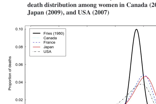
In conclusion, when Fries (1980) presented his theory on compression of mortality, he predicted that premature mortality would eventually be eliminated and that deaths would then follow a normal distribution with an average (modal) age at death of 85 years and a standard deviation of 4 years. Thirty years later, Robine and Cheung (2009) pointed out that the current picture actually looks very different (see Figure 8). Indeed, the modal age at death lies well above 85 years in several low mortality countries, at least among women, and their age-at-death distributions show much greater levels of variability of age at death. It seems very unlikely that human populations will ever reach the low level of variability hypothesized by Fries. Furthermore, contrary to what Fries had foreseen, the end of the general scenario of compression of mortality is not an end in itself. The shif-ting mortality regime has indeed received support following analysis of a growing number of low mortality countries lately. Nonetheless, whether on-going increases in longevity in these low mortality countries are paralleled with postponed diseases, functional limita-tions, and disability remains an open question. Mixed findings from recent studies (Chris-tensen et al. 2009; Robine, Saito, and Jagger 2009) decidedly calls for further research on the relationship between longevity and health.
Figure 8: Comparison between Fries’s predicted age-at-death distribution and the latest smoothed density functions describing the age-at-death distribution among women in Canada (2007), France (2009), Japan (2009), and USA (2007)
0.00 0.02 0.04 0.06 0.08 0.10
Age
Propor
tion of deaths
10 30 50 70 90 110
Fries (1980) Canada France Japan USA
6. Acknowledgements
References
Alho, J.M. and Spencer, B.D. (2005).Statistical demography and forecasting. New York: Springer.
Bongaarts, J. (2005). Long range trends in adult mortality: Models and projection methods.Demography42(1): 23–49.doi:10.1353/dem.2005.0003.
Brown, D.C., Hayward, M.D., Montez, J.K., Hummer, R.A., Chiu, C., and Hidajat, M.M. (forthcoming). The significance of education for mortality compression in the United States.Demography.
Camarda, C.G. (2008). Smoothing methods for the analysis of mortality development. [PhD Thesis]. Madrid: Universidad Carlos III de Madrid, Department of Statistics. Canudas-Romo, V. (2008). The modal age at death and the shifting mortality hypothesis.
Demographic Research19(30): 1179–1204.doi:10.4054/DemRes.2008.19.30. Canudas-Romo, V. (2010). Three measures of longevity: Time trends and record values
for longevity.Demography47(2): 299–312. doi:10.1353/dem.0.0098.
Cheung, S.L.K. and Robine, J. (2007). Increase in common longevity and the com-pression of mortality: The case of Japan. Population Studies 61(1): 85–97. doi:10.1080/00324720601103833.
Cheung, S.L.K., Robine, J.M., and Caselli, G. (2008). The use of cohort and period data to explore changes in adult longevity in low mortality countries. GenusLXIV(1-2): 101–129.
Cheung, S.L.K., Robine, J., Paccaud, F., and Marazzi, A. (2009). Dissecting the compres-sion of mortality in Switzerland, 1876-2005.Demographic Research21(19): 569–598. doi:10.4054/DemRes.2009.21.19.
Cheung, S.L.K., Robine, J., Tu, E.J., and Caselli, G. (2005). Three dimensions of the sur-vival curve: Horizontalization, verticalization, and longevity extension. Demography
42(2): 243–258.doi:10.1353/dem.2005.0012.
Christensen, K., Doblhammer, G., Rau, R., and Vaupel, J.W. (2009). Ageing popula-tions: The challenges ahead. The Lancet374(9696): 1196–1208. doi:10.1016/S0140-6736(09)61460-4.
Cleveland, W.S. (1979). Robust locally weighted regression and smoothing scat-ter plots. Journal of the American Statistical Association 74(368): 829–836. doi:10.2307/2286407.
rates.Statistical Modelling4(4): 279–298.doi:10.1191/1471082X04st080oa. de Boor, C. (1978).A practical guide to splines. Berlin: Springer.
Eakin, T. and Witten, M. (1995). How square is the survival curve of a given species?
Experimental Gerontology30(1): 33–64.doi:10.1016/0531-5565(94)00042-2. Edwards, R.D. and Tuljapurkar, S. (2005). Inequality in life spans and a new perspective
on mortality convergence across industrialized countries.Population and Development Review31(4): 645–674. doi:10.1111/j.1728-4457.2005.00092.x.
Eilers, P.H.C. and Marx, B.D. (1996). Flexible smoothing withB-splines and penalties (with discussion). Statistical Science11(2): 89–121.doi:10.1214/ss/1038425655. Eubank, R.L. (1988). Spline smoothing and nonparametric regression. New York:
Dekker.
Fries, J.F. (1980). Aging, natural death, and the compression of morbidity. New England Journal of Medicine303: 130–135.doi:10.1056/NEJM198007173030304.
Härdle, W. (1990).Applied nonparametric regression. Cambridge: Cambridge University Press.
Hill, G. (1993). The entropy of the survival curve: An alternative measure. Canadian Studies in Population20(1): 43–57.
Horiuchi, S. (2003). Interspecies differences in the life span distribution: Human versus invertebrates. In: Carey, J. R. and Tuljapurkar, S. (eds.). Population and Development Review29(Supplement): 127–151.
Human Mortality Database (2011). University of California, Berkley (USA), and Max Planck Institute for Demographic Research (Germany). Available at http://www.mortality.org or http://www.humanmortality.de (data downloaded on 6/8/2011).
Kannisto, V. (1996). The advancing frontier of survival life tables for old age. Odense: Odense University Press (Monographs on Population Aging 3).
Kannisto, V. (2000). Measuring the compression of mortality. Demographic Research
3(6).doi:10.4054/DemRes.2000.3.6.
Kannisto, V. (2001). Mode and dispersion of the length of life. Population: An English Selection13(1): 159–171.
Nether-lands: Springer: 111–129.doi:10.1007/978-1-4020-4848-7_5.
Keyfitz, N. (1977).Applied mathematical demography. New York: John Wiley and Sons. Lexis, W. (1877). Zur Theory der Massenerscheinungen in der menschlichen
Gesellschaft. Freiburg i.B.: Fr. Wagner’sche Buchhandlung.
Lexis, W. (1878). Sur la durée normale de la vie humaine et sur la théorie de la stabilité des rapports statistiques.Annales de Démographie Internationale2: 447–460. Lynch, S.M. and Brown, J.S. (2001). Reconsidering mortality compression and
de-celeration: An alternative model of mortality rates. Demography 38(1): 79–95. doi:10.1353/dem.2001.0007.
Manton, K.G. and Tolley, H.D. (1991). Rectangularization of the survival curve.Journal of Aging and Health3(2): 172–193.doi:10.1177/089826439100300204.
Martel, S. and Bourbeau, R. (2003). Compression de la mortalité et rectangularisation de la courbe de survie au Québec au cours du XXesiècle.Cahiers québécois de
démogra-phie32(1): 43–75.
Mittlböck, M. and Waldhör, T. (2000). Adjustments for R2-measures for Poisson regression models. Computational Statistics and Data Analysis 34(4): 461–472. doi:10.1016/S0167-9473(99)00113-9.
Murray, C.J., Kulkarni, S.C., Michaud, C., Tomijima, N., Bulzacchelli, M.T., Iandiorio, T.J., and Ezzati, M. (2006). Eight Americas: Investigating mortality disparities across races, counties, and race-counties in the United States. PLoS Medicine3(9): 1513– 1524.doi:10.1371/journal.pmed.0030260.
Myers, G.C. and Manton, K.G. (1984a). Compression of mortality: Myth or reality? The Gerontologist24(4): 346–353.doi:10.1093/geront/24.4.346.
Myers, G.C. and Manton, K.G. (1984b). Recent changes in the U.S. age at death distribution: Further observations. The Gerontologist 24(6): 572–575. doi:10.1093/geront/24.6.572.
Nagnur, D. (1986). Rectangularization of the survival curve and entropy: The Canadian experience, 1921-1981.Canadian Studies in Population13(1): 83–102.
Nelder, J.A. and Wedderburn, R.W.M. (1972). Generalized linear models. Journal of the Royal Statistical Society. Series A135(3): 370–384.doi:10.2307/2344614.
Nusselder, W.J. and Mackenbach, J.P. (1997). Rectangularization of the survival curve in the Netherlands: An analysis of underlying causes of death. Journal of Gerontology: Social Sciences52B(3): S145–S154.doi:10.1093/geronb/52B.3.S145.
O’Sullivan, F. (1988). A statistical perspective on ill-posed inverse problems (with dis-cussion).Statistical Science1(4): 505–527.
Ouellette, N. (2011). Changements dans la répartition des décès selon l’âge : une ap-proche non paramétrique pour l’étude de la mortalité adulte. Montreal: Université de Montréal, Department of Demography. [PhD Thesis].
Paccaud, F., Pinto, C.S., Marazzi, A., and Mili, J. (1998). Age at death and rectangulariza-tion of the survival curve: Trends in Switzerland, 1969-1994.Journal of Epidemiology and Community Health52(7): 412–415. doi:10.1136/jech.52.7.412.
Pearson, K. (1902). On the modal value of an organ or character. Biometrika1(2): 260– 261. doi:10.2307/2331492.
Robine, J. (2001). Redéfinir les phases de la transition épidémiologique à travers l’étude de la dispersion des durées de vie: le cas de la France. Population56(1-2): 199–222. doi:10.2307/1534822.
Robine, J. and Cheung, S.L.K. (2009). Nouvelles observations sur la longévité humaine.
Revue Économique59(5): 941–953. doi:10.3917/reco.595.0941.
Robine, J., Cheung, S.L.K., Thatcher, A.R., and Horiuchi, S. (2006). What can be learnt by studying the adult modal age at death? Paper presented at the Annual Meeting of the Population Association of America, Los Angeles, California, March 30-April 1, 2006.
Robine, J., Saito, Y., and Jagger, C. (2009). The relationship between longevity and healthy life expectancy.Quality in Aging and Older Adults10(2): 5–14.
Rothenberg, R., Lentzner, H.R., and Parker, R.A. (1991). Population aging patterns: The expansion of mortality. Journal of Gerontology: Social Sciences46(2): S66–S70. doi:10.1093/geronj/46.2.S66.
Silverman, B.W. (1986). Density estimation for statistics and data analysis. London: Chapman and Hall.
Thatcher, A.R. (1999). The long-term pattern of adult mortality and the highest attained age.Journal of the Royal Statistical Society. Series A162(1): 5–43. doi:10.1111/1467-985X.00119.
com-pression of deaths above the mode. Demographic Research 22(17): 505–538. doi:10.4054/DemRes.2010.22.17.
Thatcher, A.R., Kannisto, V., and Vaupel, J.W. (1998). The force of mortality at ages 80 to 120. Odense: Odense University Press (Monographs on Population Aging 5). Wilmoth, J.R. (1997). In search of limits. In: Wachter, K.W. and Finch, C.E. (eds.)
Between Zeus and the salmon: The biodemography of longevity. Washington D.C.: National Academy Press: 38–63.
Appendix
In this appendix, we provide an introduction to P-splines, which are used in this paper to smooth mortality data. In a nutshell, the P-spline method is a nonparametric approach that combines the concepts of B-spline and penalized likelihood. B-splines provide flexibility, which leads to an accurate fit of the data, while the penalty, which acts on the coefficients of adjacent B-splines, ensures that the resulting fit behaves smoothly. Comparison be-tween HMD life table age-at-death distributions and P-spline smoothed density functions for Japan are presented in the last section of the appendix.
A1. From B-splines to P-splines
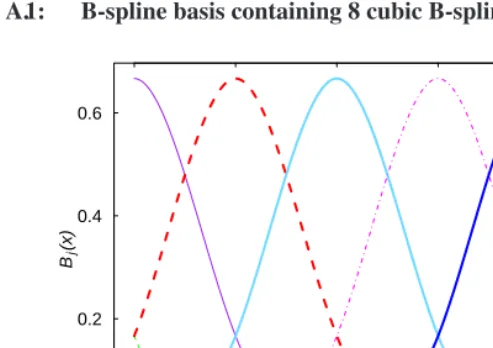
The termB-splineis short for basis spline, and, as splines in general, B-splines are made out of polynomial pieces that are joined together at points calledknots. The degree of the B-splines (e.g., degree 1: linear, degree 2: quadratic, degree 3: cubic, and so on) is set by the user and given by the degree of the polynomial pieces used to build them.
What makes B-splines attractive is that each B-spline is non-zero on a limited range of the interval over which the smoothing procedure is taking place. This also means that in any given point of the interval, only a few B-splines are non-zero, thus offering greatlocal
control in the resulting fit. Increasing the number of knots in the interval will increase the amount of B-splines and thus enhance the ability to capture variation in the data.
B-spline basis are well-suited for smoothing observed data points, say(xi, zi),i =
1, . . . , n. Figure A.1 shows an example of a B-spline basis, which includes 8 equally
spaced B-splines of degree 3, namely cubic B-splines. The basis matrixB associated with this B-spline basis is defined as
B=
B1(x1) B2(x1) . . . B8(x1)
B1(x2) B2(x2) . . . B8(x2)
..
. ... ... ...
B1(xn) B2(xn) . . . B8(xn)
,
whereBj(xi),j = 1, . . . ,8denotes the value atxi of thejth cubic B-spline. A fitted curvezˆto observed data points(xi, zi)is then expressed aszˆ(xi) =
P8
j=1aˆjBj(xi),
where(ˆa1,ˆa2, . . . ,ˆa8)> is the vector of estimated regression parameters. Each of these regression parameters is associated to one B-spline in the basis and determines its height. More generally, we have
ˆ
z=Baˆ, (A.1)
Figure A.1: B-spline basis containing 8 cubic B-splines with equally spaced knots
0.0 0.2 0.4 0.6 0.8 1.0 x
Bj
(x)
0.0 0.2 0.4 0.6
Source: Authors’ calculations.
The task of choosing the optimal number of knots and their position in the interval [minixi;maxixi]is a rather complex one. With the P-spline method, this task is avoided.
Indeed, inspired by the work of O’Sullivan (1988), Eilers and Marx (1996) developed P-splines by combining B-P-splines and difference penalties on the estimated coefficients of adjacent B-splines. The idea behind this approach is to use a relatively generous amount of equally spaced knots on the interval, and to apply a penalty on adjacent regression coefficients to ensure smooth behaviour and avoid over-fitting the data.
A2. The penalized likelihood function for P-splines
With the P-spline approach, the estimated vector of coefficientsaˆgiven in equation (A.1) results from a maximization of the following penalized log-likelihood function:
l∗=l(a;B;z)−1
2a
0P a. (A.2)
The role of the penalty term in equation (A.2) is illustrated on simulated data in Figure A.2. The left panel shows the results obtained when the penalty is omitted. In such cases, the fitted curve is very erratic because the estimated coefficients of adjacent B-splines are allowed to vary sharply from one another. Indeed, from the various B-splines shown at the bottom of the illustration, we note several sudden changes in their heights. The right panel of Figure A.2 shows a fitted curve that is much smoother because the penalty is taken into account and this forces the estimated coefficients of adjacent B-splines to vary smoothly. Thus, the height of neighbouring B-splines can no longer change abruptly.
Figure A.2: Unpenalized (left panel) and penalized (right panel) regression using simulated data and 23 equally spaced cubic B-splines
Source: Authors’ calculations.
A3. Smoothing mortality data with P-splines
Letd, e,µdenote respectively observed death counts, exposures to risk, and force of mortality vectors for a given country, calendar year, and sex. Since our response variable
dis assumed to be Poisson distributed, we introduce a linear predictorηsuch that
η=ln(E[d]).
Thus,ηcan be modelled by a linear combination of unknown parameters. As mentioned in section 3., the P-spline approach is used in this paper to estimate those parameters. More precisely, the model corresponds to
whereBis the B-spline basis matrix andais the vector of respective regression parame-ters to estimate. Furthermore, the logarithm of exposure to risk, ln(e), is commonly referred to as theoffsetin a Poisson regression setting.
Using the P-spline method adapted for Poisson death counts to estimatea, we obtain
ˆ
η=ln(e) +Baˆ. (A.3)
Taking the exponential of equation (A.3) gives smoothed death counts, which are however influenced by exposure to riskeand therefore not comparable from one age, sex, calendar year or country to another. In order to obtain comparable – i.e., standardized – age-at-death distributions, one must extract the smoothed forces of mortality from the smoothed death counts. Given equation (A.3), a smoothed trend for the force of mortality is readily obtained as
ˆ
µ(x) =exp(B(x)ˆa).
In the context of mortality data, the penalized log-likelihood function to maximize in order to findaˆinvolved in equation (A.3) specifically corresponds to
l∗=l(a;B;d)−1
2a 0P a
=l(a;B;d)−1
2λa
0D0Da. (A.4)
In the latter equation,l(a;B;d)is the usual log-likelihood function for a generalized linear model andP =λD0Dis the penalty matrix. For any given smoothing parameter λand difference matrix D, the maximization of equation (A.4) can be solved with a penalized version of the iteratively reweighted least squares algorithm for the estimation of generalized linear models (Nelder and Wedderburn 1972) (see also Currie, Durban, and Eilers (2004) and Camarda (2008) for further details).
In this paper, we used a second order – i.e., quadratic – difference matrixDsuch that
a0D0Da= (a
1−2a2+a3)2+ (a2−2a3+a4)2+. . ., and the smoothing parameter
λwas selected according to the Bayesian Information Criterion, as suggested by Currie, Durban, and Eilers (2004). Regarding the B-spline basis, we used cubic B-splines and one knot per every five data point on the age interval.
A4. Comparison between HMD life table age-at-death distributions and P-spline smoothed density functions for Japan
data were extracted from the HMD and the smoothed density functions were computed according to equation (2).
Figure A.3: Comparison between HMD life table age-at-death distributions (overplotted points and lines) and smoothed density functions (plain solid lines) resulting from nonparametric P-spline estima-tions of Poisson regression models, Japan, selected years between 1947 and 2009
0.00 0.01 0.02 0.03 0.04 0.05
Age
Propor
tion of deaths
10 30 50 70 90 110
Women
1947 1965 1980 1995 2009
0.00 0.01 0.02 0.03 0.04 0.05
Age
Propor
tion of deaths
10 30 50 70 90 110
Men
1947 1965 1980 1995 2009