The geospace response to variable inputs from the lower atmosphere: a review of the progress made by Task Group 4 of CAWSES-II

R E V I E W

Open Access

The geospace response to variable inputs from the

lower atmosphere: a review of the progress made

by Task Group 4 of CAWSES-II

Jens Oberheide

, Kazuo Shiokawa

, Subramanian Gurubaran

, William E Ward

, Hitoshi Fujiwara

,

Michael J Kosch

, Jonathan J Makela

and Hisao Takahashi

Abstract

The advent of new satellite missions, ground-based instrumentation networks, and the development of whole atmosphere models over the past decade resulted in a paradigm shift in understanding the variability of geospace, that is, the region of the atmosphere between the stratosphere and several thousand kilometers above ground where atmosphere-ionosphere-magnetosphere interactions occur. It has now been realized that conditions in geospace are linked strongly to terrestrial weather and climate below, contradicting previous textbook knowledge that the space weather of Earth's near space environment is driven by energy injections at high latitudes connected with magnetosphere-ionosphere coupling and solar radiation variation at extreme ultraviolet wavelengths alone. The primary mechanism through which energy and momentum are transferred from the lower atmosphere is through the generation, propagation, and dissipation of atmospheric waves over a wide range of spatial and temporal scales including electrodynamic coupling through dynamo processes and plasma bubble seeding. The main task of Task Group 4 of SCOSTEP's CAWSES-II program, 2009 to 2013, was to study the geospace response to waves generated by meteorological events, their interaction with the mean flow, and their impact on the ionosphere and their relation to competing thermospheric disturbances generated by energy inputs from above, such as auroral processes at high latitudes. This paper reviews the progress made during the CAWSES-II time period, emphasizing the role of gravity waves, planetary waves and tides, and their ionospheric impacts. Specific campaign contributions from Task Group 4 are highlighted, and future research directions are discussed.

Keywords:Geospace; Thermosphere; Ionosphere; Tides; Planetary waves; Gravity waves; Traveling ionospheric disturbances; Traveling atmospheric disturbances

Introduction

The space weather of Earth's upper neutral and ionized at-mosphere is strongly influenced by energy injections at high latitudes connected with magnetosphere-ionosphere coupling and solar radiation variability at extreme ultra-violet wavelengths. A variety of new evidence obtained over the past few years now demonstrates unequivocally that the geospace environment also owes a substantial amount of its variability to waves forced in the lower parts of Earth's atmosphere, that is, the troposphere and strato-sphere. This paradigm shift in understanding the causes of

geospace variability was made possible by the advent of satellite missions like Imager for Magnetopause-to-Aurora Global Exploration (IMAGE) (Burch 2000), Thermosphere Ionosphere Mesosphere Energetics and Dynamics (TIMED) (Yee et al. 1999), CHAllenging Minisatellite Payload (CHAMP) (Reigber et al. 2006), Gravity Recovery and Climate Experiment (GRACE) (Tapley et al. 2004), and Constellation Observing System for Meteorology (COSMIC) (Anthes et al. 2008), advanced ground-based observing cap-abilities like Poker Flat Advanced Modular Incoherent Scatter Radar (PFISR) (e.g., Nicolls and Heinselman 2007) and airglow observing networks (e.g., Shiokawa et al. 2009; Makela et al. 2009), and the development of ‘whole atmosphere’general circulation models from the ground to the ionosphere such as Whole Atmosphere Community

* Correspondence:[email protected] 1

Department of Physics and Astronomy, Clemson University, Clemson, SC 29634-0978, USA

Full list of author information is available at the end of the article

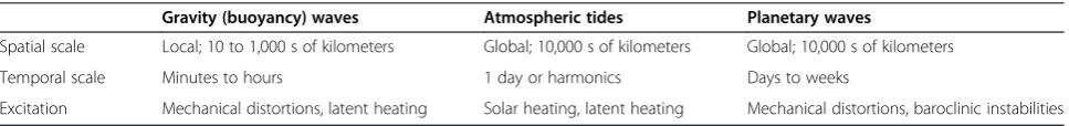
Climate Model - thermosphere extension (WACCM-X) (Liu et al. 2010a), Whole Atmosphere Model (WAM)/ Coupled Thermosphere Ionosphere Plasmasphere Electro-dynamics Model (CTIPe) (Fuller-Rowell et al. 2010), and ground-to-topside model of Atmosphere and Ionosphere for Aeronomy (GAIA) (Jin et al. 2011). See the list of ab-breviations at the end of the paper. It is by now without dispute that geospace owes much of its longitudinal, seasonal-latitudinal, and day-to-day variability to me-teorological weather processes in the troposphere and stratosphere (e.g., Immel et al. 2006; Forbes et al. 2006; Oberheide et al. 2006b; Hagan et al. 2007; Goncharenko et al. 2010; Fritts and Lund 2011; Maute et al. 2012; and references therein). The primary mechanism through which energy and momentum are transferred from the lower atmosphere is through the propagation and dis-sipation of atmospheric waves, including electrodynamic coupling through dynamo processes and instability seed-ing. Table 1 summarizes the basic characteristics of the three most important classes of atmospheric waves: grav-ity waves (GWs), atmospheric tides, and planetary waves (PWs).

CAWSES-II Task Group 4 (TG4; What is the geospace response to variable inputs from the lower atmosphere?) was therefore charged to elucidate the dynamical coupling from the low and middle atmosphere to the geospace (i.e., the upper atmosphere, ionosphere, and magneto-sphere), for various wave frequencies and scales, and for equatorial, middle, and high latitudes. As meeting the challenge clearly requires a systems approach in-volving experimentalists, data analysts, and modelers from different communities, an essential part of TG4 was to encourage interactions between atmospheric scientists and plasma scientists on all occasions. To distinguish geospace variability due to solar and mag-netospheric driving from above from processes propa-gating from below, and in order to dissect the problem into solvable pieces, four projects were formed to respect-ively address each of the following science questions: (1) How do atmospheric waves connect tropospheric weather with ionosphere/thermosphere variability? (2) What is the relation between atmospheric waves and ionospheric in-stabilities? (3) How do the different types of waves interact as they propagate through the stratosphere to the iono-sphere? (4) How do thermospheric disturbances generated by auroral processes interact with the neutral and ionized atmosphere?

Several observational campaigns were conducted within each project, supported by regular workshops, conference sessions, and business meetings. Results were not only dis-seminated through the peer-reviewed literature but also to the broader CAWSES community through quarterly TG4 newsletters. This paper describes these activities and re-views the progress made over the CAWSES-II period from 2009 to 2013. Each project and its scientific out-comes are described in a separate section. The manuscript concludes with a general discussion of the outcomes, the scientific challenges for the future, new satellite missions, and SCOSTEP's new VarSITI program. More results related to TG4 can be found in the four special issues listed in Table 2 and in a special issue of Earth, Planets and Space dedicated to results presented at the International CAWSES-II Symposium (2014) held at Nagoya University, Japan, 18 to 22 November 2013.

Review

Project 1: How do atmospheric waves connect tropospheric weather with ionosphere/thermosphere variability?

The impact of atmospheric waves on ionospheric structure and variability has been realized for quite some time. Hines (1960) in his pioneering work was the first to propose GW as the cause of‘irregular motions’in the thermosphere and ionosphere. Since then, numerous studies have revealed that GWs are present at heights up to the upper thermo-sphere and connected them to medium-scale traveling ionospheric disturbances (MSTIDs), ionospheric irregular-ities, and plasma instabilities. See for example the more re-cent review by Fritts and Lund (2011) and references therein. Before CAWSES-II, it was already known that GW from convection and jet streams in the lower atmos-phere propagate into the mesosatmos-phere, dissipate their en-ergy near the mesopause region, and/or penetrate into the thermosphere. However, despite some speculation about the initiation of various plasma instabilities by GW, the re-lation between GW and MSTID, day-to-day variability and zonal separation of plasma bubbles, and the scale size and propagation of sporadic-E patches were not understood. The examination of the relationship between these phe-nomena and an improved understanding of the importance of GW in ionosphere/thermosphere dynamics were objec-tives for CAWSES-II.

The idea that global winds in the ionosphere may be a source of disturbance electric fields and currents goes

Table 1 Basic characteristics of atmospheric waves

Gravity (buoyancy) waves Atmospheric tides Planetary waves

Spatial scale Local; 10 to 1,000 s of kilometers Global; 10,000 s of kilometers Global; 10,000 s of kilometers

Temporal scale Minutes to hours 1 day or harmonics Days to weeks

back at least to the dynamo theory by Stewart (1882); the connection to Sun-synchronous (migrating) atmos-pheric tides forced by solar radiation absorption was dis-cussed by Fejer (1964). As tidal theory and observational diagnostics progressed, it was realized that non Sun-synchronous (nonmigrating) tides forced by deep tropical convection are equally important for explaining longitu-dinal and local time variations in bulk neutral and plasma properties of the ionosphere/thermosphere system. Satel-lite diagnostics (Forbes et al. 2006; Oberheide et al. 2006b; Sagawa et al. 2005; Immel et al. 2006) and models (Hagan and Forbes 2002; Hagan et al. 2007) resulted in a basic quantitative knowledge of tidal forcing, propagation, and morphology in the mesosphere and lower thermosphere, the ionosphere, and a basic qualitative knowledge about the coupling into the F-region through E-region dynamo modulation. It should be noted that important contribu-tions came from CAWSES-I activities, for example, from the CAWSES tidal campaigns (Ward et al. 2010) that ef-fectively resolved the long-standing issue between ground-based radar and satellite optical measurements of winds. See also Kishore Kumar et al. (2013) for a recent compari-son between radar, satellite, and model results obtained during the first CAWSES tidal campaign in 2005. Major challenges for CAWSES-II included the elucidation of

tidal structures in the altitude range between 110 (upper altitude observed by TIMED) and 400 km (in situtidal diagnostics from CHAMP) where suitable satellite ob-servations are lacking, temporal variations of the tides on timescales ranging from days to solar cycle, a better separation of E-region dynamo modulation vs tidal coupling at F-region heights, an assessment of the tidal impacts on the energy balance and composition of the thermosphere, and wave-wave and wave-mean flow in-teractions. Similar questions are applied to PW as well, with special interest in their role in connecting polar stratospheric warmings with F-region low latitude plasma density variability (Goncharenko and Zhang 2008), as fur-ther detailed in project 3.

Gravity waves

Gravity waves generated by convective systems, hurri-canes, and surface perturbations such as earthquakes and tsunamis may seed plasma bubbles in the ionosphere through Rayleigh-Taylor instability. Figure 1 shows GW in airglow images at 630 nm (approximately 250 km) caused by the tsunami from the catastrophic Tohoku earthquake on 11 March 2011 when it passed the Hawaiian Islands. See Makela et al. (2011) for details and also for a movie that includes the ionospheric response in total electron Table 2 Special issues with significant TG4 contributions

Title Journal Year TG4 relation

Coupling between the lower and upper atmosphere JGR Space Physics 2010 General topic

Coupling between the Earth's atmosphere and its plasma environment

Space Science Review, Vol. 168, Issue 1-4, 2012

2012 ISSI workshop, see TG4 newsletter vol. 3

Recent progress in the vertical coupling in the atmosphere-ionosphere system

J. Atmos. Sol. Terr. Phys., Vol. 90-91, pages 1-222, December 2012

2012 4th IAGA/ICMA/CAWSES-II TG4 workshop on vertical coupling

Recent advances in equatorial, low-, and mid-latitude aeronomy

J. Atmos. Sol. Terr. Phys., Vol. 103, pages 1-194, October 2013

2013 ISEA-13 conference

content (TEC). The ionospheric response over Japan (Figure 2) for the same event shows very pronounced concentric waves in TEC that propagate in the radial direction with a velocity between 138 and 3,457 m/s with an‘ionospheric epicenter’about 170 km southeast from the earthquake epicenter (Tsugawa et al. 2011). The initial signatures in Figure 2 with a propagation velocity of 3,457 m/s are most likely caused by a Rayleigh wave (a type of surface wave during earthquakes), followed by acoustic waves triggered by the Rayleigh wave. Finally, medium-scale concentric waves with a propagation vel-ocity of 138 to 423 m/s were detected 300 km away from the ionospheric epicenter (Figure 2g,h). They are the result of GW forced by the surface displacement (Matsumura et al. 2011).

Nishioka et al. (2013) discussed similar concentric waves in the ionospheric TEC variation over the North-American continent as an indicator of thermospheric gravity waves generated by the 2013 Moore EF5 tornado. Fukushima et al. (2012) showed correlation of MSTIDs observed by a 630 nm airglow imager over Indonesia with tropospheric convective activity but with the average horizontal wave-length of the MSTIDs increasing with decreasing solar ac-tivity. These findings suggest that the observed MSTIDs in the equator are caused by secondary gravity waves in the thermosphere, possibly generated by tropospheric convect-ive activity. Smith et al. (2013) reported on thermospheric secondary GWs generated from mountain wave breaking

in the upper mesosphere using a simultaneous observation of 630 nm and 557.7 nm airglow images over New Zealand.

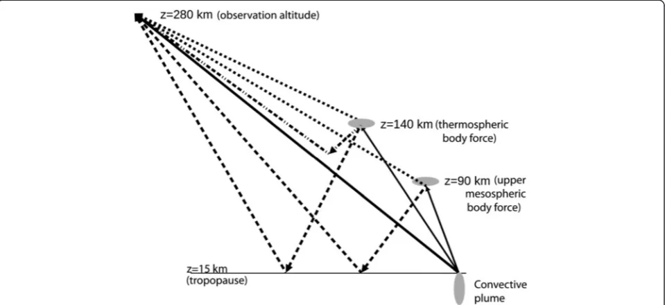
Progress in gravity wave theory (e.g., Vadas and Liu 2009; Vadas and Crowley 2010; Yiğit et al. 2012; Gavrilov and Kshetvetskii 2014) now provides a much clearer pic-ture of how gravity waves from the lower atmosphere can reach thermospheric altitudes, involving a multitude of possible pathways including direct propagation, reflection in the upper atmosphere, and the generation of secondary waves through upper mesospheric and thermospheric body forces (Figure 3). As a result, substantial neutral horizontal wind and plasma density variations from a single convective plume are predicted to occur as far away as adjacent continents, pointing to local wave sources having a global impact: a significant challenge for the interpretation of observations. An example of the ionospheric response to convective activity over Brazil on 1 October 2005 is shown in Figure 4 which is adapted from Vadas and Liu (2013). Thermospheric body forces resulting from convective plumes are com-puted with the Vadas model. Their incorporation into the Thermosphere-Ionosphere-Mesosphere-Electrodynamics General Circulation Model (TIME-GCM) results in large-scale traveling ionospheric disturbances. Of note is that the hmF2′perturbations are generally anticorrelated with the foF2′ and TEC′ perturbations. This indicates that field-aligned transport instead of chemistry (i.e., [e ] + [O+] recombination) may be the dominant coupling

mechanism into the plasma. Observing such signa-tures still poses a significant challenge. Corresponding temperature perturbations in the thermosphere (not shown) will be observed from geostationary orbit in the near future by the Global-scale Observations of the Limb and Disk (GOLD) instrument (a UV imager to be launched in 2017; Eastes et al. 2008). For the ionospheric signatures, much progress can be ex-pected from Swarm, an ESA constellation mission (Haagmans et al. 2013) that was launched in 2013. The role of GW for ionospheric instability seeding was the focus of TG4 project 2 and is further discussed in the corresponding section later in this paper.

Tides

The components of the tidal spectrum that follow the apparent westward propagation of the Sun relative to the Earth's surface are called migrating tides, and the non-Sun-synchronous components are called nonmi-grating tides. Minonmi-grating tides are predominantly forced by solar radiation absorption in tropospheric water vapor and stratospheric ozone. Nonmigrating tides are thought to have two major sources: non-linear wave-wave inter-action processes in the strato-/mesosphere (Hagan and Roble 2001) and latent heating due to large-scale deep convection in the tropical troposphere (Hagan and Forbes 2002, 2003). Deep convection largely depends on land-sea differences and sea-surface temperatures. Variations in the periodic absorption of solar radiation at the surface thus transform to a longitudinal structure in raindrop forma-tion (heat release) at roughly the same local time of the

day that acts as an efficient forcing mechanism for a num-ber of nonmigrating tides including the diurnal eastward propagating tide of zonal wavenumber 3 (DE3). Note that the DE3 appears as a zonal wavenumber 4 (wave-4) longi-tudinal structure when observed at constant local solar time, e.g., by precessing satellites in a low Earth orbit. This is simply a result of its eastward propagation and frequency.

Figure 5 summarizes the pre-CAWSES-II knowledge of the cause-and-effect chain between latent heat forcing, tidal propagation, and coupling into the ionosphere, based on various satellite observations. The most striking pat-tern is a 4-peaked‘wave-4’longitudinal modulation that is apparent in deep convective cloud occurrence, E-region zonal winds, thermospheric constituents, F-region elec-tron and ion density, and upper thermosphere neutral mass density. Nonmigrating tidal winds in the low and middle latitude E-region move the partially ionized plasma through Earth's magnetic field while the electrons with their high gyro frequency/collision frequency ratio remain fixed to the magnetic field lines. An electromotive force is thus created with ensuing electric currents and polarization electric fields. The E-region dynamo polarization fields are further transmitted along magnetic field lines into the overlying F-region where they drive vertical (approxi-mately 20 m/s) and horizontal (approxi(approxi-mately 100 m/s) plasma drifts, which influence many important ionospheric processes. For example, vertical ExB drifts drive the plasma fountain, which results in dense bands of plasma centered near ±15 to 20 magnetic latitude. This equatorial ionization anomaly can be seen in the top center panel of Figure 5 as the two bluish bands north and south of the equator. The

occurrence of the two ionization crests is predominantly the result of migrating solar tidal winds in the E-region, while the apparent longitudinal modulation in these bands is the result of nonmigrating tides excited by latent heat release in the tropical troposphere. For example, electron density varies by a factor of 2 to 3 as a function of longitude along the

crests of the equatorial ionization anomaly at ±15 magnetic latitude (top left panel in Figure 5) and reflects the large-scale convective activity in the low-latitude troposphere. This surprising discovery that global conditions in the ionosphere and thermosphere are linked strongly to the terrestrial wea-ther and climate below was initiated by IMAGE satellite

observations of the F-region plasma density (Sagawa et al. 2005; Immel et al. 2006).

This general picture has been confirmed during the CAWSES-II period by coupled ionosphere/thermosphere models (e.g., Jin et al. 2011; Maute et al. 2012) and studies using satellites, e.g., in temperature (Forbes et al. 2009), infrared cooling (Oberheide et al. 2013), and plasma dens-ity (Chang et al. 2013). However, it has now been realized that alternative effects, in addition to the E-region dy-namo modulation, may contribute to the coupling be-tween the tides and the ionospheric plasma: for instance neutral density variations, changes in thermo-spheric atomic oxygen to nitrogen ratio, and meridional winds at F-region altitudes (Liu et al. 2009; England et al. 2010; Maute et al. 2012; see also the review article by England (2012)).

It should also be noted that tidal wind shears in the E-region play a significant role in forming ionospheric intermediate layers, called sporadic E. See for example

the early work by Fujitaka and Tohmatsu (1973) and the review by Haldoupis (2011). Much progress in this field, particularly in investigating the spatio-temporal distribution of occurrence frequency, has been made during the CAWSES-II period. Important contributions came from the concurrent analysis of COSMIC radio occultation and TIMED tidal diagnostics. For example, it has now been realized that, in addition to the diurnal and semidiurnal tides, the terdiurnal migrating tide plays an appreciable role in the sporadic E formation (Fytterer et al. 2014). There is also growing evidence for an important role of nonmigrating tides on the sporadic E formation but this topic needs to be studied further in the future.

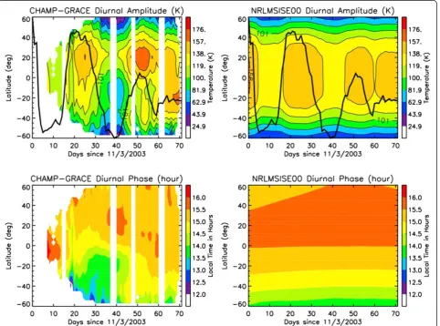
Some progress was also made in elucidating day-to-day tidal variability. Forbes et al. (2011) combined CHAMP and GRACE exosphere temperatures to perform daily tidal fits for selected time periods and found mainly solar-driven variability with a strong correlation with

the 27-day solar rotation period (Figure 6). Using com-bined WACCM-X/TIME-GCM simulations with constant solar and geomagnetic conditions but realistic tropospheric weather patterns, Liu et al. (2013a,b) showed day-to-day tidal amplitude variability on the order of 50% for the DW1, DE2, and DE3 tidal components in thermospheric winds, respectively. This in turn produced ExB vertical drift variability of the same magnitude and clearly indicates that tropospheric weather variability imposes a significant day-to-day variability on the ionosphere. At lower alti-tudes (mesosphere), Nguyen and Palo (2013) combined sounding the atmosphere using broadband emission radi-ometry (SABER) and microwave limb sounder (MLS) temperature data to derive day-to-day migrating diurnal tide variability at low latitudes and found amplitude changes of up to 15 K from one day to another. This is of the same order as variability deduced from‘ deconvolu-tion’approaches (Oberheide et al. 2002) using SABER alone (Figure 7). The causes for this variability still need to be

understood. It is not yet clear what the relative roles of tropospheric source variability and modulations imposed by wave-wave and wave-mean flow interaction processes are in causing this variability. Addressing this challenge is not only a matter of diagnosing short-term tidal variability from the data but will also require a concentrated effort by the modeling community. For example, a comparison of the diurnal tide in models and ground-based observations conducted as part of the 2005 equinox CAWSES tidal cam-paign (Ward et al. 2010) points to considerable differences in model magnitudes and vertical wavelengths suggesting that inconsistencies in model forcing, dissipation, and back-ground winds exist (Chang et al. 2012).

On longer time-scales, it has become clear that changes in global-scale weather patterns impose a considerable variability in the thermosphere and ionosphere. A compel-ling example that has recently attracted attention is the effect of the El Niño Southern Oscillation (ENSO). Pedatella and Forbes (2009a) found a high correlation between the

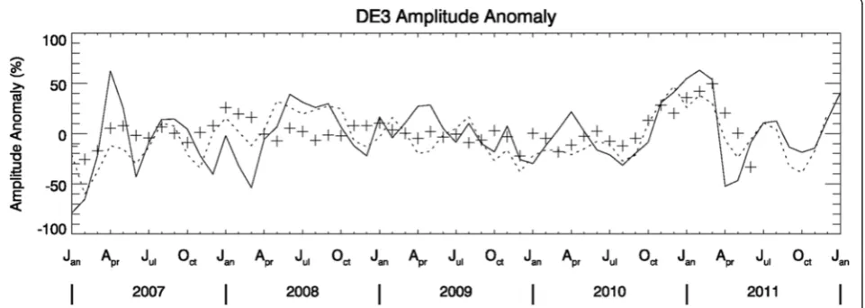
Oceanic Niño Index (ONI) and longitudinal foF2variability from low latitude ionosondes and associated this with ENSO-related changes in DE3 convective tidal heating. In a follow-up modeling study using WACCM, Pedatella and Liu (2012) showed that ENSO imposes a tidal temperature variability on the order of 10% to 30% during northern hemisphere winter. Interestingly, they found an enhanced DW1 and SW4 during the El Niño phase but a reduced DE2 and DE3. The latter components are enhanced during the La Niña phase. This is consistent with recent TIMED Doppler interferometer (TIDI) diagnostics focused on ENSO variability (Warner and Oberheide 2014). The ENSO-imposed variability is gener-ally smaller than the short-term tidal variability but similar to variability due to the quasi-biannual oscillation (QBO) determined by Oberheide et al. (2009). The ionospheric re-sponse to ENSO still needs to be studied in detail. A pre-liminary analysis (Figure 8) based on the COSMIC-based TEC tides from Chang et al. (2013) and the TIDI-, Tropical Rainfall Measuring Mission (TRMM)-, and Modern-Era

Retrospective Analysis for Research and Applications (MERRA)-based tidal wind and heating diagnostics from Warner and Oberheide (2014) indicates a consistent 50% enhancement in DE3 during the La Niña phase of the strong 2009 to 2011 ENSO and no response during the El Niño phase.

Tropospheric tidal forcing does not respond apprecia-tively to the solar cycle, and the E-region dynamo tidal winds remain more or less unaffected (Oberheide et al. 2009). In the thermosphere above 120 km, however, in-creasing background temperatures during higher solar activity cause more tidal dissipation because of the temperature dependence of thermal conductivity. For example, DE3 amplitudes during solar minimum are much larger than during solar maximum: a factor of 3 in the zonal wind, 60% in temperature and a factor of 5 in density (Oberheide et al. 2009; Häusler et al. 2013). On the other hand, relative TEC tidal amplitudes from COSMIC (Chang et al. 2013) do not show any solar cycle dependence. This can be understood as the result

Figure 8DE3 amplitude anomaly in TEC, E-region zonal wind, and tidal heating.DE3 amplitude anomaly (deviation with respect to the 2007 to 2011 climatological monthly means) in TEC (>200 km) from COSMIC at 15°N magnetic latitude (solid line), TIDI zonal winds at 100 km (averaged between 0°N to 20°N, dotted line), and TRMM- and MERRA-based convective and radiative DE3 heating, averaged from 3 to 16 km (plus symbols). Note the 50% enhancement in winter 2010/11 (La Niña phase) and the lack of any response in winter 2009/10 (El Niño phase).

of the absence of any solar cycle dependence in the zonal wind tides in the dynamo region which are the main driver of ionospheric tidal variability.

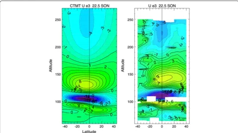
Connecting tides observed in the mesosphere lower thermosphere (MLT) region and those in the upper thermosphere and thus making the full connection to tropospheric weather from a purely observational point is still hampered by the lack of global wind or temperature observations in the‘thermospheric gap’ between TIMED observations (reliable below 110 km) andin situ observa-tions from satellites like CHAMP, GRACE, or the new Swarm mission at altitudes generally above 200 km. For example, much of the tidal characteristics in this height region rely on fits to TIMED observations such as the Cli-matological Tidal Model of the Thermosphere (CTMT, Oberheide et al. 2011a) that uses the observed tides in the MLT region as a constraint for a physics-based empirical model or general circulation models like WACCM-X (Liu et al. 2010a). The only dataset to date that turned out to be suitable for thermospheric tidal diagnostics came from HRDI and WINDII on UARS observations with tidal ‘deconvolution’applied (Lieberman et al. 2013a). Figure 9 exemplifies this for the DE3 using HRDI/WINDII diag-nostics from 60 to 250 km compared to CTMT. While CTMT does a reasonable prediction in this example, other components are not well reproduced, particularly DW2

and D0 that have additionalin situthermospheric sources, as shown by Jones et al. (2013) using the TIME-GCM. The existence of in situ thermospheric tidal sources for DW2 and D0 was confirmed by Forbes et al. (2014) who used the CTMT and combined CHAMP/GRACE tidal diagnostics to study tidal penetration to the upper thermosphere.

In continuation of the CAWSES-I tidal campaigns (Ward et al. 2010), TG4 continued the data analysis (e.g., Chang et al. 2012; Kishore Kumar et al. 2013) and conducted an additional campaign in August to October 2011. These campaign data still need to be analyzed and results will be published elsewhere. Although requiring a significant inter-national effort, observational campaigns such as these for various tropospheric and stratospheric conditions (ENSO, QBO) are important for developing and confirming our un-derstanding of tidal variability. See for example the recent modeling results by Gan et al. (2014) that highlight interan-nual variability in satellite-borne tidal diagnostics and in a general circulation model nudged to observed meteoro-logical reanalysis data. It should also be noted that tides provide the link between the‘weather’of the polar strato-sphere and ionospheric variability close to the geomagnetic equator, e.g., during sudden stratospheric warmings (SSW) as a result of planetary wave - tidal interaction. This is fur-ther elaborated on in project 3.

Project 2: What is the relation between atmospheric waves and ionospheric instabilities?

Equatorial plasma instabilities, commonly referred to as equatorial spread-F, plasma bubbles, or depletions can cause radio signals propagating through the disturbed region to scintillate resulting in a distortion or loss of signal. First observed by Booker and Wells (1938), they have been extensively studied due to the increasing im-portance of satellite-based communications and posi-tioning. Much has been learned over the decades about the growth mechanism and occurrence variability on a seasonal timescale. Dungey (1956) suggested the Rayleigh-Taylor instability as the generating process during post-sunset at the magnetic equator. At this time and location, since the bottom side of the F layer has recombined while the entire F layer itself has been raised by the pre-reversal enhancement, a very sharp vertical density gradient is cre-ated that is unstable to vertical perturbations in the iono-sphere. Identifying the contribution of atmospheric waves as a perturbation source and studying the resulting in-stabilities was the leading motivation for two observational campaigns carried out as part of TG4 activities.

The SpreadFEx-2 campaign

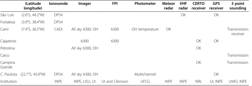
Based on the success of the first SpreadFEx campaign held in northeastern Brazil (e.g., Fritts et al. 2008), which focused on studying the interaction between the neutral atmosphere and ionosphere, especially during periods of ionospheric irregularities, a second set of campaigns, called SpreadFEx-2, was carried out in 2009 and 2010. A total of eight institutions participated in these campaigns, deploying instruments to the sites detailed in Table 3. The addition of the coherent electromagnetic radio tom-ography (CERTO) beacon receivers and deployment of multiple wide-angle imaging systems added the possibility of performing tomographic inversions of the ionosphere during periods of ionospheric irregularities while the de-ployment of Fabry-Pérot interferometers (FPIs) added the

capability to directly measure neutral winds and tempera-tures and study the relationship between the neutral and plasma state.

The campaigns were operated from early September until the end of November in both 2009 and 2010. These months correspond to the beginning of the ‘spread-F’ season, so called since this is when the occurrence of ionospheric irregularities (known as spread-F or equa-torial plasma bubbles) is more common. Combining data from the imaging systems and FPIs, the coupling of the neutrals and plasma during periods of equatorial plasma bubbles (EPBs) was studied. Chapagain et al. (2012) found that the zonal neutral winds and EPB zonal drift velocity, which is assumed to be indicative of the back-ground plasma drift velocity, were tightly correlated, es-pecially beginning several hours after sunset. The zonal velocities showed similar patterns of both nightly and night-to-night variability, indicating that the F-region dy-namo was fully developed. Earlier in the evening, how-ever, the EPB zonal speed was found to be slower than the background neutral winds, indicating that during the period of bubble development, the F-region dynamo might not be fully activated. Examples of the compari-sons made during the SpreadFEx-2 2009 campaign are shown in Figure 10. These examples show the overall similarity between the winds and EPB drift velocities as well as the variability in both of these parameters on a night-to-night basis. Histograms showing the differ-ence between the measured winds and estimated EPB drift velocities are shown in Figure 11 and show the good agreement between the two zonal speeds seen later in the evening (after 23 LT).

The data collection that begun under the SpreadFEx-2 campaigns has been continued through 2013, allowing for the study of the low latitude thermosphere through the transition from the deep solar minimum toward the solar maximum of solar cycle 24. A summary of the zonal and meridional thermospheric neutral winds as

Table 3 Spread FEx2 observation sites

(Latitude longitude)

Ionosonde Imager FPI Photometer Meteor radar

VHF radar

CERTO receiver

GPS receiver

3 point sounding

São Luís (2.6°S, 44.2°W) DPS4 OK OK

Fortaleza (3.9°S, 38.4°W) DPS4

Cariri (7.4°S, 36.5°W) CADI All sky 6300, OH 6300 OH temperature OK Transmission

receiver

Cajazeiras 6300 6300 OK OK

Petrolina All sky 6300, OH OK

Caico Transmission

Campina Grande

OK Transmission.

C. Paulista (22.7°S, 45.0°W) DPS4 All sky 6300, OH Multichannel OK

well as thermospheric neutral temperatures approxi-mately 250 km through the end of 2013 are presented in Figure 12. Analysis of the data collected through the end of July 2012 by Makela et al. (2013) showed the expected strong dependence of the neutral temperature on the solar flux, with the average temperature increasing by several hundred Kelvin over the study period. However,

a solar flux dependence was not seen in the neutral winds, at least over the range of solar fluxes observed during the period. Strong seasonal and day-to-day variability, however, is seen in the data indicating the influence of tidal and, possibly, gravity waves in the thermospheric neutral flows. The collection of this type of multi-year dataset will pro-vide important validation to models of the thermosphere

Figure 11Histogram of differences between the thermospheric neutral wind and equatorial plasma bubble drift velocities.Binned by local time. Total number of coincident observations in each bin is indicated by the blue line, referenced to the right hand axis.

and ionosphere being developed. Such a validation study for the WAM using the dataset that begun under the CAWSES SpreadFEx-2 campaign is presented in Meriwether et al. (2013).

The LONET campaign

The LONgitudinal NETwork (LONET) campaign was carried out as a TG4 activity during the September to November period in 2010 and 2011 with the goal of creating a robust, global, multi-instrument database to study the longitudinal variability of planetary-scale waves. Table 3 lists the observation sites and instrumenta-tion (13 ionosondes, 1 meteor radar, 2 MF radars, and 1 optical Fabry-Pérot interferometer) participating in LONET. TEC data obtained from the COSMIC satel-lite were also included. As can be seen from Table 4, the data collected in 2010 were more complete than 2011 in terms of the longitudinal coverage. Figure 13 shows the observation sites distributed along the equa-tor marked on a map. The rectangular boxes depict COSMIC TEC data sampling along the magnetic equa-tor. The ground-based data collection was limited in South America, Asia, and Oceania. No data were avail-able from the African continent.

As the first step in understanding the longitudinal variability of waves, the LONET team studied whether any global-scale periodic oscillations were present in the observed parameters and how the amplitude of those

oscillations varied with longitude. From the temporal variations of the ionospheric parameters foF2, h′F, TEC, and mesospheric winds, the 2- to 16-day oscillations were studied using wavelet analysis. In Figure 14, the wavelet power spectra for the three parameters, h′F at Fortaleza (FZA, 321.6°E), TEC at around 345°E, and MF radar zonal wind component at Pameungpeuk (107.7°E) are presented for the period consisting of day of year (DOY) 240 to 330. The h′F and TEC are approximately in the same longitudinal zone. Among the common os-cillations seen in these parameters is a distinct 16-day period oscillation during DOY 260 to 300.

In order to further investigate the 16-day oscillation, the amplitude and phase of the oscillation observed in the h′F parameter observed by the network of iono-sondes participating in the LONET campaign are plotted in Figure 15 for Fortaleza (FZA, top) to Darwin (DWN, second from the bottom). The mesospheric wind com-ponents (zonal winds at 89 km altitude), obtained from the MF radar at Pameungpeuk (PAM), are also shown (bottom) for reference. From the PAM wind oscillations in Figures 14 and 15, clear evidence of a 16-day oscilla-tion during the period DOY 260 to 320 centered at around DOY 290 is found. The h′F at Fortaleza shows clear 16-day oscillations during the same period with an amplitude that reaches approximately 4 km. However, the amplitudes of oscillation in the Indian and Asian sectors are somewhat lower compared to the American sites.

In Figure 16, we plot the results of a 16-day harmonic analysis of the COSMIC TEC data for different dinal zones. Each line corresponds to a given longitu-dinal zone, starting at 195°E (top) to 345°E (middle) to 165°E (bottom). During DOY 270 to 300, the 16-day os-cillation feature can clearly be seen. The phase of the maximum is slightly shifted from DOY 290 at 15°E to DOY 300 at 195°E, indicating that the phase is propagating westward. These observations suggest that the 16-day os-cillations might be generated by the Rossby mode 16-day planetary wave (Forbes 1995). Furthermore, there appear to be low amplitude regions (195 to 255°E) and high ampli-tude regions (315 to 105°E) in the global distribution of the oscillations. The Rossby 16-day waves normally appear in the troposphere to mesosphere mainly through the wind field and propagate into the lower thermosphere, modulat-ing the ionosphere (Lastovicka 2006). The present results provide further understanding regarding the latitudinal and longitudinal variability of the 16-day waves.

In addition to the ionospheric data presented above, data on geomagnetic field variations were also collected during the campaign period. The results of comparison with the ionospheric parameters will be presented else-where. Longitudinal variability of the spread F activity was also investigated using ground-based TEC observation over South America. Large day-to-day variability of spread

Figure 13Ground-based observation sites and COSMIC TEC data sampling areas along the geomagnetic equator for LONET campaign. Table 4 LONET campaign observation sites

Item Site Symbol Latitude Longitude 2010 2011 Contact

Ionosonde/foF2, h′F

1 Jicamarca JCM 12.0°S 76.9°W Partial YES Karim Kuyeng/Chau

2 Fortaleza FZA 3.9°S 38.4°W YES YES Inez Batista

3 C. Paulista CPT 22.7°S 45.0°W YES YES Inez Batista

4 São Luís SLS 2.5°S 44.3°W YES YES Inez Batista

5 Tirunelveli TIR 8.7°N 77.8°E YES NO Diwarker/Gurubaran

6 Gadanki GAD 13.5°N 79.2°E YES NO A.K. Patra

7 Cocos Islands COC 12.2°S 96.8°E YES YES Phil Wilkinson

8 Chumphon CPN 10.7°N 99.4°E YES NO Nagatsuma

9 Bac Lieu BCL 9.3°N 105.7°E YES NO Nagatsuma

10 Sanya SYA 18.3°N 109.6°E YES YES Guozhu Li

11 Wuhan WHN 30.5°N 114.3°E YES YES Guozhu Li

12 Cebu CEB 10.3°N 123.9°E YES NO Nagatsuma

13 Darwin DWN 12.5°S 130.9°E YES YES Phil Wilkinson

Meteor radar/wind

Jicamarca JCM 12.0°S 76.9°W Partial YES Luiz/Chau

MF radar/wind

1 Tirunelveli TIR 8.7°N 77.8°E Partial YES Narayanan/Gurubaran

2 Pameungpeuk PAM 7.6°S 107.7°E YES YES T. Tsuda/IUGONET

FPI (thermospheric winds)

Cairi CAR 7.5°S 36.4°W YES YES Makela/Meriwether

COSMIC satellite data (TEC)

F activity was observed, and the results were presented in the CAWSES TG4 News letter (vol. 7, page 5, 2012).

Progress of understanding for plasma bubble seeding by GWs

During the CAWSES-II interval, and in addition to the abovementioned campaigns, several additional interest-ing results were obtained relevant to the relation be-tween atmospheric waves and ionospheric instabilities. Takahashi et al. (2009) showed a positive correlation be-tween plasma bubble spacing and the spatial scale of mesospheric GW, which were observed simultaneously using airglow imagers in 630 nm and OH airglow emis-sions. Makela et al. (2010) found that the distribution of periodic spacing of equatorial plasma bubble compares favorably to the spectrum of GW-induced traveling iono-spheric disturbances (TIDs) measured by Vadas and Crowley (2010) from a similar geographic latitude in the northern hemisphere. These results suggest that the periodic spacing

of plasma bubbles are determined by GWs in the lower thermosphere. Several other studies also suggest seed-ing of plasma bubbles by GWs in the lower thermosphere (e.g., Taori et al. 2010, 2011; Paulino et al. 2011).

Distinct from these small-scale (approximately 100 km) GWs, large-scale wave structures (LSWSs, approximately 1,000 km) have been considered as another controlling factor of the plasma bubble/equatorial spread F (ESF) gen-eration (e.g., Tsunoda 2005). Thampi et al. (2009) and Tsu-noda et al. (2010) demonstrated that a close relationship exists between LSWS and the generation of ESF when the post-sunset rise (PSSR) of the F layer was absent. Tsunoda et al. (2011) showed that the amplification of LSWS in the late afternoon mostly occurs during the post-sunset rise of the equatorial F layer. Narayanan et al. (2014) showed that the occurrences of ionogram satellite traces, which are used as a proxy of LSWS, were followed by ESF in about 71% of the cases, supporting the view that LSWS appears to be an important parameter in the formation of ESF.

It is also interesting to note that Otsuka et al. (2012) and Shiokawa et al. (2014) reported observations of the dissipation of plasma bubbles in the field-of-view of 630 nm airglow images due to collision of the bubbles with a mid-latitude MSTID and a large-scale TAD, respectively. In both cases, the bubbles seem to be dissipated by polarization electric field associated with these waves in the ionosphere and thermosphere. This process sug-gests an additional role of GWs in the ionosphere, namely the suppression of ionospheric instabilities.

Project 3: How do the different types of waves interact as they propagate through the stratosphere to the

ionosphere?

A variety of satellite- and ground-based data sets along with model simulations have been used during the CAWSES-II time frame to delineate how large-scale waves propagate through the middle atmosphere to the ionosphere. Several dedicated campaigns, e.g., coordinated ISR observations

during SSWs, and workshops (Table 2) involved the TG4 community and were supported by TG4.

PW signatures in the ionosphere

For example, the global distribution and the climato-logical features of the 5- to 6-day planetary waves de-rived from SABER/TIMED temperature measurements over the height range 20 to 120 km for a full 6-year period were delineated by Pancheva et al. (2010). This study determined that the 5-day wave, the gravest sym-metric wave number 1 Rossby wave, has a vertically propagating phase structure with a mean vertical wave-length of approximately 50 to 60 km, whereas the 6-day wave is an equatorially trapped wave number 1 eastward propagating wave with a mean vertical wavelength of ap-proximately 25 km. Liu et al. (2010a,b) attributed tem-poral hmF2‘wave-4’variations diagnosed from COSMIC

Figure 1516-day period oscillations of h′F and mesospheric winds.16-day period oscillations of h′F and mesospheric winds (bottom) during the LONET campaign period in 2010.

data to the interaction of the DE3 with the 5- and 2-day planetary waves. In another study, Mukhtarov et al. (2010) reported on the climatology of stationary planet-ary waves with zonal wave numbers 1 and 2 observed in SABER/TIMED temperatures for the same period. Further, using COSMIC data on ionospheric parameters, foF2and hmF2 and electron density at fixed altitudes and the SABER temperature data, Pancheva and Mukhtarov (2012) diagnosed the global-scale spatial and temporal variability of the approximately 23-day zonally symmetric planetary wave during the Northern winter of 2008/2009. The iono-spheric oscillations were shown to be forced by planetary waves propagating from below. Pedatella and Forbes (2009b) demonstrated the presence of 16-day waves that were simultaneously observed in the CHAMP electron densities at 350 km, total electron content from global positioning system (GPS) observations, and in SABER temperature data at altitudes of 110 km, indicating that vertically propagating planetary waves induce signifi-cant variability in the low latitude F-region ionosphere and that these effects are seen at all longitudes. Re-cently, Chang et al. (2013) analyzed COSMIC TEC data and found strong stationary planetary wavenum-ber 4 (SPW4) signals (Figure 17), most likely caused by a strong SPW4 in neutral zonal wind in the E-region (Oberheide et al. 2011b) that in turn is the result of a modulation of the migrating diurnal tide DW1 by the DE3 nonmigrating tide (Hagan et al. 2009).

While the presence of PW signatures in the iono-spheric plasma is without dispute and the same neutral/ plasma coupling processes as for the tides (predominantly E-region dynamo modulation, see project 1) are thought to apply to PWs as well, the mechanism through which they enter the E-region is still under debate. For example,

planetary waves do not penetrate much above 100 km, but instead are thought to impose their periodicities on the ionosphere and thermosphere by modulating the tides and gravity waves that do penetrate to higher altitudes. Other mechanisms include secondary PW forcing. For in-stance, Lieberman et al. (2013b) using MLS, SABER, and TIDI data, along with Navy Operational Global Atmos-pheric Prediction System - Advanced Level Physics-High Altitude (NOGAPS-ALPHA) model simulations found observational evidence for wintertime SPWs in the lower thermosphere forced in part by drag imparted by gravity waves that have been modulated by underlying strato-spheric SPWs. Their results supported earlier model and case studies by Liu and Roble (2002), Smith (2003), and Oberheide et al. (2006a) that already suggested the plausibility of this mechanism.

SSW impact on the ionosphere and thermosphere

A prime example for tidal modulation by PWs occurs during sudden stratospheric warmings. An SSW is an extreme atmospheric disturbance event that results in a warmer polar stratosphere and reversed zonal mean flow at mid-latitudes and provides the link between the ‘weather’ of the polar stratosphere and ionospheric variability close to the geomagnetic equator. As a consequence of publica-tion of the observapublica-tional evidence for the ionospheric sig-natures associated with a SSW event by Goncharenko and Zhang (2008), several studies in the recent past have ad-dressed the effect of SSW on the ionosphere due to planet-ary wave propagation from below. It is now understood that the planetary waves modulate the propagation charac-teristics of predominantly the semidiurnal migrating tide, enhancing its amplitude, and thereby modulating the E-region ionospheric dynamo, vertical plasma drifts,

and plasma density in the F-region, in a manner simi-lar to the effects of nonmigrating tides (Liu et al. 2010b; Fuller-Rowell et al. 2011; Chau et al. 2012; Jin et al. 2012). This is exemplified in Figure 18 in which GAIA model simulations are compared with COSMIC and SABER satellite observations during the January 2009 SSW.

A recent ground-based study by Laskar et al. (2014) conducted in the Indian sector suggests that the 16-day modulation of the semidiurnal tide is particularly strong during strong SSW events and as such exerts a signifi-cant impact on ionospheric variability even during high solar activity. Although SSWs only happen at most a few times per year, they nevertheless provide an excellent opportunity to test current theories of neutral-plasma coupling on a global scale and for testing the predictive capabilities of space weather models, as SSWs can be forecasted on a 1-week timescale (Fuller Rowell et al. 2011; Wang et al. 2014).

Pancheva and Mukhtarov (2011) presented for the first time the global spatial (latitude and altitude) structure of the mean ionospheric response to SSW events during winters of 2007/2008 and 2008/2009 using COSMIC foF2 and hmF2 and electron density data at fixed altitudes. Several studies were carried out to understand the pro-cesses underlining the SSW control of the electrodynamics

at low latitudes. Chau et al. (2009) provided strong evidence indicating that the distinctive behavior of the vertical ExB drifts over the magnetic equator during daytime was associ-ated with a minor SSW. Following this work, Chau et al. (2010) identified SSW signatures in several ionospheric pa-rameters using the incoherent scatter radar (ISR) elec-tron density and temperature measurements from the Arecibo Observatory, as well as relative TEC variations derived from a dual-frequency GPS receiver. To examine the response of the mid-latitude ionosphere to SSW, Goncharenko et al. (2013) undertook a case study of the day-to-day variability in the ion temperature at alti-tudes between 200 and 400 km and detected disturbances at tidal periods as well as at non-tidal and multi-day pe-riods. As planetary waves are not expected to reach mid-dle and upper thermospheric altitudes, as noted in the previous subsection, these results have once again raised questions about the underlying mechanisms coupling the lower and upper atmosphere.

A TIME-GCM simulation by Liu and Roble (2002) re-vealed that the resonant SPW amplification prior to the peak warming causes a deceleration of the mean wind in the high latitude winter stratopause and mesosphere and reverses to westward with a critical layer near the zero wind line. This changes the filtering of gravity waves by allowing more eastward GW to propagate into the MLT

region and a resulting change of the meridional circula-tion in the upper mesosphere from poleward/downward to equatorward/upward with corresponding stratospheric warming, mesospheric cooling, and thermospheric warm-ing patterns in the mean temperatures at high latitudes during SSWs. At low latitudes, this temperature pattern reverses and produces a thermospheric cooling and conse-quently a thermospheric density decrease at a fixed alti-tude by reducing the scale height.

SSW and lunar tides

Recent ground-based and satellite magnetometer observa-tions in conjunction with other ionospheric measurements have provided insights of how lunar tidal modulation dur-ing SSW events can drive the spatio-temporal variabilities of the equatorial electrojet and the electrodynamics (Fejer et al. 2010, Park et al. 2012, Yamazaki et al. 2012). How-ever, Stening (2011) argued against a strong lunar tidal contribution to the observed variability during SSWs since strong lunar tidal signals exist during non-SSW periods so that these correlations might be coincidental. Fuller-Rowell et al. (2011) indeed found SSW-induced phase shifts in the semidiurnal solar tide consistent with an apparent lunar tidal signal using WAM simulations, but it should be noted that the model did not include the semidiurnal lunar tide as an input. Wang et al. (2014) in a coupled WAM/iono-sphere model simulation also found a phase shift of the SW2 solar component during SSWs caused by SSW-induced variability in its main source, stratospheric ozone, and/or additional middle atmosphere circulation changes. On the other hand, Pedatella et al. (2014) reported notable enhancements of the semidiurnal lunar tide during SSW events in WACCM-driven TIME-GCM simulations and a better agreement with COSMIC electron density observa-tions when the lunar tide was included in the model. It must thus be concluded that the impact of lunar tides on ionospheric variability during SSWs is not yet finally re-solved and requires further studies by the aeronomy com-munity over the coming years. It should also be noted that there is increasing evidence that the ionospheric plasma variability during SSWs is not solely caused by E-region electric field variability but also by variability in F-region meridional neutral winds and thermospheric composition changes (e.g., Pedatella et al. 2014). This is consistent with the earlier modeling work by England et al. (2010) and Maute et al. (2012) that was focused on nonmigrating tides.

SSW and GW

Small-scale variability of the upper atmosphere driven by major atmospheric disturbances from below like SSW has also gathered attention recently. Adopting a first principle nonlinear hydrostatic GCM extending from the lower atmosphere to the thermosphere, Yiğit et al.

(2014) investigated the influence of small-scale gravity waves originating in the lower atmosphere on the vari-ability of the high latitude thermosphere during an SSW event. The numerical experiments revealed that the gravity wave penetration into the thermosphere in-creased the momentum deposition rates above 150 km in the high latitude northern hemisphere by up to a factor of 3 to 6 during the warming. This demonstrates that gravity wave-induced variations during SSWs con-stitute a significant source of high latitude thermospheric variability.

Project 4: How do thermospheric disturbances generated by auroral processes interact with the neutral and ionized atmosphere?

Upper thermosphere

From the CHAMP satellite observations, Lühr et al. (2004) showed the existence of strong heating in the cusp (and/or near the cusp) region. This heating causes upwell-ing of the air and enhancement of the neutral mass dens-ity in the altitude region of about 400 km. In addition, the CHAMP satellite observed some thermospheric distur-bances during geomagnetically disturbed periods. For ex-ample, Ritter et al. (2010) identified substorm-related thermospheric density and wind disturbances from the CHAMP observations. They reported mass density en-hancements, a density bulge propagating as a traveling at-mospheric disturbance (TAD), and wind variations during a substorm event. Liu and Yamamoto (2011) reported geomagnetic storm effects on the formation and charac-teristics of the mid-latitude summer nighttime anomaly (MSNA), which is a phenomenon during which the diur-nal variation of the plasma density maximizes at night in-stead of day. They pointed out the role of the effective neutral wind in the formation of MSNA. Some results ob-tained from the CHAMP observations were summarized in the review paper presented by Lühr et al. (2012).

Vickers et al. (2013) developed a new technique to ob-tain thermospheric neutral density at approximately 350 km altitude from incoherent scatter radar data. In situ comparisons with the CHAMP satellite show good agree-ment. Vickers et al. (2014) used this technique on the EIS-CAT Svalbard radar for the period 2000 to 2013 and showed that F10.7 solar irradiance is a very good proxy for thermospheric density variations with only a small sea-sonal dependence. In addition, the long-term trend of de-clining thermospheric density was observed.

wind streams from the DMSP F13 satellite observations and the Thermosphere-Ionosphere-Electrodynamics General Circulation Model (TIE-GCM) simulations. They concluded that the disturbance dynamo would be an important mech-anism for driving the electrodynamic response at dawn and dusk to recurrent geomagnetic activity driven by HSS. Gardner et al. (2012) investigated the HSS heating effects from numerical simulations and observations with the EIS-CAT Svalbard radar (ESR) and PFISR. They showed that the HSS heating can cause temperature enhancement as high as 100 K at high latitudes, but the global increase in thermo-spheric temperature would be low.

Coronal mass ejections (CMEs) are also one of the im-portant causes of the geomagnetic storms. The thermo-spheric density variations during CME- and CIR-induced geomagnetic activities were compared by Chen et al. (2012). The total changes in the thermospheric density ob-served during periods of CIR storms were greater than those of the CME storms because the CIR storms lasted longer than CME storms, while the CME storms were stronger than the CIR storms on average.

For smaller scale waves, several airglow imagers inves-tigated thermospheric and ionospheric waves identified as MSTIDs near the auroral zone through the 630 nm airglow emissions at altitudes of 200 to 300 km. Kubota et al. (2011) reported characteristics of MSTIDs ob-served by an airglow imager at Alaska. They concluded that these southwestward-moving MSTIDs are not caused by ionospheric instabilities, as usually suggested at middle latitudes, but are likely to be caused by auroral distur-bances as TADs because the observed background ther-mospheric wind was poleward, stabilizing the ionospheric instability. On the other hand, Shiokawa et al. (2013) reported similar southwestward-moving MSTIDs over Norway and northern Canada and suggested that they are caused mainly by the Perkins and E-F coupling in-stabilities (Perkins 1973; Yokoyama et al. 2009) similar to those at middle latitudes and that an additional source by atmospheric gravity waves from lower altitudes also comes into play. Shiokawa et al. (2012, 2013) reported sudden movements of these MSTIDs at subauroral lati-tudes concurrent with auroral activity, indicating instant-aneous penetration of auroral electric fields to subauroral latitudes.

MLT region

Dynamics and Energetics of the Lower Thermosphere in Aurora (DELTA) and DELTA-2 campaigns were carried out in December 2004 and January 2009, respectively. Simultaneous observations with the EISCAT radar, FPI, and sounding rockets were successfully made during the two campaigns. For example, Kurihara et al. (2009) iden-tified temperature enhancement in the lower thermo-sphere in association with the auroral heating during the

DELTA campaign. Oyama et al. (2010) also reported lower thermospheric wind fluctuations measured with an FPI during pulsating aurora at Tromsø, Norway, in the period of the DELTA-2 campaign (Figure 19). Some studies con-cerning the occurrence of atmospheric gravity waves in the polar thermosphere in response to auroral activity were summarized in the review paper of Oyama and Watkins (2012).

Following initial studies of thermospheric meso-scale variability using tristatic Fabry-Pérot interferometer (FPI) observations at EISCAT (Aruliah et al. 2004, 2005), the neutral wind variations in the vicinity of an auroral arc were studied by some researchers. Oyama et al. (2009) showed spatial evolution of frictional heating and in-creases in ion flow and temperature in the vicinity of an auroral arc from observations with the Sondrestrom incoherent-scatter radar and the Reimei satellite. They clarified localized ionospheric structures associated with localized soft particle precipitation or F-region ionization, suggesting the presence of a narrow thermospheric wind shear of about 10 km width. Kosch et al. (2010) reported the first observational results of the E-region neutral wind fields and their interaction with auroral arcs during geo-magnetically quiet conditions at Mawson, Antarctica, with a scanning Doppler imager (SDI). The 144° field-of-view Doppler images of the sky over Mawson are shown in Figure 20. They found that E-region wind could rotate 90° within approximately 10 min when close to (within approximately 50 km) of an auroral arc and then recover to the background flow when the arc disappeared. The F-region wind remained unaffected. This was attrib-uted to the electric field associated with auroral arcs caus-ing localized strong ion drag. Anderson et al. (2011) performed bistatic FPI observations of F-region ther-mospheric vertical winds in Antarctica. They found strong upward winds poleward of the auroras as well as correlated vertical wind responses over horizontal distances of approximately 150 to 480 km.

neutral wind dynamo contribution to Joule heating was 36% to 64% on average and was positive when the hori-zontal magnetic field perturbation was weak (|ΔH| < approximately 40 nT) and vice versa. They estimated the F-region ion - neutral collision frequency at 260 km altitude using the ambipolar diffusion equation - and also found good agreement with the MSIS model.

Recently, Xu et al. (2013) showed longitudinal varia-tions of the thermospheric temperature from satellite observations with SABER and Michelson Interferometer for Passive Atmospheric Sounding (MIPAS) and simula-tions with TIE-GCM. Their simulasimula-tions clarified that

auroral heating would cause the observed longitudinal temperature variations. In addition, the satellite obser-vations indicated that impacts of auroral heating on the neutral atmosphere can penetrate down to about 105 km. The lidar observations are quite useful to study thermospheric disturbances in the MLT region. For example, Chu et al. (2011) observed temperature enhancements caused by Joule heating and fast gravity waves propagating from the lower atmosphere in the neutral Fe layers (110 to 155 km) in Antarctica. Tsuda et al. (2013) showed decreases in sodium density in as-sociation with auroral particle precipitation from

simultaneous and common volume observations by the EISCAT VHF radar and a sodium lidar at Tromsø, Norway.

Model simulations in association with auroral/high latitude phenomena

Some general circulation models (GCMs) have been devel-oped to understand the energetics, dynamics, and compos-ition variations of the upper atmosphere. These simulations clarified disturbances in the polar ionosphere and thermo-sphere in association with auroral activity and/or high lati-tude energy inputs. For example, Qian et al. (2010) simulated thermospheric response to recurrent geo-magnetic forcing with the NCAR TIE-GCM. Neutral density and nitric oxide (NO) cooling rates were simu-lated for the declining phase of solar cycle 23. The simulated results were compared to neutral density de-rived from satellite drag and to NO cooling measured by TIMED/SABER. Gardner and Schunk (2011) per-formed numerical simulations to investigate character-istics of the large-scale gravity waves with a high-resolution global thermosphere-ionosphere model which can represent global distributions of mass density, temperature, and all three components of the neutral wind at altitudes from 90 to 500 km without the assumption of hydrostatic equilib-rium. They noted that a secondary wave was generated

which propagated around the entire globe, while the original gravity wave was localized. Deng et al. (2011) also investi-gated nonhydrostatic effects in the thermosphere from Global Ionosphere Thermosphere Model (GITM). Their simulations demonstrated that most of the nonhydrostatic effects at high altitudes (300 km) arise from sources below 150 km and propagated vertically through the acoustic wave. Basic structures of the polar ionosphere and thermosphere during solar minimum and geomagnet-ically quiet periods were investigated by Fujiwara et al. (2012) from the EISCAT Svalbard radar observations (March 2007 to February 2008) and simulations with a whole atmosphere GCM. Their results indicated that both the ions and neutrals would show larger varia-tions than those described by the empirical models, suggesting significant heat sources in the polar cap re-gion even under solar minimum and geomagnetically quiet conditions. In addition to the global model simu-lations, de Larquier et al. (2010) performed one- and two-dimensional numerical simulations with a finite-difference time-domain (FDTD) model to provide quantitative inter-pretation of the recently reported infrasound signatures from pulsating aurora. They discussed pressure perturba-tions caused by particle heating due to pulsating aurora (heat source is located between 90 and 110 km on aver-age). The simulation results were roughly an order of

Figure 21The spatial distribution of Joule heating in 22.5° sectors.The spatial distribution of Joule heating in 22.5° sectors about the EISCAT Svalbard radar projected to 110 km 23:36 to 23:54 UT on 2 February 2010. The aurora (areas in green color) is overlaid for 110 km altitude. (See figure on previous page.)

magnitude smaller than those observed, suggesting the need for an additional source, e.g., Joule heating.

Conclusions

Scientific outcome and challenges

Overall, TG4 brought together the historically separate neutral atmosphere and plasma communities in a way that allowed for much progress in understanding how neutral variability originating in the lower atmosphere impacts and interacts with Earth's ionosphere, from low to polar latitudes and from the troposphere to the F-region. For example, the role of waves due to con-vection, polar stratosphere dynamics, or auroral processes in causing substantial ionospheric variability through dy-namo processes and Rayleigh-Taylor instabilities is now much better understood than before. This was achieved through a combination of dedicated campaign activities and workshops resulting in four special issues in the peer-reviewed literature (Table 2). The aeronomy community is well on its way to separating ionospheric variability intro-duced by driving from below and from the magnetosphere and Sun above, an essential task toward achieving predict-ability of space weather. In this respect, it is important to note that the solar activity at the beginning of the CAWSES-II period was extremely quiet, allowing the pure effects from the lower atmosphere to be observed in isolation without disturbances from above.

There are a number of critically important open questions toward the goal of achieving space weather predictability. Significant amounts of variability remain unexplained and/ or are very difficult to detect and interpret, for example, the imprints of convectively forced gravity waves in the thermo-sphere. Short-term tidal variability in the neutrals and plasma is largely unknown because of the lack of suitable satellite data since local time coverage by a single satel-lite is limited. It is not clear what is more important: wave propagation into the thermosphere and then into to the ionosphere; or electrodynamic coupling between the E- and F-region and then into the thermosphere. The dynamics community still knows little about inter-actions between the various types of waves (tides, PWs, and GWs) and the mean flow. A major observational and technological challenge is the lack of global wind observa-tions, day and night, throughout the 120 to 400 km region.

As overviewed below, new space-borne and ground-based assets, along with progress in geospace modeling, will help to close this knowledge gap that is also targeted through elements of SCOSTEP's new VarSITI program.

Program outreach

As a dedicated effort of the international scientific com-munity, and in accordance with SCOSTEP's mission not only to run scientific programs but also to promote solar-terrestrial physics and dissemination of the derived

knowledge for the benefit of society, Task Group 4 pub-lished a quarterly newsletter. Each newsletter was about eight pages long with updates on recent campaign activ-ities, short news, and a portrait of a young scientist. All ar-ticles were written to be understandable for non-specialist and published on the task group wiki (www.cawses.org/ wiki/index.php/Task_4) and through an extensive mailing list. A total of 13 issues have been published with 64 arti-cles from authors from 20 different countries, including 10 articles featuring young scientists. TG4 also organized and/or supported 12 dedicated workshops and special ses-sions and held annual business meetings during major conferences.

New and future satellite missions

Space agencies and national science foundations in the U.S., Europe, and Asia by now recognize the importance of lower atmosphere driving of the ionosphere-thermosphere system not only as a domain of compelling scientific inquiry but also as highly relevant for understanding and predicting space weather; a task highly relevant for technological societies.

In the United States, the Decadal Survey on Solar and Space Physics 2013 to 2022 conducted by the National Academy of Sciences (National Research Council 2013) recognized the realization that weather systems in the troposphere impact space weather through tides and gravity waves as one of the significant discoveries in the past decade, making ‘the comprehensive understanding of the variability in space weather driven by lower-atmosphere weather on Earth’its second highest priority and recommended a dedicated satellite constellation (DYNAMIC) to be launched around the year 2020. While NASA budget constraints may delay the imple-mentation of DYNAMIC; two new satellite missions dedicated to ionosphere-thermosphere physics, ICON and GOLD, will be launched in 2017. Both ICON and GOLD can be seen as pathfinder missions for DY-NAMIC. ICON will collect data from a low Earth orbit to compare the impacts of direct solar driving and lower atmosphere driving on variability in the ionosphere/ thermosphere system, and GOLD will image the thermo-sphere from a geostationary orbit, allowing for an unprece-dented global view of short-term variability.

Langmuir probe, an accelerometer, and GPS instrumenta-tion on board, similar to the tremendously successful CHAMP satellite. During its anticipated 10-year mission, the Swarm data will allow the ionosphere/thermosphere community to obtain an unprecedented view of small-scale structures in the thermosphere and the ionospheric plasma.

Due to the success of COSMIC (a particularly important dataset for the ionosphere/thermosphere community be-cause of its global electron density profiles from radio occult-ation), the United States and Taiwan will launch COSMIC-2 between 2015 and 2018. COSMIC-2 consists of six satellites in a low-inclination orbit (launch in 2015) and another six satellites in high inclination orbits (launch in 2018).

Along with emerging cubesat and nanosat capabilities, these new space-borne assets will form the backbone of studying the signatures and impact of lower atmosphere variability versus magnetosphere/solar-driven variability in the next decade. Their synergistic use will most likely allow the community to make significant progress ward understanding geospace as a system and also to-ward predictability of space weather, a significant need for a technological society. A particular challenge, how-ever, will remain: global thermospheric winds through-out the whole thermosphere during day- and nighttime; dataset airglow interferometers cannot provide. The im-plementation of new emerging technologies, such as the Doppler wind and temperature sounder (DWTS; Gordley and Marshall 2011; Lieberman et al. 2012), will be needed.

New ground-based assets

Ground-based facilities are powerful tools to measure ver-tical coupling from the atmosphere to geospace. They are basically radio techniques (various types of radars, iono-sondes, satellite beacon receivers including Global Naviga-tion Satellite System (GNSS) receivers, natural/artificial wave receivers, and magnetometers) and optical tech-niques (imagers and interferometers for airglow and aur-ora; and lidars). Figure 22 summarizes the altitude ranges and measurement parameters of various ground-based techniques. Because a single instrument covers only a certain range of altitudes and can measure a limited set of physical parameters, it is essential to combine several types of instruments at the same place to under-stand the connection from the troposphere to geospace. Multi-point networks of these various instruments are becoming available, providing global information of these parameters, e.g., Yumoto (2011) - MAGDAS and Yizengaw and Moldwin (2009) - AMBER for magne-tometers, Makela et al. (2009) - RENOIR, Shiokawa et al. (2009) - OMTIs, Makela et al. (2012) - NATION, and Meriwether et al. (2014) - Peruvian FPIs for op-tical instruments, and Cohen et al. (2010) - AWESOME for LF/VLF receivers. It is also important to combine these ground-based observations with satellite measurements to separate temporal and spatial variations.

One of the great progress of ground-based observation during CAWSES-II was that the multi-point GNSS re-ceiver network is becoming a powerful tool to provide