Estimating range of influence in case of missing spatial data: a simulation study on binary data

INTERNATIONAL JOURNAL OF HEALTH GEOGRAPHICS Bihrmann and ErsbøllInternational Journal of Health Geographics2015,14:1

http://www.ij-healthgeographics.com/content/14/1/1

M E T H O D O L O G Y

Open Access

Estimating range of influence in case of missing

spatial data: a simulation study on binary data

Kristine Bihrmann

and Annette K Ersbøll

Abstract

Background: The range of influence refers to the average distance between locations at which the observed outcome is no longer correlated. In many studies, missing data occur and a popular tool for handling missing data is multiple imputation. The objective of this study was to investigate how the estimated range of influence is affected when 1) the outcome is only observed at some of a given set of locations, and 2) multiple imputation is used to impute the outcome at the non-observed locations.

Methods: The study was based on the simulation of missing outcomes in a complete data set. The range of influence was estimated from a logistic regression model with a spatially structured random effect, modelled by a Gaussian field. Results were evaluated by comparing estimates obtained from complete, missing, and imputed data.

Results: In most simulation scenarios, the range estimates were consistent with≤25% missing data. In some scenarios, however, the range estimate was affected by even a moderate number of missing observations. Multiple imputation provided a potential improvement in the range estimate with≥50% missing data, but also increased the uncertainty of the estimate.

Conclusions: The effect of missing observations on the estimated range of influence depended to some extent on the missing data mechanism. In general, the overall effect of missing observations was small compared to the uncertainty of the range estimate.

Keywords: Range of influence, Missing data, Binary data, INLA

Background

In spatial data, the range of influence refers to the average distance between locations at which the observed out-come is no longer correlated. The range of influence can be estimated from a variogram or based on a regression model with a spatially structured random effect, modelled by a Gaussian field. Traditionally, the regression model has posed a computational challenge in all but very small data sets, due to the need to invert a dense covariance matrix. However, the recent development of the so-called stochastic partial differential equation (SPDE) approach [1] along with the Integrated Nested Laplace Approxima-tion (INLA) [2] approach to Bayesian inference have made these models computationally feasible. The SPDE links the Gaussian field to a Gaussian Markov random field given

*Correspondence: [email protected]

1Faculty of Medical and Health Sciences, University of Copenhagen, Grønnegårdsvej 8, DK-1870 Frederiksberg C, Denmark

Full list of author information is available at the end of the article

by a sparse precision matrix, and INLA is a computation-ally efficient alternative to MCMC for Bayesian inference, particularly since no sampling is required. Regression models with a spatial component could be applied in sev-eral different settings where modelling a spatial pattern is of interest. Examples include rainfall in a geographic area and pricing of houses, as well as health, disease, and lifestyle outcomes, for example the spread of an infectious disease.

Many (if not the majority of ) studies are subject to miss-ing data. For example, the price of a house is only known if the house has been sold within the study period. Similarly, all studies based on survey data will only include informa-tion on those who participated in the survey. This study will focus on the situation where a binary outcome, dis-ease status for example, is missing at some of a given set of locations.

Missing data are often classified in three categories [3]: 1) missing completely at random (MCAR): the probability

Bihrmann and ErsbøllInternational Journal of Health Geographics2015,14:1 Page 2 of 13 http://www.ij-healthgeographics.com/content/14/1/1

of data being missing does not depend on the observed or the unobserved data, 2) missing at random (MAR): the probability of data being missing does not depend on the unobserved data, conditional on the observed data, and 3) missing not at random (MNAR): the probability of data being missing does depend on the unobserved data, conditional on the observed data. This categorisa-tion is based on assumpcategorisa-tions about the missing data and cannot be tested. It is well-known that missing data can cause biased and/or inefficient estimates of, for example, regression parameters and standard errors - if not han-dled adequately. A popular tool for handling missing data is multiple imputation (MI) [4], at least if the missing data are not MNAR. In MI, the distribution of the observed data is used to estimate a set of values of the missing data. To our knowledge, the effect of missing data (and in particular missing outcomes) on the estimated range of influence has not been studied.

The objective of this study was to investigate how the estimated range of influence is affected when 1) a binary outcome is only observed at some of a given set of loca-tions, and 2) multiple imputation is used to impute the outcome at the non-observed locations. For simplicity, complete information on covariates was assumed. The investigation was based on the simulation of missing data in a complete data set with known locations.

Results and discussion

The range of influence was estimated to 12.7 km (stan-dard deviation (SD) 4.4) in the complete data set. All the reported analyses included the only significant covariate ((log-) herd size) in the regression model. The estimation was based on a triangulation of the considered region, and a finer triangulation did not change the estimate, but did markedly increase computing time. Reducing the region to make the shape of the area more regular slightly decreased the estimated range of influence. A sensitivity analysis to determine the effect of the prior distribution of the hyperparameters showed no effect on the estimates obtained from the complete data. With missing data, the range estimate did not change when increasing the pre-cision of the prior from 0.00001 to 0.001. In the majority of missing data scenarios, however, a precision of 0.1 pro-duced a range estimate further from the estimate obtained from the complete data, as well as a larger standard devi-ation, compared to the results obtained with precision 0.001. The maximum difference in median range within scenarios was 1 km, and in most scenarios it was less than 0.5 km. These differences are small considering the uncertainty of the range estimate. They do, however, indi-cate that a precision of 0.1 was a potentially informative prior when the information within the data was reduced by missing observations. Therefore, a prior with precision 0.001 was preferred in the analyses. As a consequence,

however, various computational problems were encoun-tered with 75% missing data. These problems were solved by simply changing the precision to the default value of 0.1. This was done in all analyses of data sets with 75% missing data, and the results may not, therefore, be fully comparable to scenarios with fewer missing observations. The same computational problems were encountered with both 50% and 75% imputed data. In these scenarios, the precision 0.1 was also used. Overall, the variance param-eter σ2 (part of the spatial covariance function) was unaffected by the prior distribution.

As part of the INLA procedure used to estimate param-eters, eigenvalues of a Hessian matrix are computed. Neg-ative eigenvalues, which may affect the accuracy of the approximation, were seen in three simulation scenarios (MAR0 OR=3, MAR1 OR=3, and MNAR OR=1/3; simula-tion scenarios are described in the Methods secsimula-tion) when 50% or more of the observations were missing. This hap-pened in only 1 or 2 out of 1000 data sets. In imputed data, the problem was slightly more evident, especially with 75% imputed data where on average it happened in three out of 1000 data sets. Due to the limited extent, however, the problem was disregarded.

In some of the incomplete data sets, an unrealistically large estimate of the range of influence was obtained, e.g. 360 km - despite the maximum distance between loca-tions being only 76 km. A large range estimate is the result of a small estimate of the scaling parameterκin (5), which means the correlation between locations decreases slowly with increasing distance. Hence, an estimated range of influence that extended beyond the observed data was interpreted as an essentially constant correlation within the observed data, i.e. there was no detectable spatial cor-relation present. The situation corresponds to obtaining a flat variogram. In the overall results of the simulation study (Tables 1 and 2), data sets with an estimated range of influence larger than 75 km were excluded. Furthermore, medians (rather than means) were used to summarise the simulation results.

Missing data

Bihrmann

and

E

rsbøll

International

Journal

o

fH

ealth

G

eographics

2015,

14

:1

Page

3

o

f

1

3

http://www.ij-healthgeographics.com/content/14/1/1

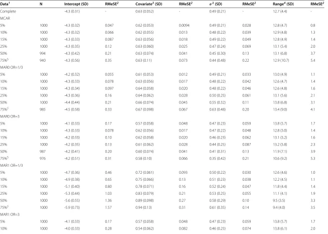
Table 1 Summary of parameter estimates obtained from complete and simulated missing data

Data1 _{N Intercept (SD) RMeSE}2 _Covariate3_{(SD) RMeSE}2 _σ2_{(SD) RMeSE}2 _Range4_{(SD) RMeSE}2

Complete -4.3 (0.31) - 0.63 (0.052) - 0.49 (0.21) - 12.7 (4.4)

-MCAR

5% 1000 -4.3 (0.32) 0.047 0.62 (0.053) 0.0094 0.49 (0.21) 0.028 12.8 (4.7) 0.8

10% 1000 -4.3 (0.32) 0.066 0.62 (0.055) 0.013 0.48 (0.22) 0.039 12.9 (4.8) 1.3

15% 1000 -4.3 (0.33) 0.087 0.63 (0.056) 0.018 0.49 (0.22) 0.049 12.8 (4.9) 1.4

25% 1000 -4.3 (0.35) 0.12 0.63 (0.060) 0.025 0.47 (0.24) 0.069 13.1 (5.4) 2.0

50% 994 -4.3 (0.42) 0.21 0.63 (0.074) 0.041 0.45 (0.30) 0.13 13.1 (6.8) 3.7

75%5 _{940 -4.3 (0.56) 0.35 0.63 (0.11) 0.073 0.44 (0.48) 0.22 12.9 (10.7) 5.4}

MAR0 OR=1/3

5% 1000 -4.2 (0.32) 0.055 0.61 (0.053) 0.012 0.49 (0.21) 0.033 13.0 (4.9) 1.1

10% 1000 -4.3 (0.33) 0.078 0.63 (0.056) 0.017 0.48 (0.22) 0.042 12.6 (4.7) 1.4

15% 1000 -4.3 (0.34) 0.097 0.64 (0.058) 0.020 0.48 (0.22) 0.046 12.6 (4.8) 1.6

25% 1000 -4.3 (0.36) 0.16 0.64 (0.062) 0.028 0.50 (0.25) 0.061 13.1 (5.6) 2.1

50% 1000 -4.4 (0.44) 0.21 0.66 (0.074) 0.045 0.55 (0.32) 0.11 13.8 (6.8) 3.1

75%5 _{985 -4.5 (0.58) 0.33 0.67 (0.098) 0.067 0.63 (0.48) 0.20 13.4 (9.0) 4.1}

MAR0 OR=3

5% 1000 -4.1 (0.33) 0.17 0.57 (0.058) 0.048 0.47 (0.23) 0.059 13.8 (5.7) 1.7

10% 1000 -4.3 (0.33) 0.078 0.62 (0.056) 0.017 0.47 (0.22) 0.048 12.8 (5.0) 1.4

15% 1000 -4.2 (0.33) 0.10 0.62 (0.058) 0.020 0.46 (0.23) 0.062 13.1 (5.2) 1.6

25% 1000 -4.2 (0.35) 0.13 0.61 (0.062) 0.028 0.44 (0.25) 0.087 13.2 (5.8) 2.3

50% 987 -4.2 (0.41) 0.20 0.60 (0.074) 0.041 0.41 (0.31) 0.13 11.9 (7.1) 3.9

75%5 _{976 -4.2 (0.51) 0.31 0.58 (0.10) 0.066 0.35 (0.42) 0.21 10.6 (9.2) 5.3}

MAR1 OR=1/3

5% 1000 -4.7 (0.36) 0.46 0.72 (0.061) 0.093 0.50 (0.22) 0.030 12.6 (4.6) 1.0

10% 1000 -4.9 (0.38) 0.65 0.75 (0.066) 0.13 0.51 (0.23) 0.038 12.2 (4.5) 1.1

15% 1000 -5.1 (0.40) 0.80 0.78 (0.071) 0.16 0.52 (0.24) 0.047 11.8 (4.4) 1.4

25% 1000 -5.3 (0.44) 1.03 0.83 (0.079) 0.21 0.53 (0.25) 0.055 11.1 (4.1) 1.9

50% 1000 -5.6 (0.55) 1.36 0.89 (0.098) 0.27 0.58 (0.29) 0.10 9.5 (3.5) 3.3

75%5 _{1000 -5.9 (0.73) 1.57 0.94 (0.13) 0.31 0.61 (0.35) 0.14 9.4 (4.0) 3.5}

MAR1 OR=3

5% 1000 -4.1 (0.33) 0.17 0.57 (0.058) 0.048 0.47 (0.23) 0.059 13.8 (5.7) 1.7

Bihrmann

and

E

rsbøll

International

Journal

o

fH

ealth

G

eographics

2015,

14

:1

Page

4

o

f

1

3

http://www.ij-healthgeographics.com/content/14/1/1

Table 1 Summary of parameter estimates obtained from complete and simulated missing data(Continued)

15% 998 -3.9 (0.34) 0.38 0.51 (0.065) 0.11 0.46 (0.26) 0.091 13.9 (6.5) 2.5

25% 985 -3.7 (0.36) 0.54 0.46 (0.072) 0.16 0.47 (0.31) 0.10 13.7 (6.7) 2.7

50% 942 -3.4 (0.40) 0.84 0.35 (0.089) 0.27 0.53 (0.43) 0.14 11.9 (7.5) 4.1

75%5 _{932 -3.2 (0.46) 1.10 0.25 (0.12) 0.38 0.55 (0.61) 0.22 10.3 (7.9) 4.9}

MNAR OR=1/3

5% 1000 -4.2 (0.31) 0.051 0.62 (0.052) 0.0072 0.49 (0.21) 0.019 12.8 (4.6) 0.6

10% 1000 -4.2 (0.32) 0.091 0.62 (0.053) 0.012 0.49 (0.21) 0.033 12.8 (4.7) 1.0

15% 1000 -4.1 (0.32) 0.14 0.62 (0.054) 0.014 0.49 (0.22) 0.037 12.9 (4.8) 1.2

25% 1000 -4.0 (0.33) 0.24 0.62 (0.056) 0.017 0.49 (0.23) 0.056 13.0 (5.1) 1.6

50% 997 -3.8 (0.37) 0.52 0.61 (0.065) 0.032 0.47 (0.27) 0.099 13.4 (6.1) 2.6

75%5 _{977 -3.4 (0.47) 0.87 0.61 (0.085) 0.047 0.45 (0.38) 0.18 12.7 (8.4) 4.2}

MNAR OR=3

5% 1000 -4.4 (0.32) 0.092 0.62 (0.055) 0.013 0.48 (0.22) 0.040 12.6 (4.7) 1.3

10% 1000 -4.5 (0.34) 0.17 0.63 (0.058) 0.023 0.48 (0.23) 0.058 12.9 (5.0) 1.7

15% 1000 -4.5 (0.35) 0.26 0.63 (0.061) 0.026 0.48 (0.24) 0.071 13.0 (5.4) 2.2

25% 999 -4.7 (0.40) 0.42 0.64 (0.068) 0.039 0.46 (0.27) 0.10 12.6 (5.7) 3.1

50%5 _{983 -5.0 (0.53) 0.69 0.64 (0.093) 0.068 0.44 (0.38) 0.19 12.2 (8.2) 4.9}

75%5 _{905 -5.3 (0.83) 1.00 0.65 (0.15) 0.18 0.34 (0.62) 0.44 14.8 (19.3) 6.7}

1_{Simulation scenarios described in the Methods section.}

2_{Square root of the median of (est. incomplete data - est. complete data)}2_. 3_{log(Herd size).}

4_{Range of influence in km.}

5_{Precision of prior distribution of hyperpar. changed from 0.001 to 0.1.}

Bihrmann

and

E

rsbøll

International

Journal

o

fH

ealth

G

eographics

2015,

14

:1

Page

5

o

f

1

3

http://www.ij-healthgeographics.com/content/14/1/1

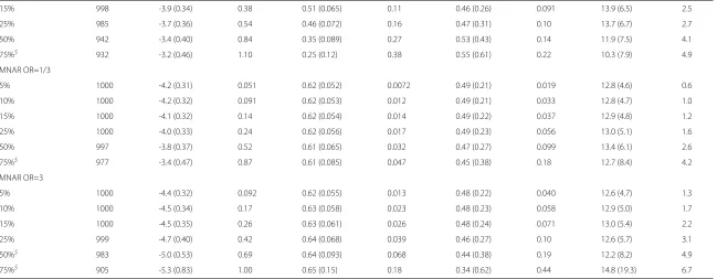
Table 2 Summary of parameter estimates obtained after multiple imputation of simulated missing data

Data1 _{N Intercept (SD) RMeSE}2 _Covariate3_{(SD) RMeSE}2 _σ2_{(SD) RMeSE}2 _Range4_{(SD) RMeSE}1 MCAR

5% 998 -4.3 (0.32) 0.046 0.62 (0.053) 0.0095 0.49 (0.22) 0.031 13.2 (5.3) 1.0

10% 998 -4.3 (0.33) 0.071 0.62 (0.055) 0.015 0.49 (0.23) 0.042 13.4 (5.5) 1.4

15% 998 -4.3 (0.33) 0.090 0.62 (0.057) 0.019 0.48 (0.23) 0.055 13.3 (5.8) 1.6

25% 997 -4.3 (0.35) 0.12 0.63 (0.060) 0.025 0.46 (0.24) 0.077 13.2 (6.0) 2.1

50%5 924 -4.3 (0.38) 0.22 0.62 (0.066) 0.042 0.40 (0.28) 0.13 15.1 (9.2) 3.6

75%5 571 -4.2 (0.39) 0.37 0.62 (0.069) 0.069 0.44 (0.38) 0.18 15.2 (15.0) 4.2

MAR0 OR=1/3

5% 1000 -4.3 (0.32) 0.054 0.62 (0.053) 0.012 0.49 (0.22) 0.038 13.4 (5.4) 1.3

10% 1000 -4.3 (0.33) 0.091 0.64 (0.056) 0.021 0.47 (0.22) 0.047 13.1 (5.4) 1.3

15% 1000 -4.3 (0.33) 0.10 0.64 (0.057) 0.022 0.46 (0.23) 0.058 13.1 (5.6) 1.5

25% 1000 -4.3 (0.35) 0.13 0.64 (0.060) 0.026 0.46 (0.24) 0.064 13.9 (6.4) 2.4

50%5 _{990 -4.3 (0.37) 0.20 0.65 (0.064) 0.041 0.42 (0.25) 0.10 14.1 (7.4) 2.7}

75%5 _{846 -4.3 (0.39) 0.31 0.65 (0.068) 0.060 0.41 (0.30) 0.14 15.0 (9.9) 3.6}

MAR0 OR=3

5% 1000 -4.1 (0.33) 0.17 0.58 (0.056) 0.047 0.46 (0.24) 0.067 14.7 (6.7) 2.3

10% 1000 -4.2 (0.33) 0.084 0.61 (0.056) 0.018 0.47 (0.23) 0.051 13.5 (5.9) 1.6

15% 1000 -4.3 (0.33) 0.10 0.62 (0.057) 0.021 0.46 (0.25) 0.076 13.4 (6.2) 1.5

25% 986 -4.2 (0.34) 0.13 0.61 (0.059) 0.027 0.41 (0.27) 0.11 14.5 (7.3) 2.7

50%5 821 -4.0 (0.35) 0.25 0.58 (0.063) 0.047 0.36 (0.29) 0.15 14.9 (11.0) 3.8

75%5 536 -4.0 (0.37) 0.32 0.58 (0.067) 0.069 0.44 (0.52) 0.19 16.1 (20.3) 4.6

MAR1 OR=1/3

5% 1000 -4.8 (0.34) 0.48 0.72 (0.059) 0.096 0.50 (0.23) 0.033 12.6 (5.0) 1.1

10% 1000 -4.9 (0.38) 0.61 0.75 (0.065) 0.12 0.51 (0.24) 0.041 12.4 (5.1) 1.2

15% 1000 -5.1 (0.38) 0.85 0.79 (0.066) 0.17 0.52 (0.25) 0.052 12.1 (5.0) 1.5

25% 1000 -5.4 (0.40) 1.08 0.84 (0.071) 0.22 0.53 (0.26) 0.060 11.2 (4.7) 1.9

50%5 _{1000 -5.6 (0.45) 1.30 0.88 (0.080) 0.26 0.54 (0.29) 0.081 10.5 (4.6) 2.5}

75%5 _{995 -5.8 (0.51) 1.52 0.93 (0.090) 0.30 0.52 (0.32) 0.093 10.5 (5.2) 2.8}

MAR1 OR=3

5% 1000 -4.1 (0.33) 0.17 0.57 (0.055) 0.051 0.46 (0.24) 0.069 14.5 (6.7) 2.4

10% 990 -4.0 (0.33) 0.28 0.54 (0.057) 0.079 0.43 (0.25) 0.087 15.4 (8.0) 2.9

Bihrmann

and

E

rsbøll

International

Journal

o

fH

ealth

G

eographics

2015,

14

:1

Page

6

o

f

1

3

http://www.ij-healthgeographics.com/content/14/1/1

Table 2 Summary of parameter estimates obtained after multiple imputation of simulated missing data(Continued)

25% 880 -3.7 (0.34) 0.54 0.45 (0.058) 0.17 0.44 (0.30) 0.10 14.6 (8.0) 2.8

50%5 _{644 -3.4 (0.34) 0.85 0.36 (0.059) 0.26 0.46 (0.35) 0.14 15.7 (11.2) 3.7}

75%5 _{566 -3.1 (0.33) 1.18 0.25 (0.062) 0.37 0.57 (0.50) 0.16 13.6 (12.6) 3.6}

MNAR OR=1/3

5% 1000 -4.2 (0.31) 0.064 0.62 (0.052) 0.0087 0.49 (0.22) 0.026 13.2 (5.3) 0.9

10% 1000 -4.2 (0.32) 0.092 0.62 (0.053) 0.011 0.49 (0.22) 0.038 13.3 (5.3) 1.2

15% 1000 -4.1 (0.32) 0.17 0.62 (0.054) 0.015 0.48 (0.22) 0.045 13.4 (5.6) 1.4

25% 1000 -4.1 (0.33) 0.22 0.62 (0.056) 0.018 0.46 (0.23) 0.064 13.7 (6.0) 1.8

50%5 972 -3.7 (0.33) 0.62 0.60 (0.057) 0.033 0.40 (0.23) 0.12 14.7 (7.3) 2.8

75%5 _{727 -3.3 (0.34) 0.98 0.59 (0.061) 0.051 0.34 (0.24) 0.18 15.4 (10.1) 3.9}

MNAR OR=3

5% 1000 -4.4 (0.32) 0.097 0.63 (0.055) 0.014 0.47 (0.22) 0.045 13.0 (5.3) 1.3

10% 1000 -4.5 (0.34) 0.18 0.63 (0.056) 0.023 0.49 (0.24) 0.057 13.6 (5.9) 1.8

15% 1000 -4.5 (0.40) 0.26 0.63 (0.061) 0.028 0.47 (0.25) 0.074 13.6 (6.3) 2.3

25% 983 -4.7 (0.40) 0.39 0.64 (0.067) 0.040 0.45 (0.29) 0.11 13.3 (7.0) 3.0

50%5 _{727 -5.0 (0.45) 0.46 0.64 (0.080) 0.046 0.50 (0.46) 0.14 13.9 (11.8) 3.6}

75%5 _{485 -5.3 (0.55) 0.98 0.63 (0.096) 0.10 1.16 (5.5) 0.67 15.9 (27.3) 4.5}

1_{Simulation scenarios described in the Methods section.}

2_{Square root of the median of (est. incomplete data - est. complete data)}2_. 3_{log(Herd size).}

4_{Range of influence in km.}

5_{Precision of prior distribution of hyperpar. changed from 0.001 to 0.1.}

Bihrmann and ErsbøllInternational Journal of Health Geographics2015,14:1 Page 7 of 13 http://www.ij-healthgeographics.com/content/14/1/1

The variance parameter estimates were all reasonably similar, but with a slight tendency to either increase (espe-cially MAR0 OR=1/3 and MAR1 OR=1/3) or decrease (especially MAR0 OR=3) with more than 50% missing data. Both the standard deviation of each parameter estimate, and the Root Median Squared Error (RMeSE) increased when the number of missing observations was increased, regardless of scenario.

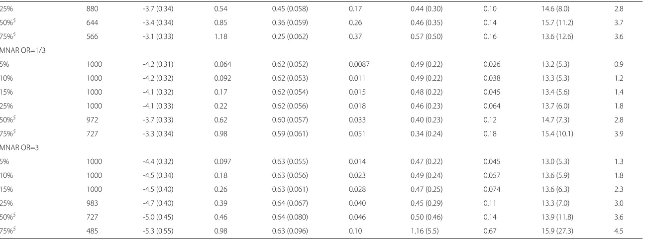
The median of the estimated range of influence within each simulation scenario (Figure 1) ranged from 9.4 km (SD 4.0) (MAR1 OR=1/3, 75%) to 14.8 km (SD 19.3) (MNAR OR=3, 75%). In all scenarios except MAR1, the range estimates were quite similar with less than 50% missing observations. They tended to be slightly larger than the estimate obtained from the complete data, but differences were small, especially taking into account the uncertainty of the estimates. With≥ 50% missing obser-vations, the variation between scenarios increased, yet so did the standard deviation of each estimate. There was no strict pattern relating to the number of missing obser-vations displayed, except in the MAR1 OR=1/3 scenario where the range decreased with increasing number of missing observations.

Overall, the most pronounced effect on the range esti-mate was seen in the MAR1 scenarios, where the missing observations were dependent upon the covariate. The spe-cific effect of missing data on the range estimate in these scenarios is the result of the combination of the covariate and the outcome, as well as their spatial distribution, and

Figure 1Range of influence in missing data.Estimated range of influence in complete data (solid line) and simulated missing data. Simulation scenarios were: A: MCAR, B: MAR0 OR=1/3, C: MAR0 OR=3, D: MAR1 OR=1/3, E: MAR1 OR=3, F: MNAR OR=1/3, G: MNAR OR=3.

the effect might therefore be different in another data set. The range of influence might also actually depend on the covariate, yet a potential explanation for the observed pat-tern is not obvious. In the MAR0 scenarios, the missing observations were directly related to the spatial structure of the data, and a more distinct effect than the observed might have been expected.

No detectable spatial correlation (range ≥ 75 km) occurred mainly among data sets with 50% and/or 75% missing observations. This is where we would expect that any spatial correlation would be most depleted by the missing data. This happened in a maximum of 95 of 1000 data sets, which was in the MNAR OR=3, 75%-scenario, where observations with a positive outcome status were most likely to be missing and hence only very reduced information about model parameters were con-tained in the data. The MAR1 OR=1/3 scenario was the only scenario where all data sets displayed a spatial cor-relation, even with 75% missing data. The MAR1 OR=3 scenario, on the contrary, had more data sets displaying no spatial correlation than any other scenario. This could partly be explained by the changed prevalence in the data (increased prevalence in the MAR1 OR=1/3 scenario and vice versa), but the pattern was not as pronounced when the missing data depended on the outcome itself (MNAR scenarios). This suggests that the observations excluded in the MAR1 OR=3 scenario exhibited the strongest spa-tial correlation. This would again be related to the specific data set.

The RMeSE of the range increased with an increas-ing number of missincreas-ing observations in all scenarios. The increase was especially pronounced with more than 50% missing data. Hence, even though the overall median of the range estimates did not change much, more sub-stantial deviations from the estimate obtained from the complete data did occur within single data sets with more than 50% missing data. In the MCAR 75% scenario, for example, the median range was 0.2 km larger than in the complete data, but the median deviation was 5.4 km.

Imputed data

Multiple imputation did not remove the bias of the regres-sion parameter estimates introduced by the missing obser-vations (Table 2). This was as expected, since only the outcome was missing. In that case, it is well-known that imputation will not remedy any bias of regression param-eter estimates, e.g. von Hippel [5].

Bihrmann and ErsbøllInternational Journal of Health Geographics2015,14:1 Page 8 of 13 http://www.ij-healthgeographics.com/content/14/1/1

Figure 2Range of influence in multiple imputed data.Estimated range of influence in complete data (solid line) and after multiple imputation of simulated missing data. Simulation scenarios were: A: MCAR, B: MAR0 OR=1/3, C: MAR0 OR=3, D: MAR1 OR=1/3, E: MAR1 OR=3, F: MNAR OR=1/3, G: MNAR OR=3.

deviation of each range estimate increased after multiple imputation. With multiple imputation of less than 50% missing observations, the RMeSE tended to be slightly larger than the results obtained from the missing data. With multiple imputation of≥50% missing observations, the RMeSE was slightly smaller. Therefore, considering estimation of the range of influence, at least 50% miss-ing observations were required to potentially benefit from multiple imputation, and this was at the expense of an increased standard deviation. It should be noted, however, that the results with imputation of≥50% missing obser-vations were based on the informative prior distribution, which in case of missing data was only used with 75% missing observations.

The number of data sets (N) with detectable spatial cor-relation in Table 2, was not directly comparable to the corresponding number in Table 1. In multiple imputation, the incomplete data set is substituted by a set of complete data sets. If any of the data sets in such a set did not exhibit spatial correlation (i.e. the range estimate was≥75 km), then the whole set was excluded from Table 2. This was done in order to retain the number of imputations in each incomplete data set. For example, 429 sets of imputed data were excluded in the MCAR 75% scenario. This means that at least 429 of 10000 imputed data sets (10 for each incomplete data set) showed no detectable spatial corre-lation, as compared to 60 of 1000 incomplete data sets. In this scenario actually 970 of 10000 imputed data sets

showed no spatial correlation. Overall, a lack of spatial correlation occurred more frequently with imputed data than with missing data (data not shown), and mainly with imputation of more than 50% missing observations.

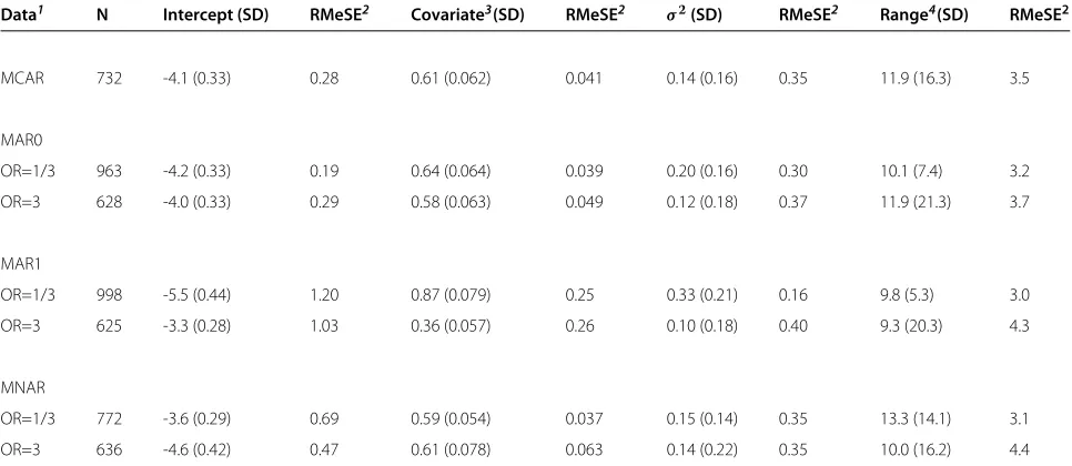
The parameter estimates obtained after multiple impu-tation without a spatial component were summarised in Table 3. Only results with imputation of 50% missing data were shown. The regression parameter results were similar to the results obtained with multiple imputation based on the spatial model. In all scenarios, the variance parameter estimate was much smaller when not including the spatial component in the imputation. The estimated range of influence also tended to be smaller, but the stan-dard deviation of the estimate was considerable in most scenarios. Compared to imputation based on the spatial model, more data sets showed a lack of spatial correlation. This was expected, since the imputed data had no spatial structure.

Conclusion

This simulation study investigated how the estimated range of influence was affected by missing outcomes in binary spatial data. This is a relevant topic since miss-ing data are a common feature in many analyses. The results showed that the effect on the range estimate was to some extent dependent upon the missing data mech-anism. When the missing outcomes were MCAR, MAR depending on a covariate not correlated with the outcome, or even MNAR, the range estimates were consistent with ≤ 25% missing data. When the missing outcomes were MAR depending on a covariate which correlated with the outcome, the range estimate was affected by even a moderate number of missing observations. In this specific study, however, the considered covariate was possibly also related to the range itself. This added to the complexity of the situation and may have also contributed to the effect of the missing outcomes in this scenario. In general, the over-all effect of missing observations was smover-all compared to the uncertainty of the range estimate. Multiple imputation of the missing observations provided a potential improve-ment in the range estimate in the case of≥50% missing data, but with increased uncertainty of the estimate as a consequence.

Bihrmann and ErsbøllInternational Journal of Health Geographics2015,14:1 Page 9 of 13 http://www.ij-healthgeographics.com/content/14/1/1

Table 3 Summary of parameter estimates obtained after multiple imputation of 50% simulated missing data

Data1 _{N Intercept (SD) RMeSE}2 _Covariate3_{(SD) RMeSE}2 _σ2_{(SD) RMeSE}2 _Range4_{(SD) RMeSE}2

MCAR 732 -4.1 (0.33) 0.28 0.61 (0.062) 0.041 0.14 (0.16) 0.35 11.9 (16.3) 3.5

MAR0

OR=1/3 963 -4.2 (0.33) 0.19 0.64 (0.064) 0.039 0.20 (0.16) 0.30 10.1 (7.4) 3.2

OR=3 628 -4.0 (0.33) 0.29 0.58 (0.063) 0.049 0.12 (0.18) 0.37 11.9 (21.3) 3.7

MAR1

OR=1/3 998 -5.5 (0.44) 1.20 0.87 (0.079) 0.25 0.33 (0.21) 0.16 9.8 (5.3) 3.0

OR=3 625 -3.3 (0.28) 1.03 0.36 (0.057) 0.26 0.10 (0.18) 0.40 9.3 (20.3) 4.3

MNAR

OR=1/3 772 -3.6 (0.29) 0.69 0.59 (0.054) 0.037 0.15 (0.14) 0.35 13.3 (14.1) 3.1

OR=3 636 -4.6 (0.42) 0.47 0.61 (0.078) 0.063 0.14 (0.22) 0.35 10.0 (16.2) 4.4

1_{Simulation scenarios described in the Methods section}2_{Square root of the median of (est. incomplete data - est. complete data)}23_{log(Herd size)}4_{Range of influence}

in km. Imputation was based on a standard logistic regression model without inclusion of a spatial component. All results are medians of N data sets.

and could potentially provide a better solution, especially when working with a specific data set as opposed to the automated analyses of a simulation study.

This study was based on the simulation of missing data in a specific complete data set. The “true” range of influence was defined by this complete data set and was not varied within the simulations. To fully explore a possible dependence on for example the extent of the range and the strength of the correlation, would require completely simulated data sets. This should include the spatial locations of the observations, since different spa-tial patterns may also influence the effect of missing observations.

Methods

Data

The study was based on a complete data set with simu-lated missing outcome. All information (outcome, covari-ates, and locations) was taken from the complete data set, and then some of the observations were defined to be missing, according to different simulation sce-narios. Data on Salmonella Dublin in Danish cattle herds were used as the complete data set. These data were available, since Denmark has a mandatory surveil-lance program on Salmonella Dublin. The Salmonella Dublin infection as such was not of any interest in this study.

The complete data set included all Danish cattle herds from the beginning of 2003 to the end of 2009. For all herds, information from the Danish Cattle Database (hosted by Knowledge Centre for Agriculture, Aarhus N, Denmark) included unique herd ID number,

geographical coordinates in UTM-format, geographical region (Figure 3a), herd size (total number of cattle), Salmonella Dublin ELISA measurements on bulk-tank milk or blood samples, and date of bulk-tank milk or blood sampling. Based on this, the number of herds per km2 within a 5 km radius of each herd was calculated (herd density), and all herds had aSalmonella Dublin classifi-cation status (positive/negative) assigned for each quarter of the year. For details on the definition of herd infection status, please refer to [6].

For the analysis, all cattle herds located in the south-ern part of Northsouth-ern Jutland (region NJS) (Figure 3a) in the last quarter of 2008 were included (N=1597). Four herds had no information on herd size (assumed miss-ing completely at random). Since the focus in this study is on missing outcomes, these herds were excluded; result-ing in a total of N=1593 (470 dairy, 1123 non-dairy) herds. Among these, 278 herds (17.4%) had a positiveSalmonella Dublin status (Figure 3b). The considered covariates were herd size (Figure 3c) and herd density (Figure 3d). Herd size was log-transformed since the distribution was skewed. Herd size correlated with Salmonella Dublin status (corr=0.35, p<0.0001), whereas herd density and Salmonella Dublin status did not significantly correlate (corr.=0.044, p=0.082). Herd size and herd density were uncorrelated (corr=0.035, p=0.17).

Simulation of missing outcome

Bihrmann and ErsbøllInternational Journal of Health Geographics2015,14:1 Page 10 of 13 http://www.ij-healthgeographics.com/content/14/1/1

Figure 3Descriptive maps.Denmark divided into 8 geographic regions(a), including NJS (southern part of Northern Jutland) withSalmonella

Dublin status of all cattle herds(b), total number of cattle within herds(c), and number of herds within a 5 km radius(d).

(Mi)i=1,...,1593withMi ∈ {0, 1},i = 1,. . ., 1593. IfMi = 1, the corresponding observation yi was set to missing. Scenarios with 5%, 10%, 15%, 25%, 50%, and 75% miss-ing observations were considered. Within each scenario, 1000 replications ofMwere produced. Through the sim-ulation of M, observations within y were defined to be missing in three different ways: 1) missing completely at random (MCAR), 2) depending on an observed covari-ate (MAR), and 3) depending on the observation itself (MNAR).

Each vector M = (Mi)i=1,...,1593 was generated by drawing from independent Bernoulli distributions with parameterπi(= probability of being missing). To produce

observations missing completely at random,πiwas given by

logit(πi)=μ, i=1,. . ., 1593, (1)

whereμwas chosen corresponding to the proportion of missing data in each scenario. To produce missing obser-vations depending on a completely observed covariate

X=(Xi)i=1,...,1593,πiwas given by

logit(πi)=μ+ν·

Xi−X

, i=1,. . ., 1593, (2)

Bihrmann and ErsbøllInternational Journal of Health Geographics2015,14:1 Page 11 of 13 http://www.ij-healthgeographics.com/content/14/1/1

(referred to as the MAR1 scenario), whereas herd density did not correlate with the outcomey(referred to as the MAR0 scenario). The parameterμwas chosen as above, and two values of ν were considered: corresponding to OR=1/3 and OR=3 of being missing when increasing the covariate one unit. Missing observations depending on the outcome y = (yi)i=1,...,1593 were produced by letting

logit(πi)=μ+ν·(yi−y), i=1,. . ., 1593, (3)

with parametersμ,νchosen as above.

Statistical model

Letyidenote the binary outcome (0/1) at locationzi,i= 1,. . .,N. Withpi = P(Yi=1),i = 1,. . .N, the logistic regression model is given by

logit(pi)=α+βXi+U(zi), i=1,. . .,N, (4)

where Xi is a covariate (vector) with corresponding parameter (vector) β, and U(zi) is a realisation of a latent stationary Gaussian field (GF) representing the spatial dependence between observations. Hence, U =

(U(zi))i=1,...,Nhas a multivariate normal distribution with spatially structured covariance matrix . The (r,s) ele-ment of is given by the Matérn spatial covariance function

σ2

2λ−1_(λ)(κ rs) λ_K

λ(κ rs), (5)

where rs denotes the distance between locationzr and zs, andKλ is the modified Bessel function of the second kind and order λ. The smoothness parameterλ is typi-cally poorly identified and was fixed at 1, κ is a scaling parameter, andσ2_{is the marginal variance. This} covari-ance function was verified as providing a suitable model for the data by fitting it to the sample semivariogram of the residuals obtained from fitting the logistic regression (4) without the GF. Based on the covariance function (5), the range of influence is defined as√8λ/κ, as in [1]. This cor-responds to the distance at which the spatial correlation is close to 0.1 for allλ.

Inference about model parameters was based on the Stochastic Partial Differential Equation (SPDE) approach proposed by [1]. This approach uses a linear combina-tion of basis funccombina-tions defined on a triangulacombina-tion of the spatial region to represent the GF by a Gaussian Markov random field (GMRF). Given a triangulation withV ver-tices located at (z˜v)v=1,...,V and a set of basis functions

(ψv)v=1,...,V (each chosen to be piecewise linear withψv= 1 atz˜vand 0 at all other vertices) the GF is represented by

U(z)= V

v=1

ψv(z)U(z˜v), for allz, (6)

where U = Uz˜v

v=1,...,V is a GMRF with precision matrixQκ,σ2depending on the parametersκandσ2in (5) (sinceλis fixed at 1). Now model (4) can be rewritten as

logit(pi)=α+βXi+ V

v=1

Aiv(zi)U

˜ zv

, (7)

where the matrixA = (Aiv(zi))i=1,...,N,v=1,...,V is the pro-jection from the triangulation vertices to the observation locations (which are not necessarily included as vertices).

Inference

Based on a triangulation of the spatial region and the model specified in (7), parameters were estimated using the Integrated Nested Laplace Approximation (INLA) approach proposed by [2]. This approach to Bayesian inference provides deterministic approxima-tions to the posterior marginals for all parameters and is based on Laplace approximations [7]. Computations were done in R version 3.0.2 [8] using the INLA pack-age (www.r-inla.org), which includes the SPDE approach as a standard method. The regression parameters α, β were assigned independent, normal prior distributions with precision 0.001, andUwas assigned the GMRF with precision Qκ,σ2as described above. The variance σ2 was parametrised asσ2 = 1/2πκ2τ2, and the hyper-parameters (log(κ), log(τ)) were assigned normal prior distributions with known precision. Sensitivity analysis to assess the effect of the prior distribution was carried out by considering three values of this precision: 0.1 (the default of the INLA package), 0.001, and 0.00001.

The INLA package also provides a function for produc-ing the required triangulation of the spatial region. The triangulation of the spatial region is shown in Figure 4. All 1593 locations were included as vertices, and additional vertices were added to produce a regular mesh. The mesh extends beyond the border of the considered region to correct for edge effects. The maximum allowed triangle edge length was 2 km inside the region and 50 km outside the region. The minimum allowed distance between ver-tices was 0.75 km. The triangulation consisted of a total of 2248 vertices.

Bihrmann and ErsbøllInternational Journal of Health Geographics2015,14:1 Page 12 of 13 http://www.ij-healthgeographics.com/content/14/1/1

Figure 4Triangulation of the spatial region.The mesh extends beyond the border of the considered region to correct for edge effects. The maximum allowed triangle edge length was 2 km inside the region and 50 km outside the region. The minimum allowed distance between vertices was 0.75 km. The triangulation consisted of a total of 2248 vertices.

with complete data - estimate with missing data)2_within each simulation scenario.

The simulated data were analysed using parallel com-puting. Analyses were run on an external supercomputing facility (i.e. a cluster of computers), due to the size of the simulation study. Parallel computing could, however, be performed on any standard personal computer with multiple CPU cores. Parallel computing is very useful for simultaneous analysis of multiple data sets, for example in simulation studies or with multiple imputed data. It cannot be used when analysing a single data set.

Parallel computing was performed using the R package parallel. With the chosen triangulation and the required output (e.g. predicted values) it took around 12-15 hours to analyse 1000 data sets (16 cores, 2.66Ghz CPU). R code is supplied as Additional file 1.

Multiple imputation

Imputation of the simulated missing outcome was based on model (7), which was fitted to the available data. The available covariates (herd density and (log-) herd size) were included in the model. A predicted probability was sampled from the posterior distribution, and a binary out-come was then generated based on this probability. This was done at each location where the outcome was not observed, whereby a complete data set was created. This process was repeated to produce a number of imputed

data sets corresponding to each incomplete data set. The number of imputed data sets created depended on the amount of missing observations. This was done in an attempt to ensure the same efficiency of the estimates across the simulation scenarios. Classical recommenda-tions [4] suggest that only a small number of imputed data sets are needed, hence 3 data sets were created when 5% of data were missing, 5 data sets were created when 10%, 15%, 25% of data were missing, and 10 data sets were cre-ated when 50%, 75% of data were missing. Each imputed data set was analysed individually, and estimates were then combined using Rubin’s rules [3] to obtain the overall estimates corresponding to each incomplete data set. In general, each individual estimate should be approximately Gaussian distributed and otherwise transformed prior to combination [9]. The estimates of the variance parameter σ2_{and the range of influence had skewed distributions,} and were therefore log-transformed. The combined esti-mate on the original scale was subsequently obtained using standard theory for the lognormal distribution [10]. Hence, if θ˜m is the individual estimate obtained as the mean value of the log-transformed posterior distribution, andθ˜ is the combined estimate obtained fromθ˜m, m = 1,. . .,M, then the combined estimate on the original scale is given by

Bihrmann and ErsbøllInternational Journal of Health Geographics2015,14:1 Page 13 of 13 http://www.ij-healthgeographics.com/content/14/1/1

where ω2 _{= Varθ}˜_{. The variance of the combined} estimate on the original scale is given by

exp2θ˜+ω2_{/2 expω}2_−1.

For comparison, the imputation model was changed from model (7) to a standard logistic regression model without inclusion of a spatial component.

Additional file

Additional file 1: R code for analysis using the INLA package and parallel computing.

Competing interests

The authors declare that they have no competing interests.

Authors’ contributions

KB carried out the analyses and drafted the manuscript. AKE participated in the design of the study and revised the manuscript. Both authors read and approved the final manuscript.

Acknowledgments

KB was funded by a PhD grant at the Faculty of Health and Medical Sciences, University of Copenhagen. The authors would like to thank Søren Saxmose Nielsen for revising the manuscript, and Nils Toft for commenting on analyses and revising the manuscript.

Author details

1_{Faculty of Medical and Health Sciences, University of Copenhagen,}

Grønnegårdsvej 8, DK-1870 Frederiksberg C, Denmark.2National Institute of Public Health, University of Southern Denmark, Øster Farimagsgade 5A, 2, DK-1353 Copenhagen K, Denmark.

Received: 10 October 2014 Accepted: 16 December 2014 Published: 6 January 2015

References

1. Lindgren F, Rue H, Lindström J. An explicit link between Gaussian fields and Gaussian Markov random fields: the stochastic partial differentation approach. J R Stat Soc B 2011;73 Part 4:423–498.

2. Rue H, Martino S, Chopin N. Approximate Bayesian inference for latent Gaussian models by using integrated nested Laplace approximations (with discussion). J R Stat Soc B 2009;71(2):319–392.

3. Little RJA, Rubin DB. Statistical analysis with missing data, 2nd ed. Hoboken, New Jersey: Wiley; 2002.

4. Rubin DB. Multiple imputation for nonresponse in surveys. New York: Wiley; 1987.

5. von Hippel PT. Regression with missing ys: An improved strategy for analyzing multiply imputed data. Sociol Methodol 2007;37:83–117. 6. Ersbøll AK, Nielsen LR. The range of influence between cattle herds is of

importance for the local spread ofSalmonellaDublin in Denmark. Prev Vet Med 2008;84:277–290.

7. Tierney L, Kadane J. Accurate approximations for posterior moments and marginal densities. J Am Stat Assoc 1986;393(81):82–86.

8. R Core Team. R: A language and environment for statistical computing. Vienna, Austria: R Foundation for Statistical Computing; 2013. http://www.R-project.org/

9. White IR, Royston P, Wood AM. Multiple imputation using chained equations: Issues and guidance for practice. Stat Med 2011;30:377–399. 10. Aitchison A, Brown JAC. The Lognormal Distribution. London: Cambridge

University Press; 1957.

doi:10.1186/1476-072X-14-1

Cite this article as:Bihrmann and Ersbøll:Estimating range of influence in case of missing spatial data: a simulation study on binary data.

International Journal of Health Geographics201514:1.

Submit your next manuscript to BioMed Central and take full advantage of:

• Convenient online submission

• Thorough peer review

• No space constraints or color figure charges

• Immediate publication on acceptance

• Inclusion in PubMed, CAS, Scopus and Google Scholar

• Research which is freely available for redistribution