Unilateral Commitments

(1)

UNIVERSITY of TRENTO

Department of Mathematics

Doctorate in Mathematics

20

th

course

PhD Thesis

Unilateral Commitments

Supervisor Phd Student

prof.Fioravante Patrone Federica Briata

(2)

(3)

Introduction

Game Theory is a mathematical theory which deals with conflict and coo-peration situations between (at least two) intelligent and rational decision-makers and provides mathematical models of them. The subjects of study for game theorists are not merely play activities as the term “ game” erro-neously suggests. “Conflict analysis” or “interactive decision theory ” might be names more suitable to describe this theory.

A conflict or cooperation situation (game) is a strategic interaction bet-ween two 1 or more individuals (players), which jointly determine the out-come. Each player partially controls the game, but usually no player has full control.

It is convenient to be more precise about the assumptions of intelligence and rationality. With the first hypothesis, we assume that the decision mak-ers have unlimited capacities of deduction, computation, and analysis of the situation. With the second hypothesis, we assume that the decision maker is able to make a choice between various available options. The rationality of the decision maker lies in having preferences on the consequences of his choice, in the consistency with these preferences, and in choosing the avail-able action whose consequence he prefers. The keyword “rationality” is a term inherited from Neoclassic Economics and Decision Theory from which Game Theory derives.

A game is not only made up of players and of choices available to the players, but also of preferences of the players over the set of possible out-comes of the games. Thus, each player strives to obtain the most profitable outcome for him. Often it is assumed that these preferences are described by a von Neumann-Morgenstern utility function, hence with each player there is associated a numerical function whose expected value he tries to maximize.

1

The case of one player usually falls under the heading of “Decision Theory”.

(4)

So Game Theory is not only an empiric theory, but also a normative theory, since it prescribes what action each player should choose in a game in order to promote his interests optimally, that is, which strategy each player should play to obtain the best benefits with only his partial influence on the situation.

The aim of Game Theory, as stated in Von Neumann and Morgenstern (1944), is to find the mathematically complete and perfectly general princi-ples which define “rational behavior” for the players in a game and to derive from them the characteristics of that behavior. While the principles ought to be perfectly general, that is, valid in all situations, the solution can be found only in some special characteristic cases and it varies with the change of conditions.

Game Theory is a relatively recent science. Its beginnig dates back to the 20th century with the works of Zermelo (1913), Borel (1921), von Neumann (1928) 2. But the theory was considered only after the publication of the book by von Neumann and Morgenstern (1944), followed by many articles addressed to developments of this theory. We remember, for example, John F.Nash Jr. (1950), in which the author introduced the Equilibria-bargaining threat.

Many studies of Game Theory were completed during World War II at Princeton, in the same cultural circle where many theoretical physicists were also working (see Morgenstern (1976)). According to the opinion of Myerson (1991), this propinquity does not seem coincidental, however the purpose of the two groups proved different. The physicists have developed the nuclear studies which have threatened the world peace, the game theo-rists have created social systems for moderating human behavior in conflict. Thus, it might be desiderable that the improvements of social systems were able to study the situation and to outguess the consequences of the physical science. This convinction has moved mathematicians and social scientists to work in Game Theory during the past few years, although there is lack of collaboration between the various disciplines. For example, the production of bio-diesel, extracted from sunflower oil or colza oil, has been a positive en-vironmental impact, but it has created problems of famine to poor countries whose economy was based on primary sectors.

Game Theory actually has proved to be versatile since used in many fields. It has been applied in Military Strategies (Cold War, Gulf War), in Economics (Oligopolies, Monopolies), in Marketing (Coca-Cola), in Finance

2

(5)

Unilateral Commitments iii

(Firm’s Control), in Politics (Electoral Systems), in Club Games (Bridge, Poker, Chess), in Sports (Attack-Defence Strategies), in Sociology (Migra-tion), in Medicine (Neurons), Genetics/Biomedicine (Microarray Games), in Psychology (Prisoner’s Dilemma), in Biology (Evolution), in Environment (Pollution).

The importance of developments achieved in Game Theory is supported and affirmed by the assignment of Nobel prizes in Economics. In fact, re-cently, eight game theorists shared the Nobel prize in economics. They were: in 1994 John F.Nash Jr., John Harsanyi, and Reinhard Selten; in 2005 Y.Robert J. Aumann and Thomas C. Schelling; in 2007 Roger My-erson, Leonid Hurwicz, and Eric Maskin. Nash defined the notion of a noncooperative (or Nash) equilibrium, and proved its existence in mixed strategies. Selten refined this notion to the recursive notion of subgame per-fect equilibrium and the closely related notion of trembling hand perper-fection. Harsanyi defined the notions of a game with incomplete information and of a Bayesian equilibrium, in which players’ lack of information about the game they are playing is encapsulated in a player’s ”type.” These ideas have been influential in the study of games by economists during the 1980s. Four major areas in which this impact has been felt are in the study of bargaining, reputation and repeated games, signalling, and mechanism design.

Traditionally, the mathematical models of strategic interactions are di-vided into two classes: cooperative games and non-cooperative games. A cooperative game is a game in which the players can subscribe binding agree-ments. A non-cooperative game is one in which there are no possibilities for communication, correlation or (pre)commitment, except for those that are explicitly allowed by the game rules. Hence, all relevant aspects should be captured by the rules of the game. In this work, we restrict ourselves to noncooperative games.

(6)

The concept of Nash equilibrium is a concept relevant and increased in value solution, not only for the idea of stability of non-binding agreements, but also since it plays on the assumptions of intelligence and rationality of players and it does not request the players to communicate to each other before strategic interaction. However, it has its drawbacks. Given a game, various problems can arise, from problems of existence of equilibria to pro-blems of choice of an equilibrium that brings to an efficient outcome. For example, a game so simple as Matching Pennies is without Nash equilibria. Otherwise, we might have two or more possible choices for the players: the Coordination game has two Nash equilibria with the same payoffs, while the Battle of the Sexes has two Nash equilibria, each of them is preferred only by one player. Or, again, there are games with inefficient Nash equilibria, as it happens for Prisoner’s Dilemma.

The intervention of Game Theory lies in providing the players with dif-ferent kinds of solutions of the game. For example the study of refine-ments of Nash equilibria is one of the knottiest problems in Game Theory. Among the proposed refinements, we can mention trembling hand perfect equilibrium (Selten (1975)), proper equilibrium (Myerson (1978)), sequential equilibrium (Kreps and Wilson (1982)), stable equilibrium (Kohlberg and Mertens (1986)), and virtual subgame perfect equilibrium (Garc´ıa-Jurado and Gonz´alez-D´ıaz (2006)).

(7)

Unilateral Commitments v

lead to cooperative equilibria. In the example of the Tragedy of the Com-mons, despite the pessimistic theoretical predictions about cooperation, a lot of partial agreements are signed by a subset of countries trading. Thus, it emerged that man is a social being, which spontaneously cooperates. But the cooperation is partial, not global. The final goal becomes to find how the global cooperation is reached.

Again, let us consider the case of public goods. If a public good is local, then in order to conserve it from over-exploitation a local authority is sufficient. But in case of international public goods, this is not possible, then there are international negotiations and contracts signed by a part the of countries interested in cooperation. Comparing the theoretical results with concrete facts, there is a paradox. That is, there is not always the over-exploitation of public good, as predicted by theory. In fact, more than 120 international environmental agreements are signed. At this point, the game theory intervenes in order to emerge cooperation between all the countries or among a greater and greater number of individuals. The environment is, for example, one of the international public goods. In the global environmental problems a target to reach is the reduction of greenhouse gas emissions. All the countries are actively and passively concerned in this problem, in fact they regulate the threshold of their own gas emissions and they suffer the consequence also from the economic point of view of greenhouse effect: melt of glaciers and rising water level cause damage to agriproducts. World emergency requires an international coordination between countries aiming at signing agreements to reduce gas emissions, but, in practice, the signers are a small number. Even Game Theory confirms this behaviour. Carraro and Marchiori (2003), for example, show a model where, at the equilibrium, the signatories are fewer in number and the grand coalition is not achieved. We prove the same results in Section 3.6. The seriousness of the problem needs all the countries to sign agreements and reduce their gas emissions.

The Thesis consists of four parts: the first part contains opening notes, while the others refer to three different problems: the analysis of a binary symmetric game, a modified version of Unilateral Commitments Game, and the essentializing of different equilibrium concepts.

(8)

exten-sive form, and the coalitional form. First, we introduce games in strategic form, the dominated strategies , the concept of Nash equilibrium, and some games quoted in this work, such as Matching Pennies, Coordination Game, Battle of the Sexes, Prisoner’s Dilemma, and Rock Paper Scissors. Then, we present games in extensive form with perfect recall, followed by games in coalitional form and, in particular we recall the definition of T U IC-games, since the model analyzed in Chapter 3 derives from them. In the conclu-sive Section of Chapter 1, we present those refinements of Nash equilibria, which we have essentialized in Chapter 5 , not based on beliefs, like Sub-game Perfect Equilibrium (SPE), and Perfect Equilibrium (PE), and based on beliefs, like Sequential Rationality (SR), Sequential Equilibrium (SE), and Weak Perfect Bayesian Equilibrium (WPBE).

In Chapter 2, we present the concept of potential, and its relations with symmetric games. The Section 2.5 is the core of Chapter 2 and provides our results. The first result establishes a symmetric game with only two strategies is a potential game and then it has a pure Nash Equilibrium. The originality of the result lies in beying such a game a potential game, since Cheng and other (2004) has already showed that a symmetric game with only two strategies has a pure Nash equilibrium. The second one provides how all the NE of a symmetric, binary game are deduced from its potential function.

The second part of the Thesis is Chapter 3, where we present two models of binary games. We consider the problem of sharing the cost of facilities among the possible users. An easy way to divide costs is to divide them evenly among all of the players. But this way violates fairness, and, it would be reasonable to take into account whether a member uses or not a given facility. In order to be able to enforce the payment, we assume to have a way to make verifiable to a third part who are the users, but, to make it verifiable, an additional cost is to be added. We propose two ways, in which players reach such a decision. In the first model, the naming game, each player names the machine for which he asks for verifing. In the second model, the majority decision game, the checking is made only if the given quorum is reached. Each model has been examined first in the case with only one machine and then with different ones. Since a binary symmetric game is a potential game and, then, it has a pure Nash Equilibrium, we can model a special case of environmental game via naming game, that is via a potential or congestion game, result processed in Section 3.6.

(9)

Unilateral Commitments vii

stage, each player declares that he will pay a penalty if he will not play, in the second stage, the restricted strategies. Adding a self-punishing scheme to this simple sequential game structure makes self-enforcing the Nash equi-libria of the constituent game, if any. In particular, we embed a two player game into a two stage game, in which players can restrict their strategy spaces in the first stage. In the second stage, if player chooses a strategy from his restricted strategy space, he obtains the same payoff as in the ba-sic game, otherwise he pays a penalty dependent on the square of distance from his restricted strategy space. Since a commitment is a binding of an individual to the others, it measures an attitude to the sense of altruism, compliance, identification and loyalty towards the group. It is no accident we have called our model as quality commitments instead of penalty com-mitments. In this years, the Corporate Social Responsability (briefly, CSR) is developping. A CSR is an enterprise, which not only produces wealth, but also is dealing with business within the competence of State, Church, civil society, and family. In order to favour the cooperation in a game, usually we implement an efficient disciplinary system, extern to the parts involved in the game. Instead, the CSR develops on civic virtue: the virtue cannot be negotiated, like penalty is settled by contract, but it is a product of free will. The same it happens in our model of QUC, since the sanctions is self declared by the players, then it is internal to the game.

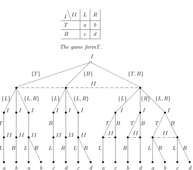
The fourth part of the Thesis (Chapter 5) is an annotated rewrite of the paper Essentializing Equilibrium Concepts, together with Gonz´alez-D´ıaz , Garc´ıa-Jurado, and Patrone (see Gonz´alez-D´ıaz et al. (2009)). The essen-tializing process is a tool to identify what information about a game may be neglected, in order to check whether a specific profile correspond to an equi-librium outcome or not. Given an extensive game, an equiequi-librium concept selects a set of strategy profiles (empty too) satisfying well-defined condi-tions testing on the all game tree We characterize the essential colleccondi-tions for the most used equilibrium concepts, based or not on beliefs, such as SR, WPBE, SE or NE, SPE, PE. The possible applications of our analysis is to check the robustness of a concept, to analize a partially-specified game, and, finally, to study the concept of Virtual Equilibrium.

(10)

(11)

Chapter 1

Preliminaries

In this Chapter we define the basic concepts of Game Theory, fundamental for this work, and set up standard terminology and notations. First, we introduce games in strategic form (Section 1.1), dominated strategies (Sub-section 1.1.2), the concept of Nash equilibrium (Sub(Sub-section 1.1.3), and some games quoted in this work (Subsection 1.1.4), then games in extensive form (Section 1.2), followed by games in coalitional form (Section 1.3, and, in particular we recall the definition of T U IC-games (Subsection 1.3.1), since we quote them in Chapter 3. In the conclusive Section 1.4, we present some refinements of Nash equilibria, not based on beliefs (Subsection 1.4.1), like Subgame Perfect Equilibrium (SPE), and Perfect Equilibrium (PE), and based on beliefs (Subsection 1.4.2), like Sequential Rationality (SR), Sequen-tial Equilibrium (SE), and Weak Perfect Bayesian Equilibrium (WPBE).

As we have reminded in the Introduction, Game Theory copes with strategic interaction between at least two decisioners, called players, and makes mathematical models of it. The players (or else sets of players), intelligent and rational, interact with each other in situations of conflict and cooperation. Each player masters partially the end result of the game

1 _{through his actions. This way, we have identified the constituents of a}

game.

Definition 1. A game G is composed of at least two players, the choices at disposal of players, and the preferences of players compared to game out-comes.

We assume that the players are rational and intelligent, and the model

1_{A game is made up of players (at least two), of choices at disposal of the players, and}

preferences of the players for outcomes of the games.

(16)

is common knowledge (Lewis (1969). We say rational the player able to make a choice between various available options, andintelligent the decision maker with unlimited capacities of deduction, calculus, and analysis of the situation. The structure of the game iscommon knowledge when we assume that all players know the structure of the strategic form, and know that their opponents know it, and know that their opponents know that they know, and so on ad infinitum.

The games are divided intocooperative games, if players can sign binding agreements, andnon-cooperative games, otherwise.

A game can be described in several ways, the principal forms are three: the strategic form, the extensive form, and the coalitional form. The first two classes belong to non cooperative games theory, the third class to coo-perative games theory. A game in strategic form is represented by listing all the strategies (complete plan of action) available to each player, together with the payoffs associated with the various strategy combinations. The strategic form, or s.f., is recomended for games with simultaneous and in-dependent actions. A game in extensive form is given by the rules of the game indicating the choices available to each player, the information of a player when it is his turn to move, and the payoffs each player receives at the end of the game. The extensive form, or e.f., is suitable for games with alternate moves. A game incoalitional form is described by the utility that each set of players can gain if they form a coalition, excluding the other players. The characteristic form, or c.f., is used for cooperative games. A game in extensive form can be transformed into strategic form (von Neu-mann (1928)). The possibility of reducing to strategic form also a game with non-simultaneous moves makes the strategic form very important, even if some essential information of extensive form is lost during the change to strategic form.

1.1

Games in Strategic Form and Dominance

1.1.1 Strategic Game

Definition 2. A game form Γ in strategic form is

hX1, . . . , Xn, E, φi

(17)

Unilateral Commitments 3

φ : Q

k∈N

Xk −→ E maps the set of pure strategies into the corresponding outcome.

Definition 3. A game Gin strategic form is

hX1, . . . , Xn, u1, . . . , uni

where N = {1, . . . , n} is a finite set of players, Xi is the non-empty pure strategy set of player i ∈ N, ui : Q

k∈N

Xk −→ R is the payoff function for

player i.

The payoff functionuigives von Neumann-Morgenstern utilityui(x1, . . . , xn)

of playerifor each strategy profile (x1, . . . , xn).

Definition 4. A gamehX1, . . . , Xn, u1, . . . , uni in strategic form is a finite game ifXi is a finite set for all i∈N.

Definition 5. A game is a binary choice game if each player has only two pure strategies.

Definition 6. Given a game hX1, . . . , Xn, u1, . . . , uni, the game

hX1, . . . , Xn, c1, . . . , cni,

where ci = −ui for all i ∈ {1, . . . , n}, is a cost game. ci is called cost function.

For S ⊆A, we denote −S the setA\S and XS the product set Q i∈S

Xi.

As a particular case, with abuse of notation, we denoteX−i the product set

Q

k6=i

Xk. Then x−i indicates an element of X−i, and (y, x−i) the element of

Q

k∈N

Xk obtained from (x1, . . . , xn) by replacing the i-th strategy xi by y,

that is (y, x−i) = (x1, . . . , xi−1, y, xi+1, xn).

Let hX1, . . . , Xn, u1, . . . , uni be a finite game, wheremi=. |Xi|, for each i∈N. A mixed strategy pi of player iis a probability distribution on Xi,

which asssigns to the pure strategy xij of player ithe probability pij.

Definition 7. A mixed strategy of player i ispi ∈∆(Xi), where

∆(Xi) ={pi = (pi1, . . . , pimi)∈Rmi : pij >0, mi

X

j=1

pij = 1}

(18)

Really, a mixed strategy is

mi

X

j=1

pijxij,

where (pij)j ∈ ∆(Xi) and xij ∈ Xi for each j = 1, . . . , mi are the pure

strategies of playeri, but we represent withp= (pij)mij=1, that is, an element

p = (pij)mi_j₌₁ ∈∆(Xi) corresponds to the strategy “ play strategy xij with

probabilitypij, for each j = 1, . . . , mi”.

1.1.2 Dominance

Definition 8. Given a strategic game(X1, . . . , Xn, u1, . . . , un), the strategy xi ∈Xi strongly dominates the strategy yi ∈Xi for playeri∈N, if ∀x−i ∈ X−i

ui(xi, x−i)> ui(yi, x−i).

The strategy xi ∈Xi weakly dominates the strategy yi ∈Xi for player i, if

∀x−i ∈X−i

ui(xi, x−i)>ui(yi, x−i).

The strategy xi ∈Xi strictly dominates the strategy yi ∈Xi for player i, if xi weakly dominates yi∈Xi and ∃x¯−i ∈X−i such that

ui(xi,x¯−i)> ui(yi,x¯−i).

The strategy xi ∈ Xi is a strongly dominant strategy for player i, if xi strongly dominates every other strategy yi ∈ Xi with xi 6= yi, while the strategyxi∈Xi is a strongly dominated strategy if there exists a strategyyi which strongly dominates it2_.

Obviously, all the dominance relations are reversed for a cost game.

1.1.3 Nash Equilibrium

The Nash equilibrium is the most important equilibrium concept in Game Theory. It was introduced by Nash ((1950), (1951)). A Nash equilibrium is a profile of strategies such that the strategy of each player is the optimal response to the strategies of the opponents. Nash equilibria are consistent

2_{To avoid misunderstandings, the terminology we use about dominances is not aligned}

(19)

predictions of how the game will be played, in the sense that if all players predict that a particular Nash equilibrium occurs, then no player has an incentive to play differently.

Definition 9. A strategy profile is (x1, . . . , xn)∈ Q i∈N

Xi.

Definition 10. A Nash equilibrium is a strategy profile (x1, . . . , xn) such that∀i∈N and ∀yi∈Xi

ui(xi, x−i)>ui(yi, x−i).

Hence, a strategy profile (x1, . . . , xn) is a Nash equilibrium (briefly: N E)

if no player has an incentive to unilaterally deviate from (x1, . . . , xn), since

with a N E each player maximizes his payoff if the strategies of the others are held fixed. In this sense, the strategy of each player is said optimal against those of the opponents.

Remark 1. When we assume that the strategy sets are subset of an Eu-clidean space and the payoff function are continuous, the criterion in Defini-tion 10 for a NE can be expressed by equatingnpairs of continuous functions on the space ofn-uples. Then the NE obviously form a closed subset of this space. This subset is composed of a number of pieces of algebraic varieties, cut out by other algebraic varieties.

1.1.4 Example of Games in Strategic Form

Not all games have NE in pure strategies, like it happens in Matching Pen-nies Games. Sometimes there are games with multiply NE: two well known examples are the Coordination Games, where the NE are the same for each player, and the Battle of the Sexes, where each NE is preferred only by one player. Therefore, the following problem arises: given a game with more than one NE and without possibility to make binding agreements, which one of these NE should be chosen as the solution of the game? Again, some NE are better qualified to be chosen as the solution than others, and not every NE has the property to be self-enforcing. The tool of eliminating the equilibria not self-enforcing (or unreasonable or non-sensible) is called refinement of NE.

Matching Pennies

(20)

announce heads (H) or tails (T). If the announces match, playerI wins and player II looses, otherwise player I looses and player II wins. Neither of the pure strategy profile constitute an equilibrium. The unique equilibrium of MP is in mixed strategies, when each player randomizes between his two pure strategies, assigning equal probability to each.

I\\II H T

H 1 0 0 1

T 0 1 1 0

Figure 1.1: Matching Pennies Game.

Coordination Game

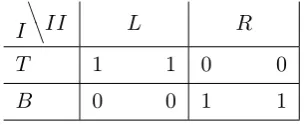
An easy example of a game with multiple equilibria is the Coordination Game3, illustrated by Figure 1.2. Each player receives 1 when the players

I

\

\II L R

T 1 1 0 0

B 0 0 1 1

Figure 1.2: Coordination Game.

choose the same strategies and 0 otherwise. The game has two Nash equi-libria in pure strategies, and a third in mixed strategies, when each player randomizes between his two pure strategies, assigning equal probability to each. The problems derive from the fact that there are two optimal choices for the players and the strategies are choosen simultaneously, so the players cannot effectively coordinate themselves.

Battle of the Sexes

One well-known example of a game with multiple equilibria is the Battle of the Sexes, illustrated by Figure 1.3. Two players wish to go to an event together, but disagree about whether to go to a football game or to the

3

(21)

I

\

\II F B

F 2 1 0 0

B 0 0 1 2

Figure 1.3: Battle of the Sexes.

ballet. Each player gets a utility of 2 if both go to his (or to her) preferred event, a utility of 1 if both go the other’s preferred event, and a utility of 0 if the two are unable to agree and stay at home or go out individually. The game has three equilibria: two in pure strategies, (F, F) and (B, B), and one in mixed: player I plays F with probability 2₃ (andB with probability

1

3), and player II plays F with probability 1

3 (andB with probability 2 3).

If two players have not played the battle of sexes before, there is no obvious way for the players to coordinate their expectations. However, the theory of focal points of Schelling (1960) suggests that in some real-life situations, players may be able to coordinate on a particular equilibrium using information abstracted away by the strategic form.

Prisoner’s Dilemma

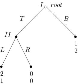
In the Prisoner’s Dilemma game, two suspects of a crime are put into se-parate cells. If both confess (strategy B and R, respectively) each will be sentenced to 2. If only one of them confesses, he will be freed and used as a witness against the other person, who will be sentenced to 3 years in prison. If both do not confess (strategy T and L, respectively), they will both be punished for a minor offense and spend 1 year in jail. Payoffs are represented by 3 minus the number of years spent in prison.

I

\

\II L R

T 2 2 0 3

B 3 0 1 1

Figure 1.4: Prisoner’s Dilemma.

(22)

strategy and theN E is not efficient. From here the interest reserved to Pri-soner’s Dilemma follows, since a reader might expect an efficient outcome, on account of rationality assumption of players. The Prisoner’s Dilemma repetion allows to draw up the paradox. As the game perpetuates, the play-ers are urged to cooperate (see Fudenberg and Tirole (1991) or Kreps et al. (1982).

Rock Paper Scissors

Rock Paper Scissors, depicted in the Figure 1.5 is a two player game. Each player has three strategies: rock, paper, and scissors. Rock breaks scissors, paper folds rock, and scissors cut paper. None of the pure strategy profiles constitute an equilibrium. The game has a unique symmetric equilibrium in mixed strategies: playerI playsR with probability 1₃,S with probability

1

3, andP with probability 1

3, and player II the same mixed strategy.

I\\II R P S

R 0 0 −1 1 1 −1

P 1 −1 0 0 −1 1

S −1 1 1 −1 0 0

Figure 1.5: Rock Paper Scissors.

RSP is a three player game with no pure strategy equilibria.

1.2

Games in Extensive Form

(23)

distributions over any exogenous events is represented by moves of Nature, eventually. In the following Sub-section we transfer, for completeness, the formal definition, some details of which are not essential for the rest of the work.

1.2.1 Extensive Game with Perfect Recall

We now formally define a finite game form in extensive form.

Definition 11. (Kuhn (1953)) A finite extensive game form is

Γ = (V, D, r, N,P,U,M, E, φ,(4k)k∈N), where:

1. (V, D, r) is a finite tree4 (V, D) with root r.

V denotes the tree node (or vertex) set, D the tree branch set, Z the terminal node set, and e X=V\Z the decisional node set.

2. N = {0,1, . . . , n} is the finite player set. 0 represents Nature. We assume that the random player can move only in r.

3. P = (Pk)k∈N∗ is a subdivision in disjoint subsets of X, also empty.

Pk are the set of pertinent nodes to playerk, that is the nodes in which k has to move.

4. U = (Uk,j)k∈N∗_,j_∈_Jk is, for each player k, a partition ofP_k in a family

of setsUk,j, Jk is a set of indices.

Uk,j are the nodes pertinent to player k, such that, when the player is one of them, who is not able to distinguish in which node he is.

5. A is, fork6= 0, a family of sets Ak,j, one for each of Uk,j.

In correspondence with a node of an information setUk,j, playerkhas to choose an action between those contained in Ak,j.

6. E is the set of possible final outcomes of the game.

7. φ:Z −→E associates to each terminal node an outcome.

8. (4k)k∈N represents a family of total preorder onE which represent the preferences for final outcomes of the game.

4

(24)

From here onwards, Γ denotes a game form, U(Γ) a partition ofX(Γ), i.e. each terminal node is also an information set, Ai(Γ) the actions available

to playeri,A(u) the action available to him in information setu, that is in A(u)⊆Ai,Ui(Γ) the information sets belonging to a player i∈N, (Γ, h) a

game in extensive form, andG(Γ) the set of games with game form Γ. Definition 12. An information set u is a class of pertinence nodes of a player such that

• all nodes inuhave the same number of outgoing branches, and there is a given one-to-one correspondence between the sets of outgoing branches of different nodes inu;

• every directed path in the tree from the root to a terminal node can cross each u at most once.

Grafically the dashed line connects the nodes belonging to the same infor-mation set.

Definition 13. A game is of perfect information if all the information sets are singletons.

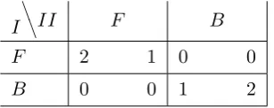
In a game of perfect information, there are no simultaneous moves, and at each decision point the player knows which choice has previously been made. The Figure 1.6 depicts a game with perfect information and a game without perfect information.

(25)

Unilateral Commitments 11 I c L M R H H H H H H H H H H x s II

A A A A A

y s II A A A A A

l1 r1 l2 r2

s 2 2 s 3 1 s 0 2 s 0 2 s 1 1 I c L M R H H H H H H H H H H x s A A A A A y s A A A A A

l r l r

II s 2 2 s 3 1 s 0 2 s 0 2 s 1 1

Figure 1.6: Games in extensive form with and without perfect information.

Almost all games in economics literature are games of perfect recall.

Definition 14. A game is of perfect recall if no player ever forgets any information he once knew, and all players know the actions they have chosen previously.

(26)

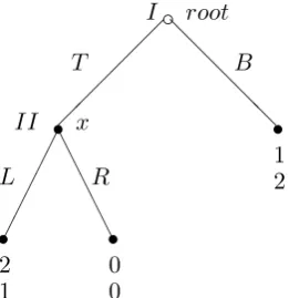
I c root @

@ @

T B

s

II A

A A

L R

s

2 1

s

0 0

s

1 2

Figure 1.7: Game in extensive form.

In the Figure 1.9, playerI makes his choice knowing the initial node, chosen by Nature (When a game involves Nature, the exogenous probabilities are displayed in brackets). If playerI choosesdand playerIIchoosesD, player I has to move again in the information set{x, y}, but he has forgotten the Natura choice, information he had at his disposal.

1.2.2 Behavior strategy profile

A pure strategy of a player is a complete plan for his choices in all possible contingencies in the game, that is at all his information sets. A mixed strategy means that the player chooses, before the beginning of the game, one such comprehensive plan at random, according to a certain probability distribution. An alternative method of randomization for the player is to make an independent random choice at each one of his information sets. That is, rather than selecting, for each information set, one definitive choice, as in a pure strategy, he specifies instead a probability distribution over the set of choices there. Moreover, the choices at different information sets are (stochastically) independent. These randomization procedures are called behavior strategies.

(27)

Unilateral Commitments 13 I c L R @ @ @ @ @ s A A A A A s A A A A A

l r l r

II s I s s s

s s s s s s

Figure 1.8: Game of non-perfect recall.

information set u, that is in A(u)⊆Ai bi :Ai −→[0,1] s.t.

X

a∈A(u)

bi(a) = 1, u∈Ui .

We denoteB(Γ) =

n

Q

i=1

Bi(Γ) the set of behavior strategy profiles of a gameG

or a game form Γ, and, with a slight abuse of notation,hi(b) the (expected)

payoff to player iwhen b∈B(Γ) is played.

Definition 16. A behavioral strategy profile b∈ B(Γ) is completely mixed if at each information set all the choices are taken with positive probability.

Thus the beliefs associated with a completely mixed strategy profile are completely determined by Bayes rule (see Section 1.4.3).

1.3

Games in Coalitional Form

(28)

c

N

[1₃] [2₃]

s

I

d

s I

d

s s

D D

II

s

I

s

s s

s s s s

Figure 1.9: Game of non-perfect recall.

Definition 17. A cooperative n-person game in coalitional form is an or-dered pair

hN, vi

where N = {1, . . . , n} is the set of players, and v : 2N −→ _R is a map, which assigns to each coalition S ∈ 2N a real number, such that v(∅) = 0.

v is called the characteristic function of the game and v(S) the value or the worth of coalitionS.

A game in coalitional form (or characteristic function) may represent very different situations, for example it can model a simple voting game where v associates to a winning coalition the value 1 and to a losing coalition the value 0, or an economic market that generates a cooperative game.

Example 1. (Glove game) LetN ={1, . . . , n}be divided into two disjunct subsetsL and R. Members of L possess a left hand glove, members ofR a right hand glove. A single glove is worth nothing, a right-left pair of gloves 1. This situation can be modeled by an n-person game hN, vi, where, for eachS ∈2N,

v(S)= min. {|L∩S|,|R∩S|}.

(29)

• Transferable utility games (TU) (also called Games with Side Pay-ments). The members of a coalition S can arbitrarily divide among themselves the amountv(S) which S can get. So a TU-game is of the form

v(S) ={(xi)i∈Ssuch that

X

i∈S

xi 6v(S)}.

• Non-transferable utility games (NTU), the games without transferable utility.

But these questions are not within our terms of references.

For completeness, we recall the Pure Bargaining games (PB). In these games only the grand coalition matters. Here, for allS 6=N,

v(S) ={(xi)i∈Ssuch that xi 60,∀i∈S}.

But these questions are not within our terms of references.

1.3.1 TUIC games

The TUIC games represent a simple model which allows embedding a coo-perative game of cost allocation in a richer structure, so that it is possible to take in account that cost information is expensive to get. In this structure, we can discuss how to balance on one hand the costs imposed by information requirements, on the other the loss of fairness when one tries to reduce these costs to the minimum. A T U IC-game is a family ofT U-game, indexed by a parameter t ∈ T, with information costs χt, and ordered by a transitive

and irreflexive relation ≺on T. In addition to the function ct of T U-game Gt, there is an extra costχtbringing the necessary information on the cost

to getct. For exampleχtis the additional cost to pass from a modelt1 ∈T

to anothert2 ∈T or to choose the functionct. Moreovert1 ≺t2 means the

model t2 has more information w.r.t. model t1 and ct2 approaches better the cost function thanct1.

Definition 18. A TUIC game is

hN, T,(ct)t∈T,(χt)t∈T,≺i,

where N is a finite set of players,T is a set of parameters (models), whose elements provide the needed information to have a TU game, ct:P(N)−→

(30)

1.4

Special classes of equilibria

1.4.1 Non-belief-based equilibria

The classic equilibrium concepts not based on beliefs are the Nash equi-librium and some of its refinements, such as the subgame perfect equili-brium (Selten (1965)), the perfect equiliequili-brium (Selten (1975)), the proper equilibrium (Myerson (1978)), the persistent equilibrium (Kalai and Samet (1984)), the essential equilibrium (Wu Wen-Ts¨un and Jiahg Jia-He (1962)), and the regular equilibrium (Harsanyi (1973)). We have also defined the NE in Subsection 1.1.3. Here, we introduce only the subgame perfect equi-librium in Subsubsection 1.4.1 and the perfect equiequi-librium in Subsubsection 1.4.1, since the others wander off the matter of this thesis.

Selten (1965), in order to discard those NE, possible if some players give credit to irrational (that is, non-maximizing) plan of the others, intro-duced the subgame perfect equilibrium, that is a NE which induces a NE in each subgame. But a subgame perfect equilibrium may also be non sen-sible, in the sense that it prescribes a choice non-maximizing the expected payoff. Selten (1975), to eliminate unreasonable subgame perfect equilib-ria, assumes that there is always a small probability that a player will take a choice by mistake, with the consequence that every choice will be taken with a positive probability. Therefore, in an extensive game with mistakes (a so called perturbed game), every information set will be reached with a positive probability. Then, an equilibrium of this game will prescribe ratio-nal behavior at every information set. Assuming that mistakes occur only with a very small probability leads to define a perfect equilibrium, that is an equilibrium obtained as a limit point of a sequence of disturbed games in which the mistake probabilities go to zero. Hence, an equilibrium is perfect if the equilibrium strategy of each player is not only optimal against the equilibrium strategies of his opponent, but if it is also optimal against some slight perturbations of these strategies.

Subgame Perfect Equilibria

(31)

We consider the game due to Selten (1975) in Figure 1.10. It is an

I c root @

@ @

T B

s

II x

A A

A

L R

s

2 1

s

0 0

s

1 2

Figure 1.10: Selten game.

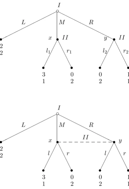
extensive game with perfect information. In order to identify the Nash equilibria, it is more convenient to analize the Selten game in strategic form, see Figure 1.11. The game has two NE (T, L) and (B, R), with payoff (2,1)

I

\

\II L R

T (2,1) (0,0)

B (1,2) (1,2)

Figure 1.11: Selten game in strategic form.

(32)

player a sub-optimal choice? The equilibrium (B, R) does not predict that II plays R, since the choiceB concludes the game andII has not to move. In general, a Nash equilbrium can predict non optimal choices on part of players in nodes of the tree not reached, if the equibrium profile is played. Again, the threat is not credible since ifI disregards the threat and playsT, thenII will play L, following his rationality. So, using the extensive form, we have shown that not all the Nash equilibria are the same. This leads to the definition of subgame perfect equilibrium orSP E by Selten (1965).

The argument used to exclude the equilibrium (B, R) in the Selten game in Figure 1.10 generalizes to all games with perfect information. Since in a non-cooperative game there are no possibilities for commitment, once the decision point x is reached, the part of the game tree which does not come afterx has become strategically irrelevant and, therefore, the decision atx should be based only on the part of the tree which comes afterx. This implies that for games with perfect information only those equilibria which can be found by inductively working backwards in the game tree, are sensible, i.e. self-enforcing. Using the backward induction principle, we get all the SPE of an extensive game.

Sequential rationality and subgame-perfectness are backward induction principles for the analysis of games in extensive form, because they require that any predictions that can be made about the behavior of players at the end of a game are supposed to be anticipated by the players earlier in the game.

Perfect Equilibria

(33)

Definition 19. Let G= (Γ, h) be an extensive game. Let εbe a function

ε:Ai −→(0,1]

which assigns to every choice a in G a positive number ε(a) such that, for every information set u∈Ui,

X

a∈A(u)

ε(a)<1.

The perturbed gameGε ∈ G(Γ)is the extensive gameGin which every player

i∈N is only allowed to use behavior strategies bi which satisfy

(bi)u>ε(a),

for allu∈Ui and a∈A(u).

LetGεbe a perturbed game and letBεbe the set of admissible strategy profiles inGε. An equilibrium ofGεis an admissible strategy profileb∈Bε which prescribes a best reply at every information set, i.e.

hi(bu) = max b0_i∈Bε i

hi(b−i, b

0

i)u,

for each i∈N and each u∈Ui. An equilibrium ofGε is perfect if it is still

sensible to play this equilibrium if slight mistakes are taken into account.

Definition 20. Let G be a game in extensive form. A behavioral strategy profileb is a perfect equilibrium of G if

b −→b, as →0,

that is, b is a limit point of a sequence of equilibria of perturbed gameGε.

In the game of Figure 1.12, only the equilibrium (R, r) is perfect. In a perturbed game associated with this game, playerI will take the choicesM and R with a positive probability (if only by mistake) and, therefore, the information set of playerII will actually be reached, which forces playerII to playr.

Theorem 1. (Selten (1975)) Every finite game possesses at least one perfect equilibrium.

(34)

I c L M R H H H H H H H H H H x s A A A A A y s A A A A A

l r l r

II s 2 2 s 1 1 s 0 2 s 0 0 s 3 1

Figure 1.12: G.

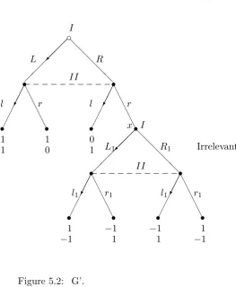
To illustrate the difference between the two concepts, let us consider the gameG0, in Figure 1.13, obtained with a slight modification of game G in Figure 1.12. As before, player II has to play r. For player I, both R andL are the best replies againstr. Therefore, in a sequential equilibrium, playerI can play any combination ofRandL. The only perfect equilibrium, however, is (L, r), since if player I plays L, he is sure of getting 3, whereas if he plays R, he can expect only slightly less than 3 since player 2 with a small probability will make a mistake and playl.

1.4.2 Belief-based equilibria

In this subsection, we extend the notion of subgame perfect equilibrium to extensive game with imperfect information. We focus on the concept of Sequential Rationality, and some of its refinements, such as Sequential Equilibrium and Weak Perfect Bayesian Equilibrim.

We recall that a Subgame Perfect Equilibrium of an extensive game with perfect information is a strategy profile for which the strategy of each player, given the strategies of the others, is optimal at any contingency in which it is his turn to take an action, also in tree nodes not reached by game. The natural extension of this idea to extensive games with imperfect information leads to the following requirement.

(35)

Unilateral Commitments 21 I c L M R H H H H H H H H H H x s A A A A A y s A A A A A

l r l r

II s 3 2 s 1 1 s 0 2 s 0 0 s 3 1

Figure 1.13: G0.

In the extensive game Gwith imperfect information in Figure 1.14, the requirement that each player’s strategy be optimal at every information set eliminates a NE.

I c L M R H H H H H H H H H H s A A A A A A A A U s A A A A A A A A U

l r l r

II s 2 2 s 3 1 s 0 0 s 0 2 s 1 1

Figure 1.14: G.

(36)

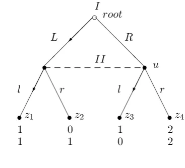
two NE: (L, r) and (M, l), both of which are subgame perfect. If player I adheres to equilibrium (L, r), then the information set of player II is not reached. However, if it is reached (playerI choosesM orL), the strategyr is dominated by strategyl. For any specification of playerII’s beliefs about the probability ofM andR when playerI deviates and does not playL, the optimal strategy of player II is to play r. Then (L, r) does not satisfy the condition of the extension, while the equilibrium (M, l) does. The extensive game with imperfect information G0 in Figure 1.16 has a NE (L, r) that is not ruled out by an implementation (?), since optimal strategy of player II in the event that his information set is reached depends on his beliefs about the history that has occurred. The strategyr is optimal ifII assigns probability of at most 1₂ to the history M, while l is optimal if he assigns probability at most 1₂ to this history. His belief cannot be derived from the equilibrium strategy, since (L, r) assigns probability zero to his information set being reached.

The solution for the extensive games studied in this section consists of two components: a strategy profile and a belief system.

Definition 21. A system of beliefs µ over X(Γ)\Z(Γ) is a function

µ:X(Γ)\Z(Γ)−→[0,1]

such that, for eachu∈U(Γ),

X

x∈u

µ(x) = 1.

That is, a belief system consists of a collection of probability measures, one for each information set of the game.

Definition 22. An assessment in an extensive game is a pair

(b, µ),

where b= (bi)i∈N is a behavioral strategy profile, and µa system of beliefs .

1.4.3 Bayes Rule

(37)

Definition 23. A probability measure on Ω is a function

P : 2Ω−→[0,1],

such that

i)P(∅) = 0, , ii)P(Ω) = 1, and

iii)f or each E, F ∈Ωs.t. E∩F =∅, P(E∪F) =P(E) +P(F). Definition 24. The conditioned probability of the event E given the event

F is

P(E|F)=. P(E∩F) P(F) .

In plain words, we restrict the sample space toF and then we calculate the probability of eventE.

Since P(F)∈[0,1],

P(E|F)> P(E∩F). Theorem 3. Let E, F be two events. Then,

P(E∪F) +P(E∩F) =P(E) +P(F).

Theorem 4. LetF1, . . . , Fm be mutually disjoint and complementary events, that is,Fi∩Fj =∅for eachi, j= 1, . . . , mwithi6=j, andF1∪. . .∪Fm = Ω. Then, for each event E,

P(E) =P(E|F1)P(F1) +. . . P(E|Fm)P(Fm).

Theorem 5 (Bayes theorem). Let E, F be events, then

P(E|F)P(F) =P(F|E)P(E).

Corollary 1 (Bayes rule). Let F1, . . . , Fn be mutually exclusive and ex-austive events and let E be an arbitrary events of sample space such that

P(E)6= 0, then

P(F1|E) =

P(F1)P(E|F1)

P(F1)P(E|F1) +. . .+P(Fm)P(E|Fm) .

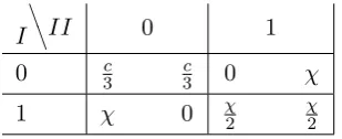
We consider the game in Figure 1.15 and we assume player I choosesT with probability 1₃ and B with 2₃, and playerII chooses t with probability

1

4, andd with 3

4. During the game, the node x of information set of player

III is reached with probability a priori 2₃, while the nodeywith probability a priori 1₄. A priori 1−P(T t) = 1− 1

3 1

4 = 1− 1 12 =

11

12 is the probability

(38)

c

I

B T

t II_s

b

x s A A

A A

A

y

s

A A

A

l r l r

III

s

3 3 0

s

4 4 4

s

1 1 1

s

5 5 0

s

2 2 2

Figure 1.15: Bayes rule application.

Sequential Rationality

Definition 25. An assessment (b, µ) is consistent if

(b, µ) = lim

n−→∞(b

n_{, µ}n₎_,

that is, it is the limit of a sequence of assessments(bn, µn)n∈_Nsuch that each

bn is completely mixed, each µn results from bn using Bayes rule.

The idea for consistent condition is that the probability of the events, con-ditioned on events with probability zero, approximates probabilities raised by strategies which assign positive probability to each actions.

Definition 26. An assessment (b, µ) is sequentially rational if, for each player i ∈ N and each information set u ∈ Ui(Γ) the strategy bi of the player i who has to move is the best replay, assegned his beliefs and the strategies of his opponents.

Sequential Equilibrium

Definition 27. An assessment (b, µ) is a sequential equilibrium of a finite game in extensive form with perfect recall if it is sequentially rational and consistent.

(39)

Unilateral Commitments 25 I c L M R H H H H H H H H H H x s A A A A A A A A U y s A A A A A A A A U

l r l r

II s 2 2 s 3 1 s 0 2 s 0 2 s 1 1

Figure 1.16: G’.

The assessment (b, µ) where

b= (b1, b2), b1 =L , b2=r , µ(x) =α , µ(y) = 1−α , ∀α∈(0,1)

is consistent since

(b, µ) = lim

n−→∞(b

n_{, µ}n₎_,

where

bn₁ = (1− 1

n, α 1

n,(1−α) 1 n), b

n

2 = (

1 n,1−

1

n), µ(x) =α , µ(y) = 1−α ,∀n. Ifα≥ 1₂, then (b, µ) is sequentially rational, since 2α+1(1−α)≥α+2(1−α). So (b, µ) is a sequential equilibrium.

Proposition 1. Each finite extensive game, with perfect recall, has a se-quential equilibrium.

Proposition 2. If (b, µ) is a sequential equilibrium, then b is a Nash equi-librium.

Proposition 3. In an extensive game with perfect recall, (b, µ) is a sequen-tial equilibrium if and only if bis a subgame perfect equilibrium.

Weak Perfect Bayesian Equilibrium

Definition 28. Let G= (Γ, h) be an extensive game. An assessment(b, µ)

(40)

(41)

Unilateral Commitments 27 I c L M R H H H H H H H H H H x s A A A A A A A A U y s A A A A A A A A U

l r l r

II s 2 2 s 3 1 s 0 2 s 0 2 s 1 1

G and(b, µ)

I

c

1− 1

n α 1

n (1−α)

1 n H H H H H H H H H H α s A A A A A A A A U

1−α

s A A A A A A A A U 1

n 1−

1

n

1

n 1−

1 n II s 2 2 s 3 1 s 0 2 s 0 2 s 1 1

G and(bn, µn)

(42)

(43)

Chapter 2

Potential game

2.1

Introduction

Monderer and Shapley (1996) introduced, for games in strategic form, three nested classes of potential games: the ordinal potential games, the weighted potential games, and the exact potential games (or in short potential games). The basic point of these classes is the existence of a real-valued function P, called potential function, on the strategy space, which measures alone the incentive of each player to deviate from a strategy. In the case of ordinal potential games, P gives only indications whether the deviation increases or decreases the payoff, while P for a weighted potential games values the weighted gap of the deviation, andP for an exact potential game measures the exact gap of the deviation. In this work, we will mainly deal with last class, that is with exact potential games (or in short potential games).

The potential function is not only an useful tool to analyze equilibrium properties of potential games, since the incentives of all players are mapped into only one function, but also P provides the necessary information for the determination of the Nash equilibria: a strategy profile is a NE if every unilateral deviation from it decreases the value of the potential function. We consider, for example, the Prisoner DilemmaGand the functionP depicted in Figure 2.1. The payoff change of a player, which unilaterally deviates, exactly matches the change in functionP. For example, if playerIIdeviates from (T, L) to (T, R), his payoff increases by 3−2 = 1 as well asP increases by 1−0 = 1. For this reasonP is called an exact potential of the gameG. We underline thatP is not the unique potential ofG. Another potential for G is P0, illustrated in Figure 2.2. In fact, the exact potential games enjoy

(44)

I

\

\II L R

T 2 2 0 3

B 3 0 1 1

L R

T 0 1

B 1 2

G P

Figure 2.1: Game and Potential.

L R

T 2 3

B 3 4

P0

Figure 2.2: P’.

the property that two potentials are different in a constant. Again, (B, R) is the NE since every unilateral deviation from this strategy profile decreases the value of the potential function. Thus, the information concerning pure NE accrues to a potential function.

Moreover, if strategy spaces are finite, the potential game has at least an equilibrium in pure strategies. A point of maximum forP, which exists since the product of finite space strategies is finite, is also a point of equilibrium forG.

There are various analogies with the physical concept of potential not only in the term and in the possibility of replacing n payoff functions (a vector field) with one potential function (a scalar field), but also in the fact that, if strategy spaces are finite, the “discret” circulation is always zero. If the strategy spaces are, instead, intervals of real numbers and each pay-off function is twice continuously differentiable, then the Schwarz theorem applies to potentialP and moreover, P is expressed by the integral of the partial derivatives of each payoff (see Monderer and Shapley (1996)).

(45)

their payoff depends on the number of players choosing the same alternative. Moreover, Monderer and Shapley (1996) showed that the class of congestion games coincides, up to an isomorphism, with the class of finite potential games.

This Chapter is organized as follows. In Section 2.2, we introduce po-tential functions, popo-tential games, and the relative properties. In Section 2.4 we study the characterization of exact potential games by splitting them into coordination games and dummy games. In Section 2.3, we intorduce congestion game in order to have the formula of potential function. Finally, in Section 2.5, we investigate symmetric games and we present our results. The first result establishes a symmetric game with only two strategies is a potential game and then it has a pure Nash Equilibrium. The originality lies in being a potential game, since Cheng and other (2004) has already showed that a symmetric game with only two strategies has a pure Nash equilibrium. The second one provides how all the NE of a symmetric, binary game are deduced from its potential function.

2.2

Potential game and potential function

This section defines ordinal potential game, exact potential games, surveys some simple results, and provides two characterizations of exact potential games.

Let G=hX1, . . . , Xn, u1, . . . , unibe a n-person strategy game.

Definition 30. [Monderer and Shapley (1996)] An ordinal potential for G

is a function P :

n

Q

i=1

Xi → R such that, for all i ∈ N, x−i ∈ X−i, and xi, yi∈Xi,

sgn(ui(xi, x−i)−ui(yi, x−i)) =sgn(P(xi, x−i)−P(yi, x−i)). sgn(x) denotes the sign ofx, namely +1,−1 or 0.

Definition 31. An exact potential (or, briefly, a potential) for Gis a

func-tion P :

n

Q

i=1

Xi → R such that, for all i ∈ {1, . . . , n}, x−i ∈ X−i, and xi, yi∈Xi,

ui(xi, x−i)−ui(yi, x−i) =P(xi, x−i)−P(yi, x−i).

(46)

Definition 32. A game admitting an ordinal or an exact potential function is called an ordinal or an exact potential game respectively (or, briefly, a potential game).

It is clear that the class of exact potential games is a proper subset of the class of ordinal potential games.

Again, a function may be a potential function or an ordinal potential one. For example,P is a potential for the Prisoner’s DilemmaGand at the same time it is an ordinal potential for the gameG0 described in Figure 2.3.

I

\

\II L R

T 2 3

B 3 4

P

I

\

\II L R

T 2 2 0 3

B 3 0 1 1

I

\

\II L R

T 2 2 0 3

B 3 0 1 1

G G0

Figure 2.3: P is a potential for Gand an ordinal potential forG0.

The next lemma characterizes the equilibrium set of an ordinal potential game.

Lemma 1. Let P be an ordinal potential for G=hX1, . . . , Xn, u1, . . . , uni. Then the equilibrium set ofG coincides with the equilibrium set of the game

hX1, . . . , Xn, P, . . . , Pi. That is,

(x1, . . . , xn) is a NE for G⇔ P(xi,x−i)>P(y,x−i)∀i∈N,∀y∈Xi.

Consequently, if P admits a maximal value in n

Q

i=1

Xi, then G has a pure

strategy equilibrium.

Corollary 2. Every finite ordinal potential game G has at least one pure Nash equilibrium.

(47)

Lemma 2. Let P1 and P2 be potentials for the game G. Then there is a

real constantc such that

P1(x1, . . . , xn)−P2(x1, . . . , xn) =c ∀(x1, . . . , xn)∈ n

Y

i=1

Xi.

The following theorem 6 characterizes potential game via a physical ap-proach, cyclicity on a simple closed path of length 4.

Definition 33. A path in n

Q

i=1

Xi is a sequence of strategy profiles

(xk₁, . . . , xk_n)k∈N,

such that, for everyk= 1,2, . . ., the strategies(xk₁, . . . , xk_n)kand(xk1−1, . . . , xk

−1

n )k, differ in exactly one, say the ith, coordinate, i.e., there is a unique player

i∈N such that

(xk_i, xk₋_i) = (y, xk₋−_i1) for some y ∈Xi\ {xki}.

(x0₁, . . . , x0_n) is called the initial point of path, and, if the sequence is finite, its last element(xl₁, . . . , xl_n) is called the terminal point of path, and the path is called finite.

Definition 34. A finite path is closed if (x0₁, . . . , x0_n) = (xl₁, . . . , xl_n).

Definition 35. A closed path is simple if, in addition, (xj₁, . . . , xjn) 6=

(xk₁, . . . , xk_n), for every 0 ≤ j 6= k ≤ l−1, that is, the strategy profiles are all distinct.

Definition 36. The length of a simple closed path is the number of distinct vertices in it.

That is, the length of the simple closed path (xk₁, . . . , xk_n)l_k₌₁ isl.

Definition 37. LetG=hX1, . . . , Xn, u1, . . . , unibe a game andπ= (xk1, . . . , xkn)k∈N

be a finite path. We set

I(π, u1, . . . , un)=.

X

k∈N

uik(xk1, . . . , xkn)−uik(xk1−1, . . . , xk

−1

n ),

where ik is the unique deviator at step k, that isxkik 6=x k−1

ik .

(48)

i) Gis a potential game.

ii) I(π, u1, . . . , un) = 0, for every finite closed pathπ.

iii) I(π, u1, . . . , un) = 0, for every finite simple closed pathπ.

iv) I(π, u1, . . . , un) = 0, for every finite simple closed pathπof length 4.

Corollary 3. G=hX1, . . . , Xn, u1, . . . , uni is a potential game if and only if

ui(xi, xj, x−{i,j})−ui(yi, xj, x−{i,j}) +uj(yi, xj, x−{i,j})+

−uj(yi, yj, x−{i,j}) +ui(yi, yj, x−{i,j})−ui(xi, yj, x−{i,j})+

+uj(xi, yj, x−{i,j})−uj(xi, xj, x−{i,j}) = 0,

where i, j are the active players, x−{i,j} ∈X−{i,j} is a fixed strategy profile

of the other players,xi, yj ∈Xi and xj, yj ∈Xj.

A typical simple closed path of length 4 is described in Figure 2.4.

u

A uD

u

B u C

-?

6

Figure 2.4: Simple closed path of length 4.

2.3

Congestion games

In this section we present the congestion mode, since we may extract the expression of potential from the construction (Rosenthal (1973)) of an exact potential function for a congestion game.

(49)

the same facility. The payoff to a player is the sum of the costs or ben-efits associated with each facility in his strategy choice, given the choice of the other players. By constructing a potential function for such conges-tion game, Rosenthal proved the existence of pure-strategy Nash equilibria. Moreover, Monderer and Shapley (1996) showed every finite potential games is isomorphic to a congestion game.

Before formalizing the definitions, we introduce a very simple example where two playersI and II are involved.

u

A u B

u

D u C

-c1(1)c1(2)

-c4(1)c4(2)

? c3(1)

c3(2)

?c2(1)

c2(2)

Player I has to go from point A to point C and player II has to go from point B to point D. Player I can travel viaB or via D and playerII via A or via C. The cost of using a segment depends on the number of users. We call 1 the segmentAB, 2 the segment BC, 3 the segmentAD and 4 the segmentDC,cj(1) denotes the cost of segmentj for a single user, andcj(2)

the cost ofj for each users if both use segmentj, wherej∈ {1, . . . ,4}. The associated congestion game is given by

I

\

\II L R

T (c1(2) +c2(1)) (c1(2) +c3(1)) (c2(2) +c1(1)) (c2(2) +c4(1))

B (c3(2) +c4(1)) (c3(2) +c1(1)) (c4(2) +c3(1)) (c4(2) +c2(1))

It is straightforward to see that this symmetric game is a potential game and so it has a Nash equilibrium in pure strategies. A potential is given by:

I

\

\II L R

T c1(1) +c1(2) +c2(1) +c3(1) c2(1) +c2(2) +c1(1) +c4(1)

(50)

Definition 38. A congestion model is described as a 4-tuple

hN, F,(Xi)i∈N,(cf)f∈Fi

where N = {1,2, . . . , n} is the set of players, F is the set of facilities

{1,2, . . . , f} involved, Xi ∈ P(F) is the set of pure strategies of player i, Xi 6= ∅, cf :N → R is the cost function of facility f so defined: for each k ∈ N, cf(k) denotes the costs to each user of facility f with precisely k users.

Definition 39. The congestion game corresponding to the congestion model is the cost game in strategic form hX1, . . . , Xn, C1, . . . , Cni where the cost for player iis

Ci(x1, . . . , xn) =

X

f∈xi

cf(|{r∈N s.t. f ∈xr}|).

The following theorem is the main result of Rosenthal (1973).

Theorem 7.(Rosenthal (1973)) Every congestion game is a potential game.

The potential functionP : Q

i∈N

Xi −→Ris defined by

P(x1, . . . , xn) =

X

i∈N

(X

f∈xi

cf(|{r ∈N s.t. f ∈xr}|).

Monderer and Shapley (1996) showed that the class of finite potential games coincides, up to an isomorphism, with the class of congestion games.

Definition 40. Let G1 =h(Xi)i∈N,(ui)i∈Ni andG2 =h(Yi)i∈N,(vi)i∈Ni be two game with the same set of playersN. G1 andG2 are isomophic if there

exist bijectionsφi :Xi −→ Yi, i∈ {1, . . . , n} such that for every i∈N and for every(x1, . . . , xn)∈

Q

i∈N Xi,

ui(x1, . . . , xn) =vi(φ1(x1), . . . , φN(xn)).

Proposition 4. (Monderer and Shapley (1996)) Every finite potential game is isomorphic to a congestion game.

2.4

Decomposition of exact potential games

(51)

I\\II L R

T 0 0 1 1

B 1 1 2 2

I\\II L R

T 2 2 −1 2

B 2 −1 −1 −1

Figure 2.5: PD is sum of coordination game and dummy game.

We can decompose the Prisoner’s Dilemma in Figure 1.4 into the sum of two games showed in Figure 2.5. It is immediate to see that, in the first game, the players have the same payoffs, while, in the second game, the payoffs of a player depend not on his choice, but on the strategy of his opponent. Formally, we present the following definitions.

Definition 41. A game G = hX1, . . . , Xn, u1, . . . , uni is a coordination game if there is a function u : Q

i∈N

Xi −→ R such that ui = u for each i∈N.

In a coordination game, players pursue the same goal, reflected by the iden-tical payoff functions. It is a game ofpure externality, in the sense that the strategy chosen by a player has effect only on the contestant.

Definition 42. A game G=hX1, . . . , Xn, u1, . . . , uni is a dummy game if, for eachi∈N and for eachx−i ∈X−i, there isk∈Rsuch thatui(xi, x−i) = k for each xi ∈X−i.

In a dummy game, each player has no reason to choose a strategy instead of another, since his payoff does not depend on his own strategy.

Facchini et al. (1997) provide this characterization of exact potential games by splitting them into coordination games and dummy games.

Theorem 8. Let G = hX1, . . . , Xn, u1, . . . , uni be a strategic game. G is a potential game if and only if, for each i= 1, . . . , n, there exist functions

ci : Q i∈N

Xi −→Rand di: Q i∈N

Xi−→R such that

i) ui =ci+di, for each i= 1, . . . , n,

(52)

Proof. The part ’if’ is obvious. The payoff function of the coordination game is an exact potential function of G. Let us consider the assertion ’only if’. LetP be an exact potential forG. For alli∈N, we haveui =P+ (ui−P).

Clearly, hX1, . . . , Xn, P, . . . , Pi is a coordination game. Let i ∈ N, x−i ∈ X−i, andxi, yi ∈Xi. Thenui(xi, x−i)−ui(yi, x−i) =P(xi, x−i)−P(yi, x−i)

implies ui(xi, x−i) −P(xi, x−i) = ui(yi, x−i) −P(yi, x−i). Consequently,

hX1, . . . , Xn, u1−P, . . . , un−Piis a dummy game.

2.5

Symmetric Game

Let G = hX1, . . . , Xn, u1, . . . , uni be a game in strategic form with player

setN ={1, . . . , n}. For convenience, in this section we use the notation (x, y, x−{i,j})∈Xi×Xj×X−{i,j},

where i, j ∈ N are the active players, x ∈ Xi is the strategy of player i, y ∈Xj is the strategy of player j, and x−{i,j} ∈X−{i,j} is a fixed strategy

profile of the other players.

Definition 43. G is a symmetric game if X1 =X2=. . .=Xn and

ui(x, y, x−{i,j}) =uj(y, x, x−{i,j}),

for x, y∈X1 and x−{i,j}∈X−{i,j}, ∀i, j∈N.

Definition 44. A symmetric strategy profile is a profile with all players playing the same strategy. If such a profile is a Nash equilibrium, it is a symmetric equilibrium.

Theorem 9. A symmetric binary game is a potential game.

Proof. For Corollary 3, the existence of an exact potential P is equivalent to the following condition:

ui(xi, xj, x−{i,j})−ui(yi, xj, x−{i,j}) +uj(yi, xj, x−{i,j})+

−uj(yi, yj, x−{i,j}) +ui(yi, yj, x−{i,j})−ui(xi, yj, x−{i,j})+

+uj(xi, yj, x−{i,j})−uj(xi, xj, x−{i,j}) = 0

Using symmetry,

(53)

we get:

ui(x, x, x−{i,j})−ui(y, x, x−{i,j}) +uj(y, x, x−{i,j})−uj(y, y, x−{i,j})+

+ui(y, y, x−{i,j})−ui(x, y, x−{i,j}) +uj(x, y, x−{i,j})−uj(x, x, x−{i,j}) =

=ui(x, x, x−{i,j})−ui(y, x, x−{i,j