Identification and Design of Closed loop Hydraulic system with 4/3 Servo valve.

(1)

Int. J. Adv. Res. Sci. Technol. Volume 4, Issue 7, 2015, pp.462-467.

International Journal of Advanced Research in

Science and Technology

journal homepage: www.ijarst.com

ISSN 2319 – 1783 (Print)

ISSN 2320 – 1126 (Online)

Identification and Design of Closed loop Hydraulic system with 4/3 Servo valve

Rajesh Kumar Mahapatra1*, Jagadish Chandra Pati1, GirijaSankar Rath2 and Priyabrata Biswal3

1

Department of Electrical Engineering, C.V.Raman College of Engineering, Bhubaneswar, India.

2_{Department of Applied Electronics & Instrumentation, C.V.Raman College of Engineering, Bhubaneswar, India.} 3

School of Minerals, Metallurgical and Materials Engineering, Indian Institute of Technology, Bhubaneswar, India. *Corresponding Author’s E-mail: rajeshavit@gmail.com

A R T I C L E I N F O A B S T R A C T

Article history:

Received Accepted Available online

09 Nov. 2015 22 Nov. 2015 26 Nov. 2015

Fluid power actuators play a vital role in the field of mechatronics. The controlling of electrohydraulic actuation system is important in the view of nonlinearity characteristics of hydraulic valves. In order to control the operation of valves, the controller should be designed as well as identification of the system is necessary to know the behavior of the system. This paper provides the derivation of transfer function for a electrohydraulic servo system by using transient response of the cylinder with respect to different set point with different loads .The performance of the system is analyzed using open loop without load, open loop with load, closed loop with load and it is observed that the performance of the system works better using closed loop. Also, in this paper the identification of the electrohydraulic servo system is done using transient response parameters and using Bode plot. It has been found that the poles & zeros of the system determined by the transient response & Bode’s Plot are nearly equal. For the transfer function derived from different conditions such as open loop, closed loop, with variable loads, the PID controller is also designed and the performance characteristics hold good with theoretical aspects.

Identification, Mechatronics, Electrohydraulic servo valve, Transient response,

Transfer function, Bode Plot , PID control

PAPER-QR CODE

Citation: Rajesh Kumar Mahapatra. et. al. Identification and Design of Closed loop Hydraulic system with 4/3 Servo valve,Int. J. Adv. Res. Sci. Technol. Volume 4, Issue 7, 2015, pp.462-467.

Introduction:

The range of applications of electrohydraulic servo system includes manufacturing systems, heavy duty material testing devices, hydraulic mini press machine, robotics, steel and aluminium mill equipment. In case of electrohydraulic actuation system, hydraulic power in conjunction with a servo valve is used to provide the desired forces and motion. The desired motion is achieved through a closed loop feedback control systemthat senses the actual deflection and corrects it until the desired position is achieved [1].

This paper reports identification of electrohydraulic servo system to which different sinusoidal inputs with constant amplitude 0.01volt at various frequencies ranges from 1Hz, 2Hz, 5Hz, 10Hz, 20 Hz, 100Hz, 500Hz, 1kHz are applied. The transfer function for the

electrohydraulic servo system was derived by using natural frequency ωnand damping ratio ζ with various

set points as well as providing different loads such as 1Kg, 5Kg, and 10Kg. Also, the frequency response in terms of Bode’s plot at different load conditions is observed. Then for given transfer function the PID controller has been introduced and performance characteristics in terms of rise time, settling time and peak time are discussed.

Electrohydraulic Servo System:

(2)

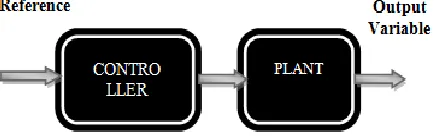
A servo or a servomechanism is a control system which measures its own output and forces the output to quickly and accurately follow a command signal and can be designed to control almost any physical quantities, e.g. motion, force, pressure, temperature, electrical voltage or current.

Fig.1:Block diagram for electrohydraulic servo system

Identification and Control of Electrohydraulic Servo System:

Hydraulic servo systems provide larger driving force as well as torque and higher speed of response with faster motion. Though it provides many advantages it exhibits nonlinearity [3]. In order to know the input-output relationship of components, it is required to derive the transfer function. The identification technique may involve time domain analysis in terms of transient response and frequency domain analysis. This paper uses both the time domain

approach & frequency domain approach for

identification of electrohydraulic servo system. Here, the electrohydraulic servo system consists the flow control valve, linear actuator, servo controller which can be an amplifier or gain and to the linear actuator various loads are given so that cylinder rod position in terms of transient response can be observed. By taking servo valve & linear actuator as a plant as well as a set point of 0.1 volt is given to the servo valve, the block diagram shown in fig.1 can be designed as an open loop block which is in fig.2. In open loop case, the loads are not connected to the linear actuator and the cylinder rod position has been observed. Then different loads like 1kg, 5 kg and 10 kg are given to the cylinder and therequired block diagram representation is shown in fig.3.

Fig. 2:Open loop Block diagram for electrohydraulic servo valve with linear actuator

Fig. 3:Open loop Block diagram for electrohydraulic servo valve with actuator connected to load

Fig. 4:Closed loop Block diagram for electrohydraulic servo valve with linear actuator

Fig. 5: Closed loop Block diagram for electrohydraulic servo valve with actuator connected to load

By connecting the output to the input with unity feedback, the open loop system shown in fig.2 and fig.3 can be designed into closed loop system shown in fig.4 and fig.5 respectively. From the closed loop response, the transient and steady state response has been analyzed by calculating maximum peak time, damping ratio and natural frequency with varying loads. The transient and steady state error analysis curve is shown in fig.6 which shows the characteristics such as rise time, settling time [4].

Fig. 6: Transient & steady state response analysis

The time response c(tp) can be as follows [4].

) 1 ( 1 ) sin 1 (cos

1 1 ) (

2 

  



 

r d r

d t

r e t t

t

c dr 

  



0 sin

1 cos

2 

 

 _dt_r _dt_r

  

) 2 ( 1

tan

2 

  

 d

r

dt 

   

Input Signal

Hydraulic Power Supply

Servo Contr oller

Flow Control

Valve

Linea r Actua

tor

L o a d

Displacemen t Transducer

Outpu t

(3)

Now, the rise time can be calculated using equation-3

) 3 ( tan

1 1 _

        

d d

r t

Peak Time

t

_p to reach the first peak of c(t)

) 4 ( 0 sin 0 1 ) (sin 0 ) ( 2 d p p d t n p d t t t t e t dt t

dc np

p                ) 5 ( 1 2

    n P T

Maximum overshoot Mp

) 6 ( 2 1 exp









     p m d p t t

Settling Time is given by

) 7 ( 1 tan sin 1 1 ) ( 2 1 2         _            t t t

c n _d

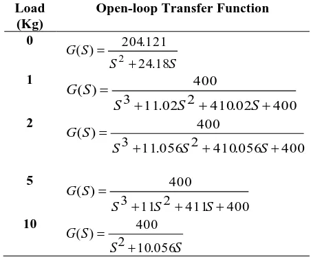
The open loop transfer functions have been derived using equation-1 to equation-7 and are given in table.1.

Table: 1.Open loop transfer function

Load (Kg)

Open-loop Transfer Function

0 S S S G 18 . 24 121 . 204 ) ( 2_  1 400 02 . 410 2 02 . 11 3 400 ) (     S S S S G 2 400 056 . 410 2 056 . 11 3 400 ) (     S S S S G 5 400 411 2 11 3 400 ) (     S S S S G 10 S S S G 056 . 10 2 400 ) (  

Then the identification technique involves analysis of frequency response of the system at different load conditions as well as to determine order of the system frequency characteristics of the system with feedback at different load condition were performed and the Bode’splot presented. In this paper the Bode diagram is

obtained by finding amplitude response-relationship between output and input amplitude with respect to excitation frequency. From the peak value, natural frequency ωn& damping ratio ζ were determined with

different load condition with the assumption that the system is a second order system.The resonant frequency ωr and the resonant peak Mr for carrying out bode plot

can be calculated using equation-8 [5].

) 8 ( 2 2 2 2 2 1 1 ) (                      n n j G     

Where ωn is natural frequency

ζ is the damping ratio.

With the derived transfer function for the electrohydraulic servo system, the 3-term controller or

integer PID controller implemented and the

performance of the system in terms of rise time, peak time and settling time has been discussed. The transfer function for PID controller in S-domain is given in equation-9 and the block diagram for the system is shown in fig.7.

Fig. 7: Block diagram for the PID controller

Simulation and Result:

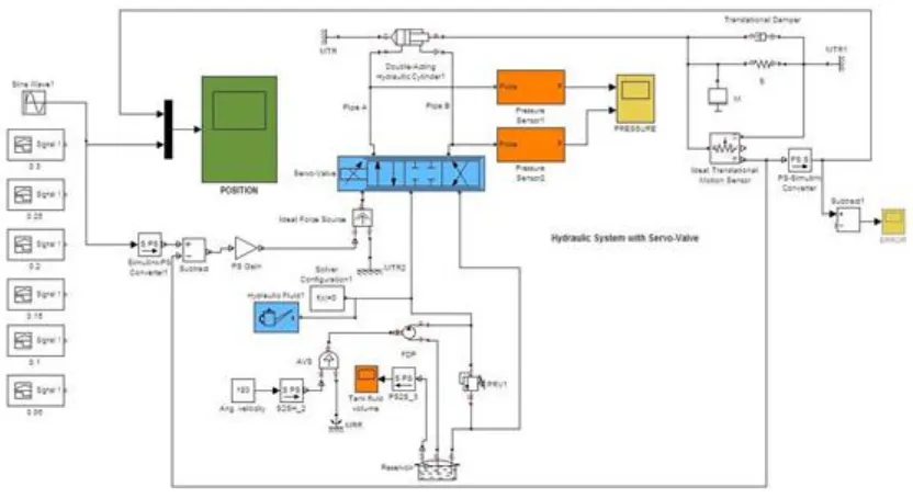
The electrohydraulic servo system shown in fig.1 has been designed and simulated using MATLAB-Simulink and is shown in fig.8 [7].It is simulated without feedback, with feedback & with load condition (mass is acting as load). It was observed when the input is more than 0.1 u(t) volts; the steady state response doesn’t go to 0.1m, it is due to limitation of actuating cylinder and is shown in fig.9. The stroke length is limited to 0.3 meter and the system is quick nonlinear.

(4)

Fig. 8:Electrohydraulic servo system in MATLAB-Simulink environment

Fig. 9:Cylinder position with no load in open loop

Fig. 10:Cylinder position with different load w.r.t 0.1u(t) in open loop condition

Table-3: Natural frequency & damping factor values

Load

( kg)

Maximu m point (dmax)

Peak time

(Tp)

Natural frequency

ωn

Damping

factor ζ

1 0.1232 0.3949 19.2562 0.2505

2 0.1232 0.3947 18.2581 0.2501

5 0.1232 0.3947 18.2595 0.2504

10 0.1232 0.3952 19.2601 0.2501

100 0.1233 0.3951 18.2600 0.2500

500 0.1238 0.3963 19.2409 0.2471

1000 0.1243 0.3985 17.2300 0.2393

The closed loop response of the electrohydraulic system with no load and with varied load is shown in fig.11 and from the response for different load condition poles & zeros of close-loop transfer function were obtained.

(5)

Then in order to obtain the frequency response of the system, a sinusoidal signal having varied frequency has been given to the electrohydraulic system at no load as well as different loads and correspondingly output peak amplitude has been calculated. The output response i.e. cylinder rod position at 20Hz frequency with feedback & no load is shown in fig.12.

Fig. 12: Cylinder rod position at Frequency 20Hz with feedback & without load

Table: 3.Gain at different frequency with no load

Frequency in Hz

Amplitude of output

Gain in dB

1 0.01 0

2 0.01 0

5 0.0101 0.086427476

10 0.0119 1.510939228

20 0.0199 5.977061528

50 3.9385×10-3 -8.093383004

100 9.5122×10-4 -20.43638966

200 2.6625×10-4 -31.49420767

500 5.0402×10-5 -45.91698966

1000 1.2783×10-5 -57.86734422

2000 4.3856×10-6 -67.15941964

In order to obtain Bode plot, the output value and the gain in dB w.r.t no load, 1k.g, 2kg, 5 Kg and 10 Kg are give in table no.3 table no.4, table no.5, table no.6 and table no.7 respectively.

Table: 4.Gain at different frequency with 1 kg load

Frequency in Hz

Output

amplitude Gain in dB

1 0.01 0

2 0.01 0

5 0.0102 0.172003435

10 0.0119 1.510939228

20 0.0199 5.977061528

50 3.9342×10-3 -8.102871319

100 9.3107×10-4 -20.62035333

200 2.8004×10-4 -31.05559862

500 5.1473×10-5 -45.76841038

1000 1.6615×10-5 -55.58999309

2000 2.7278×10-6 -71.2837495

Frequency in Hz

Output

1 0.01 0

2 0.01 0

5 0.0102 0.172003435

10 0.0119 1.510939228

20 0.02 6.020599913

50 3.9643×10-3 -8.036669751

100 9.2731×10-4 -20.65550114

200 2.7776×10-4 -31.12660593

500 6.5798×10-5 -43.63574614

1000 1.4393×10-5 -56.83697349

2000 5.4988×10-6 -65.19464152

Frequency in Hz

Output

1 0.01 0

2 0.01 0

5 0.0102 0.172003435

10 0.0119 1.510939228

20 0.0199 5.977061528

50 3.9516×10-3 -8.064540465

100 9.3033×10-4 -20.62725949

200 2.6865×10-4 -31.48605573

500 6.3171×10-5 -43.98978246

1000 2.0116×10-5 -53.92916746

2000 9.6097×10-6 -60.34824419

To determine order of the system frequency characteristics of the system with feedback at different load condition were performed and the Bode’s plot presented in fig.13 & fig.14.

Frequenc y in Hz

output

amplitude Gain in dB

1 0.01 0

2 0.01 0

5 0.0102 0.086427476

10 0.0127 1.510939228

20 0.0199 5.977061528

50 3.9453×10-3 -8.093383004

100 9.2892×10-4 -20.43638966

200 2.7365×10-4 -31.49420767

500 6.0259×10-5 -45.91698966

1000 1.1845×10-5 -57.86734422

(6)

Fig. 13: Bode plot with no load condition

Fig. 14.Bode plot for 5kg & 10 kg load

From the above Bode’s Plot all the corner frequency are determined. The ζ of complex corner frequency was determined by taking overshoot at the corner frequency.

Table-8: Poles and Corner frequency from Bodeplot

It has been found that the poles & zeros of the system determined by the transient response &Bode’s Plot are nearly equal (because of observational error). Therefore most expected Transfer Function is

) 9 ( 056 . 10 2

400 )

(

S S

S G

 

Then with derived transfer functions, the PID controllers for the system are designed and transient parameters are observed in the table no.9.

Table: 9.Transient parameters

Conclusion and Future Work:

This paper takes a case study of electrohydraulic servo valve which is connected to a cylinder and defined the performance of the servo system with varied loads not only in open loop case but also in closed loop case .Also, from the observation it has been found that the system performance is better in closed loop condition and PID controller designed. The identification of the system is done with both time domain and frequency domain approach.In future we can improve the performance of electrohydraulic system with nonlinearity conditions as well as design of fractional order controller to the system .Also, the system can be identified using fractional order synthesis.

References:

1. C.W.de Silva: Control Sensors and Actuators, Prentice Hall. New Jersey: 1989.

2. E. Papadopoulos, a systematic methodology for optimal component selection of Electro hydraulic servo systems International journal of fluid power, volume 5 ,number 3, November 2004 ,page 31-39.

3. Junpeng Shao, Zhangwen Wang,Jianying Lin and Guihua Han, “Model Identification and Control of Electro-Hydraulic position servo system”, International Conference on Intelligent Human-Machine systems and Cybernaics,pp.210-213,2009.

4. K. Ogata, Modern Control Engineering.3rd edition, PHI private Ltd, 2001

5. K.P.Ramchandran and M.S.Balasundaram, Mechatronics. Wiley India, New Delhi: 2008.

6. Matlab/Simulink, User’ s Manual, Mathworks 2007 7. Merritt, Herbert E., 1967, Hydraulic Control Systems,

Wiley, New York.

8. Walter, R. B., Hydraulic and Electro hydraulic Control system, Cliff, London, 1967

.

Load (in Kg)

Rise time (sec)

Settling time (sec)

Peak time (Sec)

No load 0.0308 0.101 1.09

1 0.684 2.22 1.09

5 0.685 2.22 1.08

10 0.074 0.242 1.06

Load(Kg) Poles Corner frequency(Hz)

Identification and Design of Closed loop Hydraulic system with 4/3 Servo valve.

International Journal of Advanced Research in

Science and Technology

Identification and Design of Closed loop Hydraulic system with 4/3 Servo valve

t









.

0

-45.9169

500

1

-44.3995

500

2

-45.7684

500

5

-43.6357

500