INTELIGENCIA ARTIFICIAL
http://journal.iberamia.org/
Probabilistic Extension to the Concurrent Constraint
Factor Oracle Model for Music Improvisation
Mauricio Toro
Universidad EafitCarrera 49 # 7 sur - 50, Medell´ın, Antioquia, Colombia [email protected]
Abstract
We can program a Real-Time (RT) music improvisation system in C++ without a formal semantic or we can model it with process calculi such as the Non-deterministic Timed Concurrent Constraint (ntcc) calculus. “A Concurrent Constraints Factor Oracle (FO) model for Music Improvisation” (Ccfomi) is an improvisation model specified on ntcc. Since Ccfomi improvises non-deterministically, there is no control on choices and therefore little control over the sequence variation during the improvisation. To avoid this, we extended Ccfomi using the Probabilistic Non-deterministic Timed Concurrent Constraint calculus. Our extension to Ccfomi does not change the time and space complexity of building the FO, thus making our extension compatible with RT. However, there was not a ntcc interpreter capable of RT to execute Ccfomi. We developed Ntccrt –a RT capable interpreter for ntcc– and we executed Ccfomi on Ntccrt. In the future, we plan to extend Ntccrt to execute our extension to Ccfomi.
Resumen
Podemos modelar un sistema de improvisaci´on musical de tiempo real (RT) en C++ sin una sem´antica formal o podemos modelarlo con un c´alculo de procesos como el c´alculo de procesos temporal, no determin´ıstico, con restricciones (ntcc). “Un modelo de improvisaci´on musical concurrente por restricciones basado en el Or´aculo de Factores (FO)” (Ccfomi) es un modelo de improvisaci´on especificado en ntcc. Como Ccfomi improvisa de una manera no determin´ıstica, no hay control sobre las escogencias que hace y por consiguiente, hay poco control sobre la variaci´on en las secuancias durante la improvisaci´on. Para evitar esto, proponemos extender Ccfomi usando el c´alculo de procesos temporal, no determin´ıstico, probabil´ıstico con restricciones. Nuestra extensi´on a Ccfomi no cambia la complejidad en tiempo y espacio del algoritmo de construcci´on del FO, haciendo nuestra extensi´on compatible con RT. Sin embargo, no hay un int´erprete para ntcc que sea cap´az de ejecutar Ccfomi en RT. Nosotros desarrollamos Ntccrt –nuestro int´erprete para ntcc capaz de RT– y ejecutamos Ccfomi en Ntccrt. En el futuro, planeamos extender Ntccrt para ejecutar nuestra extensi´on a Ccfomi.
Keywords: Factor oracle, concurrent constraints programming, ccp, machine learning, machine improvisation, Ccfomi, Gecode, ntcc, pntcc, real-time.
Palabras Clave: Or´aclulo de factores, programaci´on concurrente por restricciones, ccp, aprendizaje por com-putador, improvisaci´on musical por computador, Ccfomi, Gecode, ntcc, pntcc, tiempo real.
1
Introduction
There are two different approaches to develop multimedia interaction systems (e.g., machine improvisa-tion).
ISSN: 1988-3064(on-line) c
One may think that in order to implement real-time capable systems, those systems should be written directly in C++ for efficiency. In contrast, one may argue that multimedia interaction systems –inherently concurrent– should not be written directly in C or C++ because there is not a formalism to reason about concurrency in C++. We argue that those systems should be modeled using a process calculus with formal semantics and verification procedures, and execute those models on a real-time capable interpreter. That will be our definition for real-time in the rest of this document.
Garavel explains in [9] that models based on process calculi are not widespread because there are many calculi and many variants for each calculus, being difficult to choose the most appropriate. In addition, it is difficult to express an explicit notion of time and real-time requirements in process calculi. Finally, he argues that existing tools for process calculi are not user-friendly.
1.1
Motivation
Defending the calculi approach, Rueda et al. [27],[28] explain that using the semantics and logic un-derlying the Non-deterministic Timed Concurrent Constraint (ntcc) [17] calculus, it is possible to prove properties of thentccmodels before executing them and execute the models on antcc interpreter. We define soft real-time multimedia interaction means that the system reacts fast enough to interact with human players without letting them notice delays.
One may disagree with Rueda et al., arguing that although there are several interpreters for ntcc such as Lman [16] and Rueda’s Interpreter [28], there is not a generic interpreter to runntccmodels in real-time.
We agree with Rueda et al. about the way to develop those systems, but we also argue that currently there are nontccinterpreters capable of real-time. We argue, in agreement with Rueda et al.’s argument, that models based onntcc such as “A Concurrent Constraints Factor Oracle model for Music
Impro-visation” (Ccfomi) [28] are a good alternative to model multimedia interaction because synchronization
is presented declaratively by means of variable sharing among concurrent agents reasoning about infor-mation contained in a globalstore. However, due to non-deterministic choices, improvisation in Ccfomi can be repetitive (i.e., it produces loops without control). In addition, since Ccfomi does not change the intensity of the learned notes, Ccfomi may produce a sharp difference in the relative loudness between what a musician plays and what the improviser plays.
Process calculi has been applied to the modeling of interactive music systems. As an example, process calculi was proved succesful to model interactive scores [37] and Temporal Relations for Micro and Macro Controls [36]. Process calculi has also been used to model ecological systems, for instance, population models for dengue [38] and ecological systems [21].
Our main objective is extending Ccfomi to model probabilistic choice of musical sequences. We also want to show that a ntcc model can interact with a human player in soft real-time using a ntcc interpreter. For that reason, we developed Ntccrt, a generic real-time interpreter forntcc.
The rest of this introduction is organized as follows. First section, gives a definition of music improvi-sation. Second section, explains machine improviimprovi-sation. Third section, gives a brief introduction tontcc and presents systems modeled with ntcc. After explaining the intuitions about music improvisation, machine improvisation, and ntcc we explain our solution to extend Ccfomi in Section fourth section. Fifth section explains the contributions of this article. Finally, sixth section explains the organization of the following chapters.
1.2
Music improvisation
“Musical improvisation is the spontaneous creative process of making music while it is being performed. To use a linguistic analogy, improvisation is like speaking or having a conversation as opposed to reciting a written text. Among jazz musicians there is an adage, improvisation is composition speeded up, and vice versa,composition is improvisation slowed down.”[14]
1.3
Machine improvisation
Machine improvisation is the simulation of music improvisation by the computer. This process builds a representation of music, either by explicit coding of rules or applying machine learning methods. For real-time machine improvisation it is necessary to perform two phases concurrently: Stylistic learning
and Stylistic simulation. In addition, to perform both phases concurrently, the system must be able to
interact in real-time with human players [28].
Rueda et al. defineStylistic learningas the process of applying such methods to musical sequences in order to capture important musical features and organize these features into a model, and the Stylistic
simulation as the process producing musical sequences stylistically consistent with the learned style [28].
An example of a system running concurrently both phases isCcfomi, a system using the Factor Oracle (F O) to store the information of the learned sequences and thentcccalculus to synchronize both phases of the improvisation.
Thentcc calculus is a mathematic formalism used to represent reactive systems with synchronous, asynchronous and/or non-deterministic behavior. This formalism and its extensions have been used to model systems such as: musical improvisation systems [28] and an audio processing framework [29].
1.4
Our solution
To avoid a repetitive improvisation, we extendCcfomi with the Probabilistic Non-deterministic Timed Concurrent Constraint (pntcc) calculus [20] to decrease the probability of choosing a sequence previously improvised. This idea is based on the ProbabilisticCcfomi model [20] developed by P´erez and Rueda. That model, chooses the improvised sequences probabilistically, based on a probability distribution. Unfortunately, Probabilistic Ccfomi does not give information about how that probability distribution can be built nor how it can change through time according to the user and the computer interaction. Our model is the first pntcc model, as far as we know, where probability distributions change from a time-unit to another.
For instance, consider that our system can play in a certain moment the pitches (i.e., the frecuency of the notes)a,band cwith an equal probability. Then it outputs the sequence “aaba”. After that, it is going to choose another pitch. When choosing this pitch, chas a greater probability to be chosen than
b, andb has a greater probability to be chosen than abecause a was played three times andb once in the last sequence. Using this probabilistic extension, we avoid multiple cycles in the improvisation which can happen without control in Ccfomi.
On the other hand, to be coherent with the relative loudness on which the user is currently playing, we change the intensity of the improvised notes. This idea is based on interviews with musicians Riascos and Juan Manuel Collazos, where they argue that this is a technique they use when improvising and improves the “quality” of the improvisation, when two or more persons improvise at the same time.
For instance, if the computer plays five notes with intensities (measured from 0 to 127) 54, 65, 30, 58, 91 and the user plays, at the same time, four notes with intensities 10, 21, 32, 5; they are incoherence results because the user is playing low and the computer is playing loud. For that reason, our system multiplies its intensities by a factor of 0.29 (the relation of the average of both sequences) changing the intensities of the computer output to 16, 19, 9, 17, 26.
1.5
Contributions
• Ntccrt. A real-time capable interpreter forntcc[35]. Using Ntccrt, we executedCcfomi. Examples,
sources and binaries can be found at http://ntccrt.sourceforge.net. An article about Ntccrt is to be published this year.
• Gelisp. A new graphical constraint solving library for OpenMusic. We plan to use it in the future
1.6
Organization
The structure of this article is the following. In Chapter 1, we explain the background concepts. Chapter 2 focuses on the modeling ofCcfomito allow probabilistic choice of musical sequences. Chapter 3 explains the modifications toCcfomi to allow variation of the intensity of learned notes during the style simulation phase. Chapter 4 describes our model in pntcc. Chapter 5 explains the design and implementation of Ntccrt, our real-time interpreter for ntcc. Chapter 6 shows some results and tests made with the interpreter. Finally, in Chapter 7, we present a summary of this article, concluding remarks, and propose some future work.
2
Background
2.1
Concurrent Constraint Programming (CCP)
Concurrent Constraint Programming (CCP [31])is a model for concurrent systems. In CCP, a concurrent
system is modeled in terms of constraints over the system variables and in terms of agents interacting with partial information obtained from those variables. A constraint is a formula representing partial information about the values of some of the system variables. Programming languages based on the CCP model, provide apropagator for each user-defined constraint.
P ropagators can be seen as operators reducing the set of possible values for some variables. For instance, in a system with variablespitch1andpitch2taking Musical Instrument Digital Interface (MIDI)
values, the constraintpitch1> pitch2+ 2 specifies possible values forpitch1 andpitch2 (wherepitch1 is
at least one tone higher thanpitch2). In MIDI notation, each MIDI pitch unit represents a semi-tone.
The CCP model includes a set of constraints and a relation to know when a constraint can be deduced from others (named entailment relation|=). This relation gives a way of deducing a constraint from the information supplied by other constraints.
“The idea of the CCP model is to accumulate information in astore. The information on thestore
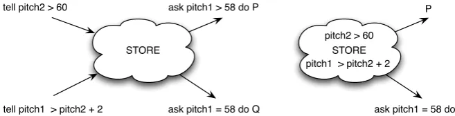
can increase but it cannot decrease. Concurrent processes interact with thestore by either adding more information or by asking if some constraint can be deduced from the current store. If the constraint cannot be deduced, this process blocks until there is enough information to deduce the constraint” [28]. Consider for instance four agents interacting concurrently (fig. 1). The processes tell (pitch1 >
pitch2+ 2) andtell(pitch2>60) add new information to thestore. The processesask(pitch1>58)do
P andask(pitch1= 58)doQlaunch processP andQ(P andQcan be any process) respectively, when
their condition can be entailed from the store. After the execution of the tell processes, process ask
(pitch1>58)doP launches processP, but the processask(pitch1= 58)doQwill be suspended until
its condition can be entailed from thestore.
STORE tell pitch2 > 60
tell pitch1 > pitch2 + 2
ask pitch1 > 58 do P
ask pitch1 = 58 do Q
STORE pitch2 > 60
pitch1 > pitch2 + 2 P
ask pitch1 = 58 do Q
Figure 1: Process interaction in CCP
Formally, the CCP model is based on the idea of a constraint system. “A constraint system is a structure< D,`, V ar >where D is a (countable) set of primitive constraints (or tokens),`∈D×Dis an inference relation (logical entailment) that relates tokens to tokens andV aris an infinite set of variables” [31]. A (non primitive) constraint can be composed out of primitive constraints.
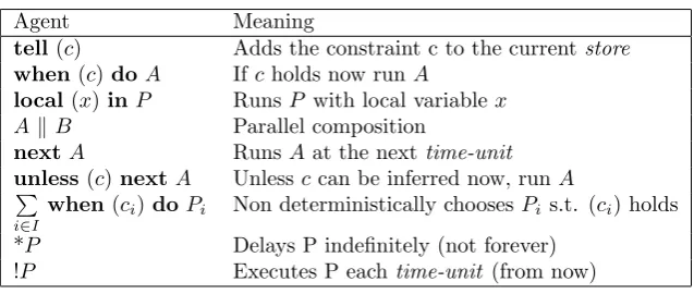
Agent Meaning
tell(c) Adds the constraint c to the currentstore when (c)doA Ifcholds now runA
local(x)inP RunsP with local variablex
Ak B Parallel composition
nextA RunsAat the nexttime-unit
unlessP (c)nextA Unlessccan be inferred now, runA
i∈I
when(ci)doPi Non deterministically choosesPi s.t. (ci) holds
*P Delays P indefinitely (not forever) !P Executes P eachtime-unit (from now)
Table 1: Ntcc Agents
domain (FD) constraint system provides primitive constraints (also called basic constraints) such as
x ∈ R, where R is a set of ranges of integers. On the other hand, finite set (FS) constraint system provides primitive constraints such as y ∈S, whereS is a set of FD variables and y is an FD variable. Constraints systems may also include expressions over trees, graphs, and sets.
Valencia and Rueda argue in [30] that the CCP model posses difficulties for modeling reactive sys-tems where information on a given variable changes depending on the interactions of a system with its environment. The problem arises because information can only be added to the store, not deleted nor changed.
2.2
Non-deterministic Timed Concurrent Constraint (
ntcc
)
Ntcc introduces the notion of discrete time as a sequence of time-units. Each time-unit starts with a store (possibly empty) supplied by the environment, thenntcc executes all processes scheduled for that
time-unit. In contrast to CCP, inntcc variables, changing values along time can be modeled. In ntcc
we can have a variablextaking different values alongtime-units. To model that in CCP, we would have to create a new variablexi each time we change the value of x.
Following, we give some examples of how the computational agents of ntcc can be used. The op-erational semantic of all ntcc agents can be found in Appendix ?? and a summary can be found in table 1. Using the tell agent with a FD constraint system, it is possible to add constraints such as
tell(pitch1 = 60) (meaning thepitch1 must be equal to 60) or tell(60 < pitch2 < 100) (meaning that
pitch2 is an integer between 60 and 100).
Thewhenagent can be used to describe how the system reacts to different events, for instancewhen pitch1= 48∧pitch2= 52∧pitch3= 55do tell(CM ayor=true) is a process reacting as soon as the pitch
sequence C, E, G (represented as 48, 52, 55 in MIDI notation) has been played, adding the constraint
CM ayor=trueto thestorein the currenttime-unit.
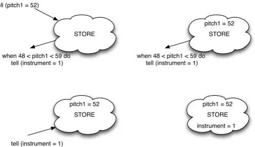
Parallel compositionallows us to represent concurrent processes, for instancetell(pitch1= 52)k
when 48 < pitch1 <59 do tell (Instrument = 1) is a process telling the store that pitch1 is 62 and
concurrently reacts whenpitch1 is in the octave -1, assigninginstrumentto 1 (fig. 2). The number one
represents the acoustic piano in MIDI notation.
Thenextagent is useful when we want to model variables changing through time, for instancewhen
(pitch1= 60)do next tell(pitch1<>60), means that ifpitch1 is equal to 60 in the currenttime-unit,
it will be different from 60 in the nexttime-unit.
Theunless agent is useful to model systems reacting when a condition is not satisfied or it cannot
be deduced from thestore. For instance,unless(pitch1= 60)next tell(lastpitch <>60), reacts when
pitch1= 60 is false or whenpitch1= 60 cannot be deduced from thestore (i.e.,pitch1 was not played in
the currenttime-unit), telling thestorein the nexttime-unitthat lastpitchis not 60 ( fig. 3).
The*agent may be used in music to delay the end of a music process indefinitely, but not forever (i.e., we know that the process will be executed, but we do not know when). For instance,∗tell(End=
true). The ! agent executes a certain process in every time-unit after its execution. For instance, !tell
STORE tell (pitch1 = 52)
when 48 < pitch1 < 59 do tell (instrument = 1)
STORE
when 48 < pitch1 < 59 do tell (instrument = 1)
pitch1 = 52
STORE
tell (instrument = 1)
pitch1 = 52
STORE pitch1 = 52
instrument = 1
Figure 2: Tell,when, andparallelagents inNtcc
STORE
unless pitch1 = 60 next tell (pitch1 <> 60)
STORE
pitch1 <> 60
STORE
unless pitch1 = 60 next tell (pitch1 <> 60)
STORE pitch1 <> 60
STORE
unless pitch1 = 60 next tell (pitch1 <> 60)
STORE pitch1 = 61
pitch1 = 60
a) There is not information about pitch1
b) pitch1 is equal to 61
c) pitch1 is equal to 60
CURRENT TIME UNIT NEXT TIME UNIT
Figure 3: Unless agent inntcc
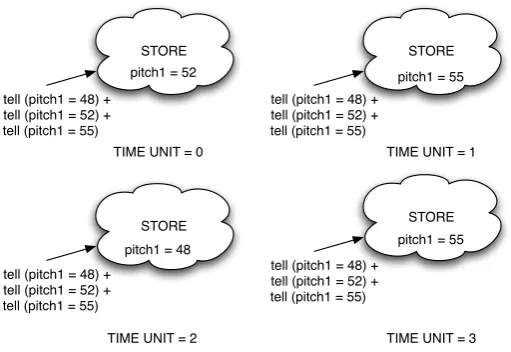
whentruedo tell(pitch=i) models a system where eachtime-unit, a note is chosen from the C major
chord (represented by the MIDI numbers 48,52 and 55) to be played (fig. 41).
The agents presented in table 2 are derived from the basic operators. The agent A + B non-deterministically chooses to execute eitherA orB. Thepersistent assignationprocess x←t changes the value ofxto the current value oftin the followingtime-units. In a similar way, the agents in table 3 are used to model cells. Cells are variables which value can be re-assigned in terms of its previous value.
x: (z) creates a new cellx with initial value z, x:←g(x) changes the value of a cell (this is different fromx←twhich changes the value of x only once), andexchg[x, y] exchanges the value of cellxandz. Finally, a basic recursion can be defined in ntcc with the form q(x) def= Pq, where q is the process name and Pq is restricted to call q at most once and such call must be within the scope of a “next”. The reason of using “next” is that we do not want an infinite recursion within atime-unit. Recursion is used to model iteration and recursive definitions. For instance, using this basic recursion, it is possible to write a function to compute the factorial function. Further information about recursion inntcc can
1 !P
i∈{48,52,55} whentruedo tell (pitch=i) can be expressed as !(tell(pitch = 48) +tell(pitch = 52) +tell
STORE
tell (pitch1 = 48) + tell (pitch1 = 52) + tell (pitch1 = 55)
STORE
tell (pitch1 = 48) + tell (pitch1 = 52) + tell (pitch1 = 55)
STORE
tell (pitch1 = 48) + tell (pitch1 = 52) + tell (pitch1 = 55)
STORE
tell (pitch1 = 48) + tell (pitch1 = 52) + tell (pitch1 = 55)
pitch1 = 52 pitch1 = 55
pitch1 = 48 pitch1 = 55 TIME UNIT = 0 TIME UNIT = 1
TIME UNIT = 2 TIME UNIT = 3
Figure 4: Execution of a non-deterministic process inntcc
Agent Meaning
A + B P
i∈1,2
when truedo(wheni= 1 doAkwhen i= 2do B )
x←t localv inP
v
when t=v do next!tell(x=v)
Table 2: Derivedntccagents
be found at [17].
2.3
Generic Constraint Development Environment (Gecode)
Gecode is a constraint solving library written in C++. Gecode is based on Constraints as Propagation agents (CPA) according to [39]. A CPA system provides multiple propagators to transform a (non-primitive) constraint into primitive constraints supplying the same information. In a finite domain constraint system, primitive constraints have the form x ∈ [a..b]. For instance, in a store containing
pitch1 ∈ [36..72], pitch2 ∈ [60..80], a propagator pitch1 > pitch2+ 2 would add constraints pitch1 ∈
[63..72] andpitch2∈[60..69].
The reader may notice that there is a similarity between CPA and ntcc. Both of them are based on concurrent agents working over a constraintstore. In chapter 6, we explain how we can encodentcc agents aspropagators.
Gecode works on different operating systems and is currently being used as the constraint library
for Alice[25] and soon it will be used in Mozart-Oz, therefore it will be maintained for a long time. Furthermore, it provides an extensible API, allowing us to create newpropagators. Finally, we conjecture
Agent Meaning
x: (z) tell(x=z)k unlesschange(x)nextx: (z)
x:←g(x) localv P
v
whenx=v do(tellchange(x)knextx:g(v) )
exchg[x, y] localv P
v
whent=v do(tell(change(x)k(tell(change(y)
knext(x:g(v)ky: (v))
that Gecode’s performance is better than the constraints solving tool-kits used in Sicstus Prolog and Mozart-Oz based on Gecode’s benchmarks2.
2.4
Factor Oracle (
FO
)
The Factor Oracle (FO)[1] is a finite automaton that can be built in linear time and space, in an incremental fashion. TheF Orecognizes at least all the sub-sequences (factors) of a given a sequence (it recognizes other sequences that are not factors). All the states of the F O are considered as accepting states. A sequence of symbols s = σ1σ2...σn is learned by such automaton, which states are 0,1,2...n. There is always a transition arrow (calledfactor link) from the statei−1 to the stateiand there are some transition arrows directed “backwards”, going from statei to j (wherei > j), calledsuffix links. Suffix
links, opposed tofactor links, are not labeled. For instance, aF O automaton for s = ab is presented in
Figure 5, where black headed arrows represent thefactor links and white headed arrows represent the
suffix links.
0 a 1 b 2
b
Figure 5: AF Oautomaton fors=ab
TheFO is built on-line and their authors proved that its algorithm has a linear complexity in time and space[1]. For each new entering symbol σ, a new state i is added and an arrow from i−1 toi is created with labelσi. Starting fromi−1, thesuffix links are iteratively followed backward, until a state is reached where afactor link with label σi going to some statej, or until there are no more suffix links to follow. For each state met during this iteration, a newfactor link labeled byσi is added from this state toi. Finally, a suffix link is added from i to statej or to state 0 depending on which condition terminated the iteration. Further formal definitions and the proof ofF Ocomplexity can be found in [1]. The on-line construction algorithm is presented with detail in Appendix??
Since theF O has a linear complexity in time and space, it was found in [10] that it is appropriate for machine improvisation. In addition, all attribute values for a music event can be kept in an object attached to the corresponding node, since the actual information structure is given by the configuration of arrows (factor and suffix links). Therefore a tuple withpitch(the frecuency of the note),duration(the amount of time that the note is played), andintensity (the volume on which is the note is played) can be related to each arrow according to [10].
2.5
Concurrent Constraint Factor Oracle Model for Music Improvisation
Concurrent Constraint Factor Oracle Model for Music Improvisation (Ccf omi) is defined in [28]. Follow-ing, we present a briefly explanation of the model taken from [28]. Ccf omihas three kinds of variables to represent the partially builtF Oautomaton: Variablesf romkare the set of labels of all currently existing f actor linksgoing forward fromk. VariablesSi are thesuffix links from each statei, and variableδk,σi give the state reached fromk by following af actor link labeledσi. For instance, the F Oin figure 5 is represented byf rom0={a, b},f rom1={b}, S1= 0,S2= 0,δ0,a= 1,δ0,b= 2.
Although it is not stated explicitly inCcf omi, the variablesf romk andδk,σi are modeled as infinite rational trees [24] with unary branching, allowing us to add elements to them, eachtime-unit. Infinite rational trees have infinite size. However, they only contain a finite number of distinct sub-trees. For that reason, they have been subjects of multiple axiomatizations to construct a constraint system based
on them. For instance, posting the constraintscons(c, nil, B),cons(b, B, C),cons(a, C, D) we can model a list of three elements [a, b, c].
Ccfomiis divided in three subsystems: learning (ADD), improvisation (CHOICE) and playing (PLAYER)
running concurrently. In addition, there is a synchronization process (SYNC) that takes care of synchro-nization.
TheADDprocess is in charge of building theF O(this process models the learning phase) by creating
thefactor links andsuffix links. Note that the processADD calls theLOOP process.
ADDi
def
= !tell(δi−1,σi =i)kLOOPi(Si−1)
“Process LOOPi(k) adds (if needed) factor links labeled σi to state i from all states k reached from i−1 bysuffix links, then computesSi, thesuffix link fromi” [28].
LOOPi(k) def
=
whenk≥0 do
unlessσi∈f romk
next(!tell(σi∈f romk)k!tell(δk,σi =i)kLOOPi(Sk))
kwhen k=−1 do!tell(Si= 0)
kwhen k≥0∧σi∈f romk do!tell(Si=δk,σi)
“A musician is modeled as a P LAY ER process playing some note p every once in a while. The
P LAY ER process non-deterministically chooses between playing a note now or postponing the decision to the nexttime-unit” [28].
P LAY ERj
def = P
p∈Σ
when truedo(!tell(σj=p)k tell(go=j)k nextP LAY ERj+1)
+ (tell(go=j−1)k nextP LAY ERj)
The learning and the simulation phase must work concurrently. In order to achieve that, it is required that the simulation phase only takes place once the sub-graph is completely built. TheSY N Ci process is in charge of doing the synchronization between the simulation and the learning phase to preserve that property.
Synchronizing both phases is greatly simplified by the used of constraints. When a variable has no value, thewhen processes depending on it are blocked. Therefore, theSY N Ci process is “waiting” until go is greater or equal than one. It means that the P LAY ERi process has played the note i and the ADDi process can add a new symbol to theF O. The other condition Si−1 ≥ −1 is because the first
suffix link of the FO is equal to -1 and it cannot be followed in the simulation phase.
SY N Ci def
=
whenSi−1≥ −1∧go≥ido(ADDi k nextSY N Ci+1)
k unlessSi−1≥ −1∧go≥inextSY N Ci)
“The improvisation processCHOICEΦ(k) uses the distribution function Φ : R→ {0,1}. The process
starts from statekand stochastically, chooses according to probability q, whether to output the symbol
σk or to follow a backward linkSk”[28].
CHOICEΦ(k)
def =
when Sk=−1do next(tell(out=σk+1)kCHOICEΦ(k+ 1))
ktell(f lip= Φk(q))
kwhenf lip= 1∧Sk+1≥0 do next(tell(out=σk+1)kCHOICEΦ(k+ 1))
next P
σ∈Σ
when σ∈f romsk do(tell (out=σ)k CHOICEΦ(δsk,σ)
The whole system is represented by a process doing all the initializations and launching the processes when corresponding. Improvisation starts afternsymbols have been created by theP LAY ER process.
Systemn,p def
=
!tell(q=p)k!tell(S0=−1)kP LAY ER1k SY N C1
k!when go=ndoCHOICE(n)
2.6
Probabilistic Non-deterministic Timed Concurrent Constraint (
pntcc
)
“One possible critique to CCP is that it is too generic for representing certain complex systems. Even if counting with partial information is extremely valuable, we find that properly taking into account certain phenomena remains to be difficult, which severely affects both modeling and verification. Particularly challenging is the case of uncertain behavior. Indeed, the uncertainty underlying concurrent interactions in areas such as computer music goes way beyond of what can be modeled using partial information only.” [20].
The first attempt to extend ntcc to work with probabilities was the Stochastic Non-deterministic
Timed Concurrent Constraint (sntcc[18])calculus. Sntccprovides an operatorPρ to decide whether to
execute or not a process with a certain probabilityρ. Usingsntcc,Ccfomimodels the action of choosing between asuffix link or afactor link with a probabilityρ. However, when usingsntcc, it is not possible to use a probability distribution to choose among all the factor links following a state in theFO. The probability distribution describes the range of possible values that a random variable can take.
Pntcc overcomes that problem, it provides a new agent to the calculus for probabilistic choice L. The probabilistic choiceLoperator has the following syntax:
L i∈I
when Ci do(Pi, ai),
whereI is a finite set of indexes, and for everyai∈R(0.0,1.0] we have P i∈I
ai = 1.0.
“The intuition of this operator is as follows. Each ai associated to Pi represents its probability of being selected for execution. Hence, the collection of all ai represents a probability distribution. The guards that can be entailed from the currentstore determine a subset of enabled processes, which are used to determine an eventual normalization of the ai’s. In the current time interval, the summation probabilistically chooses one of the enabled process according to the distribution defined by the (possibly normalized) ai0s. The chosen alternative, if any, precludes the others. If no choice is possible then the summation is precluded.” [20].
Using the probabilistic choice we can model a process choosing a factor link from the F O with a probability distributionρ.
L σ∈P
whenσ∈f romk do(tell(output=σ),ρσ)
The operational semantic of theLagent and other formal definitions aboutpntcc can be found in Appendix??.
3
Probabilistic Choice of Musical Sequences
In the beginning of this article, we developed a probabilistic model which changes the complexity in time for building the F O to quadratic (see Appendix ??). The idea behind it was changing the probabilities of all the factor links coming from statei when modifying afactor link leaving from that state. This idea was discarded for not being compatible with soft real-time (consider soft real-time as defined in the introduction).
The probabilistic model we chose is based on a simple, yet powerful concept. Using the system parameters, the probability of choosing a factor link in the simulation phase will decrease each time a
factor link is chosen. Additionally, we calculate the length of the common suffix (context) associated to
eachsuffix link. Using thecontext, we reward thesuffix links. Further information about thecontext can be found at [13].
We represent the system with four kind of variables used to represent: theFO states and transitions; the musical information attached to theFO; the probabilistic information; and the information to change musical attributes in the notes, based on the user style.
In addition to the variables described before, the system has some information parametrized by the user: α, β, γ, τ and n. The constant αis the recombination factor, representing the proportion of new sequences desired. βrepresents the factor for decreasing the importance of afactor link when it is chosen in the simulation phase. γ represents the importance of a new factor link in relation with the other
factor links coming from the same state. τ (described in Chapter 4) is a parameter for changing musical
attributes in the notes. Finally,nis a parameter representing the number of notes that must be learned before starting the simulation phase. In Chapter 5 we describe how can we use n to synchronize the improvisation phases.
We label eachfactor link by thepitch. Moreover, outside theF Odefinition, we create a tuple of three integers for eachfactor link: pitch,duration, andintensity. These three characteristics are represented by integers. The pitch and the intensity are represented by integers from 0 to 127 and the duration
is represented by milliseconds3. That way we can build apitch F O (i.e., a FO where the symbols are
pitches) associating to it other musical information.
At the same time we build a F O, we also create three integer arrays: ρ, C and sum. There is an
integerρi,σfor everyfactor link,Ci for everysuffix link, andsumi for every statei. Note thatρi,σ/sumi would represent the probability of choosing afactor link ifsuffix links were not considered, andCiis the
context.
Next, we show the learning and simulation phases for the probabilistic extension. We present some simple examples explaining how the probabilities are calculated in the learning phase and how they are used in the simulation phase. Finally, we present some concluding remarks and other improvisation models related to our model.
3.1
Stylistic learning phase
During the learning phase we store an integer ρi,σ for each factor link going fromi labelled by σ. We also store an integersumi for each stateiof the automaton.
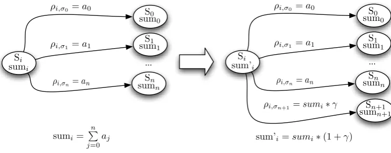
The initial value forρi,σissumi∗γ(fig. 6), whereγis a system parameter representing the importance of a new sequence in relation with the sequences already learned. When afactor link from ilabeled by
σj is the first factor link leaving fromi, we assign to sumi andρi,σj the constant c. We wantc to be a big integer, allowing us to have more precision when reasoning aboutρi,σj/sumi.
The reader may notice that this approach gives a certain importance to a newfactor link leaving from
i labeled byσj, without changing the value of all the other quantitiesρi,σ leaving fromi. Furthermore, we preserve the sum of all the values ρi,σ in the variable sumi, for each state i. This system exhibits a very important property: For each state i, P
σ∈f romi
[ρi,σ/sumi] = 1. The sum of all the probabilities
associated to the factor links coming from the same state are equal to one. This property is preserved, when changing the values ofρi,σ andsumi in both improvisation phases.
On the other hand, we give rewards to the suffix link using the context. To calculate the context, Lefebvre and Lecroq modified theF Oconstruction algorithm, conserving its linear complexity in time and
... sum0
sum1
S0
S1
Si
ρi,σ0 =a0
ρi,σ1 =a1
ρi,σn=an
ρi,σn+1 =sumi∗γ
... sumi
sum0
sum1
S0
S1
Si
ρi,σ0=a0
ρi,σ1=a1
ρi,σn=an
sumi= n ! j=0
aj
sum’i Sn
sumn
sum’i=sumi∗(1 +γ)
sumn+1
Sn+1
Sn sumn
Figure 6: Adding afactor link to theFO
space [13]. This approach has been successfully used by Cont, Assayag and Dubnov on their anticipatory improvisation model [7].
Figure 7 is a simple example of aFO and the integer arrays presented previously. First, we present the score of a fragment of the Happy Birthday song; then we present a sequence of possible tuples< pitch,
duration,intensity >for that fragment; and finally theFO with the probabilistic information.
3.2
Stylistic simulation phase
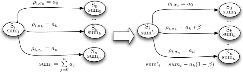
In the simulation phase, we use all the information calculated in the learning phase to choose the notes probabilistically. Factor links chosen in this phase, will decrease the importance proportionally toβ. In addition, the probability of choosing secondaryfactor links is proportional to γ . We consider primary
factor links those going from the state ito i+ 1, and all the others as secondary . On the other hand,
thesuffix links are rewarded by thecontext, calculated on-line in the learning phase.
If there were notsuffix links, we would choose afactor link leaving from the stateiwith a probability distribution ϕ(i, σ) such that ϕ(i, σ) = ρi,σ/sumi. Later on, we will explain how we can extend this concept to work with thesuffix links, rewarded by theircontext. However, the concept of decreasing the probability of afactor link when it is chosen remains invariant.
When the system chooses a certain factor link leaving from i and labeled byσk, the value of ρi,σ is decremented, multiplying it by β. Subsequently, we update the new value of sumi by subtracting (1−β)∗ai,σk (fig. 8). That way, we preserve the property
P σ∈f romi
[ρi,σ/sumi] = 1 for each statei. Note
that we are only adding constant time operations, making our model compatible with soft real-time. Following only thefactor links we obtain all the factor (subsequences) of the original sequence. This causes two problems: first, if we always follow thefactor links, soon we will get to the last state of the automaton; second, we only improvise over the subsequences of the information learned from the user, without sequence variation. This would make the improvisation repetitive. Following thesuffix link we achieve sequence variation because we can combine different suffixes and prefixes of the sequences learned. For instance, inOmax[3] –a model for music improvisation processing in real-time audio and video– this is called recombination and it is parametrized by a recombination factor.
Rueda et al approaches this problem inCcf omiby creating a probability distribution parameterized by a valueα. The probability of choosing afactor link is given byαand the probability of choosing a
suffix link is given by 1−α. There is a drawback in this approach. Since it does not reward thesuffix
linkswith thecontext (the length of the common suffix), this system may choose multiple times in a row
suffix links going back one or two states, creating repetitive sequences.
4
3
Music engraving by LilyPond 2.11.31—www.lilypond.org
(a) The Score of the fragment
(G, 375,80), (G, 125,60), (A, 500,100), (G, 500,90), (C, 500,100), (B, 1000,60) (b) Fragment of the Happy Birthday Song represented with tuples
S0 S1 S2 S3 S4 S5 S6 (C,500,100) (B,1000,60) (G,125,60) (A,500,100) (A,500,100) (A,500,100) (G,500,90) (C,500,100) (C,500,100) (B,1000,60) C1 C2 C3 C4 C5 C6 ρ 0,G
ρ1,A
ρ0,A
ρ3,G
ρ0,C
ρ4,C
ρ1,C
ρ5,B
ρ0,B
ρ1,G
sum1 sum0 sum3 sum4 sum5 sum6 sum2
ρ2,A (G,
375 ,80)
(c) Factor Oracle with the probabilistic information
Figure 7: Factor Oracle used to represent a Happy Birthday fragment
...
sumi
sum0
S0
Si
ρi,σ0 =a0
sumi= n ! j=0 aj ... Sk sumk ρi,σk=ak
...
sum0
S0
Si
ρi,σ0=a0
...
Sk sumk ρi,σk=ak∗β
ρi,σn =an ρi,σ
n =an
sum’i=sumi−ak(1−β) sum’i
sumn Sn Sn
sumn
Figure 8: Choosing afactor link fromklabelled byσk
ϕ(S(i), σ) =ρS(i),σ/sumS(i) and no way to relate them. Using thecontext Ci, we create a probability distribution Φ(i, σ) ranking thefactor links leaving from the stateS(i) with the productα∗C(i).
Φ(i, σ) = ( ρi,σ
sumi ifS(i) =−1,
ρi,σ+ρS(i),σ∗Ci∗α
sumi+sumS(i)∗Ci∗α ifS(i)>−1
Using Φ(i, σ), the system is able to choose a symbol at any state of theF O. The advantage of this probability distribution over the one presented in Ccf omi, is that it takes into account the context, as well as the recombination factorα.
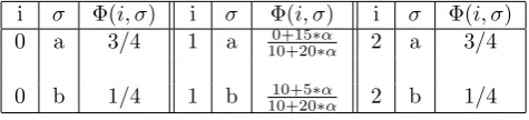
To exemplify how to build this probability distribution, consider theF Owith the probabilistic infor-mation in figure 9. That example correspond to theF O for s= ab and random values for the integer arrays described in this chapter. Table 4 shows how to build a probability distribution Φ(i, σ) for the
F Oin figure 9.
Note that for the states zero and two in the table, the probabilities calculated are the same. This happens because the first state does not have asuffix link to go backwards and the last state does not
havefactor links to go forward. On the other hand, the probabilities calculated for the state one combine
the probability of choosing afactor link following state 1 or choosing thesuffix link and then choosing a
factor link from state zero.
S0 S1 S2
sum0= 20 sum1= 10 sum2= 0
A
B
ρ0,A= 15
ρ0,B = 5
ρ1,B = 10
C1= 1 C2= 2
B
Figure 9: A Factor Oracle including probabilities, for the sequences=ab
i σ Φ(i, σ) i σ Φ(i, σ) i σ Φ(i, σ) 0 a 3/4 1 a 10+200+15∗∗αα 2 a 3/4
0 b 1/4 1 b 10+2010+5∗∗αα 2 b 1/4
Table 4: Probability distribution Φ(i, σ) for figure 9
3.3
Summary
In this chapter we explained how we can model music improvisation using probabilities, extending the notion of non-deterministic choice described inCcf omi. The intuition is decreasing the probability of choosing afactor link, each time it is chosen and rewarding asuffix link based on thecontext. Further-more, we explained how the parametersα, β, and γ allow us to parameterize the computation of the probabilities.
This procedure is simple enough so that the probabilities can be computed in constant time when the
F Ois built, preserving the linear complexity in time and space of theF Oon-line construction algorithm. Additionally, using probabilities allows us to generate different sequences, without repeating the same sequence multiple times in a row likeCcf omi.
3.4
Related work
produces more “interesting” sequences.
There is an extension ofCcf omiusingpntcc. The use ofpntccmakes possible to choose the sequences in the simulation phase, based on a probability distribution. Although Perez and Rueda modeled the probabilistic choice of sequences using theF O, they do not provide a description of how those probabilities can be calculated during the learning phase.
4
Changing Musical Attributes of the Notes
According to Conklin [4], music-generation systems aim to create music based on some predefined rules and a corpus (i.e., a collection of musical pieces in a certain music style) learned previously. Those systems can create new musical material based on the style of thecorpus learned. Unfortunately, they use algorithms with high complexity in time and space, making them inappropriate for music interaction according to [10]. On the other hand, interactive systems for music improvisation (e.g., Ccf omi) are usually based on the recombination of sequences learned from the user.
Although recombination creates new sequences based on the user style, it does not create new notes. In fact, it does not even change a single characteristic of a note. To solve that problem, one of the objectives of this article is changing at least one musical attribute of the notes generated during the style simulation.
In the beginning of this work, we tried to develop an algorithm for creating new notes, based on the learned style. The idea was calculating the probability of being on a certain music scale. Based on that probability, we choose a random pitch from that scale. A music scale is an ascending or descending series of notes or pitches. We also developed an algorithm to calculate the duration of those new notes (see Appendix??).
We did not include those ideas in this article. First, because choosing apitchbased on a supposition of the scale cannot be generalized to music which is not based on scales. In addition, because the procedure for calculating the probability of being on a certain scale was not very accurate, as we found out during some tests. Finally, because the algorithm to generate new durations is not compatible with soft real-time. The approach we chose to change a musical attribute is again based on simple, but powerful concept. We store the averageintensity(the other musical attributes are not changed in our model for the reasons mentioned above) of the notes currently being played (current dynamics) by the computer. We also store
the current dynamics of the user. Then, we compare them and change the current dynamics of the
computer (if necessary), making it similar to the usercurrent dynamics. The idea behind thisintensity
variation was originally proposed by musicians Riascos and Collazos . It is based on a concept that they usually apply when improvising with other musicians.
In order to formalize that concept, we calculate, in the learning phase, thecurrent dynamics of the last τ (a system parameter) notes played by both, the user and the computer, separately. Concurrently, in the simulation phase, we compare the two current dynamics. If they are not equal, we multiply the intensity of the current note being played by the computer by a factor proportional to relation of the user and computercurrent dynamics. As follows, we explain in detail how we can calculate thecurrent
dynamics in the learning phase and how to change theintensityof notes generated in simulation phase.
4.1
Stylistic learning phase
Theintensityin music represents two different things at the same time. When analyzing theintensityof a single note in a sequence, we reason about thatintensity as a musical accent meaning the importance of certain notes or defining rhythms. On the other hand, we reason about the average intensity of a sequence of notes as the dynamics of that sequence of notes. The accents may be written explicitly in the score with a symbol> bellow the note and the dynamics for relative loudness may be written explicitly in the score as piano (p), forte (f), fortissimo (f f), etc.
To capture these two concepts, in the learning phase we store the intensity in a tuple < pitch,
duration,intensity >. In addition, we store thecurrent dynamicsfor the lastτ notes played by the user
Qu and the computerQc.
intensities I, the value forτ, a reference to the queue Qi, and thecurrent dynamic Qi. The invariant of the algorithm is always having the average of the queue data in the variableQi and the sum in the variableIntensitySum. Append??gives an example of the operation of this algorithm.
CALCULATE-CURRENT-DYNAMICS(I=I1I2...Im,τ, Qi,Qi)
01 Qi ←new Queue(τ)
02 IntensitySum←0
03 QueueSize←0 04 fori←0to mdo
05 if QueueSize < τ then
06 IntensitySum←IntensitySum+Ii
07 else IntensitySum←IntensitySum+Ii -Qi.pop()
08 Qi.push(Ii)
09 Qi ←IntensitySum/QueueSize
4.2
Stylistic simulation phase
In this phase, we traverse the F O using the probabilistic distribution Φ(i, σ) proposed in chapter 3. Remember that there is anintensity and adurationassociated to eachpitch in theF O. If we play the
intensitieswith the same value as they were learned, we could have a problem of coherence between the
current dynamics of the user and thecurrent dynamics of the sequences we are producing.
To give an example of this problem, consider the Happy Birthday fragment presented in figure 7. The
current dynamics for that fragment is 98. Now, suppose the computer current dynamics is 30. This
poses a problem, because the user is expecting the computer to improvise in the samedynamics that he is, according to the interviews with Riascos and Collazos.
The solution we propose is multiplying by a factor Qc/Qu the intensity of every note generated by the computer. In the previous example, the next note generated by the computer would be multiplied by a factor of 30/98.
4.3
Summary
We explained how we can change theintensityof the notes generated during the improvisation. The idea is to maintain thecurrent dynamics of the notes generated by the computer similar thecurrent dynamics
of the notes generated by the user. This corresponds to formalizing an improvisation technique used by two musicians interviewed for this article.
This kind of variation in theintensityis something new for machine improvisation systems as far as we know. We believe that this kind of approach, where simple variations can be made preserving the style learned from the user and being compatible with real-time, should be a topic of investigation in future works.
4.4
Related work
NeitherCcf omi nor its probabilistic extension provides a way to change musical attributes of the notes nor creating new material based on the user style.
5
Modeling the system in
pntcc
Ntcchas been used in a large variety of situations for synchronizing musical processes. From the introduc-tion chapter, we recall the models for interactive scores, audio processing, formalizing musical processes, and music improvisation. In those models, the synchronization is made declaratively. It means thatntcc hides the details on how the processes are synchronized and how the shared resources (in thestore) are accessed.
One objective of this work is modeling our improvisation system withntcc. So far, we presented the modifications for the improvisation phases allowing probabilistic choice of musical sequences and changing the musical attributes in the simulation phase. Since we are choosing the sequences probabilistically, we usepntcc(the probabilistic extension of ntcc) for modeling our improvisation system.
In order to synchronize the improvisation phases, the learning phase must take place from the begin-ning. However, the simulation phase is launched once the learning phase has learnednnotes. After that, both phases run concurrently. Synchronization must be provided because the improvisation phase must not work in partially built graphs, it can only improvise in the fragment of the graph that represents a
F O. Additionally, the simulation phase can only work in statekonce the value for thecurrent dynamics, thecontext, and theprobabilistic distribution has been calculated up to statek.
Our approach to synchronize the improvisation phases is similar to the one used inCcfomi. Remem-ber that Ccfomi synchronizes the improvisation phases using a variable go and the variables Si. The P LAY ERprocess can post constraints over those variables and the processes for building theF O(ADD
and LOOP) are activated when they can deduce certain information from those variables. We extend that concept using some of the new variables introduced in this model.
In addition to the variablesf romk,Si, andδi,σ used inCcf omi, our model has a few more variables: ρi,σ,sumi, Φi,σ, andCirepresent the probabilistic choice of musical sequences;durationσandintensityσ represent the musical attributes associated to each pitchσ; andQi,SumQiandQirepresent the intensity variation. The variables Φi,σ, Ci, Qi, durationσ, and intensityσ are represented with rational trees of F D variables because they do not change their value from a time-unit to another. The other variables are represented with cells (cells are defined in chapter 2).
In this chapter, we explain how we can write a sequential algorithm for the learning phase combining the algorithm for building on-line theF O, calculating thecontext, calculating the probabilistic distribu-tion Φk,σ and the current dynamics. After that, we show how both phases can be modeled in pntcc. Finally, we give some concluding remarks and we present related work.
5.1
Modeling the stylistic learning phase
The learning phase can be easily integrated to the on-line algorithm that builds a F O and calculates
the context (the original algorithms are presented in Appendix ??). The learning phase is
repre-sented by the functions Ext Oracle On-line and Ext Add Letter. To calculate the context we use the
Length Repeated Suffix function proposed by Lefevre et al. The Length Repeated Suffix calculates the
context. It finds the length of a repeated suffix ofP[1..i+ 1] in linear time and space complexity.
TheExt Add Letter function is in charge of adding new pitches to the F O. It also creates a tuple
< pitch, duration, intensity >; updates values ofρi,σ andsumi; and calculates thecurrent dynamics of the userQu, and thecontext Ci+1for statei+ 1. This function receives aF Owithistates, a pitchσ, the
duration, the intensity, the system parametersγandτ, and the Intensity QueueQi. During its execution, it uses the constantc, the functionS(i), and the temporal variable π. C is a big integer constant,S(i) is a function returning thesuffix link for statei, andπis a temporal variable used to calculate thecontext.
EXT ADD LETTER(Oracle(P[1..i]),σ,duration,intensity,γ,τ,Qi) 01 Create a new statei+ 1
04 π1←i
05 ρi,σ←c 06 sumi←c
07 if QueueSize < τ then
08 intensitySum←IntensitySum+intensity
09 elseIntensitySum←intensity -Qi.pop()
10 Qi.push(Ii)
11 Qi ←IntensitySum/QueueSize
12 durationσ←duration
13 intensityσ ←intensity
14 Whilek >−1 andδ(k, σ) is undefineddo
15 δ(k, σ)←i+ 1 16 π1←k
17 k←S(k) 18 ρk,σ ←sumk∗γ 19 sumk ←sumk∗(1 +γ) 20 if k=−1 thenS(i+ 1)←0 21 elseS(i+ 1)←δ(k, σ)
22 Ci+1←LEN GT H REP EAT ED SU F F IX(π1, S(i+ 1))
23 ReturnOracle(P[1..i]σ)
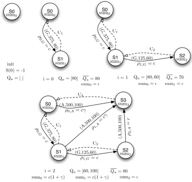
TheExt Oracle On-line function is a sequential algorithm representing the learning phase. It receives
three vectors: the pitches, the durations, and the intensities. In addition, it takesγ, the system parameter for ranking the importance of a new note added to theF O, and the system parameterτ, representing the number of notes taken into account to calculate thecurrent dynamics. Figure 10 presents the execution of this function for the three first symbols of the Happy Birthday Fragment presented in figure 7.
EXT ORACLE ON LINE(P[1..m],D[1..m],I[1..m],γ,τ) 01 Create Oracle() with one single state 0 andS(0) =−1
02 Qu ←new Queue(τ)
03 IntensitySum←0
04 fori←1to mdoOracle([1..i])←
05 EXT ADD LETTER(Oracle(P[1..i−1]),Pi,Di,Ii,γ,τ,Qu)
The learning phase is modeled inpntcc by the processes P HI,ADD, LOOP, ADD ELEM EN T,
P LAY ER,CON T EXT, andCON T EXT LOOP. ProcessP HI calculates the values for the
probabil-ity distributionφk,σ, used to choose Afactor link leaving from stateklabeled by a symbolσ. Where the recombination factor is parameterized byα. The process T ree| represents the act of adding a “fresh” variable to the infinite rational tree (as described in chapter 2). We use infinite rational trees to represent the variable such asf romandδthat represents the transitions of the F O.
P HI(k, σ, α)def=
whenSk=−1do!tell(φk,σ= sumρk,σk) kwhenSk >−1do !tell(φk,σ=
ρi,σ+ρS(i),σ∗Ci∗α sumi+sumS(i)∗Ci∗α)k φ|
The ProcessADD is the one in charge of adding new pitches to the F O. In addition, this process updates the values of the cellsρand the variableφcalling the functionP HI.
ADDi(α, γ) def
=
δi−1,σi←i k!tell(σi∈f romi−1)k ρi−1,σi: (c)k sumi−1: (c)
k P HI(i−1, σi, α)kf rom| kδ| kρ| ksum| knextLOOPi(Si−1, α, γ, i−1)
TheLOOP process represents the “while” loop in the Ext Add Letter function. This process adds a
S0 S1 S2 S3 (G,125,60) (A,500,100) (A,500,100) (A,500,100) C1 C2 C3 ρ0 ,G = c
ρ1,A
=cγ ρ0,A=cγ
ρ1,G =c sum1
sum0 sum3
sum2
ρ,A2
= c (G, 375 ,80) S0
S1 (G,125,60) S2
C1 C2 ρ0 ,G = c
ρ1,G =c sum1 sum0 sum2 (G, 375 ,80) S0 S1 C1 ρ0 ,G = c sum1 sum0 (G, 375 ,80) S0 sum0
i = 0 i = 1
i = 2 init
Qu= [80] Qu= [80,60]
Qu= [60,100]
Qu= 80 Qu= 70
Qu= 80 Qu= [ ]
S(0) = -1
sum0=c sum0=c sum1=c
sum2=c
sum0=c(1 +γ) sum1=c(1 +γ)
Figure 10: Executing theExt Oracle On-line algorithm withτ = 2
transition from k labeled byσ. The values fork depends on thesuffix links. In addition, it calculates the values for thecontext Ci and the probabilistic information.
LOOPi(k, α, γ, π1)
def =
whenk≥0 do(
whenσi∈f romk do
(!tell(Si=δk,σi)kS| kCON T EXT(i, π1, Si) )
kunlessσi ∈f romk next (
sumk :←sumk(1 +γ)ksum| ||ρk,σi :←γsumk k ρ| kP HI(α, k, σi)
||next( !tell(σi ∈f romk)|| !tell(δk,σi =i)
|| LOOPi(Sk, α, γ, k)kf rom| kδ|)))
kwhen k=−1 do( !tell(Si= 0)k S| kCON T EXT(i, π1, Si) )
In the CON T EXT process the reader may notice how we can use when a 6= b do P instead of
unless a 6=b next P because we know that a,b always have a value. The values π, s, π1 andpi2 are
used to calculate efficiently thecontext according to Lefevre et al.’s algorithm.
whens= 0do!tell(Ci= 0) kwhens6= 0do(
whens−1 =Sπ1do!tell (Ci=Cπ1+ 1)
kwhen s−16=Sπ1 doCON T EXT LOOP(π, s−1, i))
CON T EXT LOOP(π1, π2, i)
def =
whenSπ1=Sπ2 do!tell(Ci=min(Cπ1,Cπ2) + 1)
kwhenSπ1 6=Sπ2 do next CON T EXT LOOP(π1, Sπ2, i)
TheADD ELEM EN T process calculates the value for thecurrent dynamics. In addition, it updates
sumbased on the parameterτ.
ADD ELEM EN T(Q, I, τ, index, sum, Q)def=
whenindex≥τ dosum:←sum+I−Qindex−τ
kwhenindex < τ do sum:←sum+I kQ:←sum/min(index, τ)
Finally, theP LAY ER stores the values ofpitch,duration, andintensity received from the environ-ment when a note is played by the user. Furthermore, it updates thecurrent dynamics Qu.
P LAY ERj
def =
whenP >0∧D >0∧I >0do(
ADD ELEM EN T(Qu, I, τ, j, SumQu, Qu) knext ( !tell(σj=P)kQu| k!tellQuj =I
k!tell(durationσj =D)k !tell(intensityσj =I)ktell(go=i)k P LAY ERj+1))
kunlessP >0∧D >0∧I >0next (tell(go=j−1) kP LAY ERj )
5.2
Modeling the style simulation phase
In this phase, we use the L agent, defined in pntcc to model probabilistic choice. This model is an extension of the model presented in [20]. In our model, theIM P ROV process chooses a link according to the probability distribution φk,σi. Furthermore, it updates the values for sum and ρ, sets-up the outputs, and updates the computercurrent dynamics Qc.
In order to ask if a constraintA∧B orA∨B can be deduced from thestore, we use reification. For instance, the processwhen a=b∧c =ddo P, can be codified as the process when g doP and the constraintsa=b↔e,c=d↔f,e∧f ↔g.
IM P ROV(k, τ, β)def=
||whenL Ck ≥0do(
i∈P
when σi∈f romk∨σi ∈f romSk do(
next(tell (out pitch=σi)|| tell(out duration=durationσi)
|| tell(out intensity=intensityσi∗Qu/Qc)|| tell(Qci=intensityσi)
|| ADD ELEM EN T(Qc, out intensity, τ, i, SumQc, Qc))
|| whenσi∈f romk∧σi∈f romSk do next(IM P ROV(k+ 1, τ, β) +IM P ROV(Sk, τ, β))
|| unlessσi∈f romk next(IM P ROV(Sk, τ, β)
|| ρSk,σi:←β∗ρSk,σi || sumSk:←sumSk−(1−β)ρSk,σi )
|| unlessσi∈f romSk next(IM P ROV(k+ 1, τ, β)
|| ρk,σi :←β∗ρk,σi ||sumk:←sumk−(1−β)ρk,σi),Φk,σi)
||unless Ck ≥0nextIM P ROV(k, τ, β)
5.3
Synchronizing the improvisation phases
Synchronizing both phases is greatly simplified by the used of constraints. When a variable has no value,
greater or equal than one. That means that theP LAY ERi process has played the noteiand theADDi process can add a new symbol to the FO. The other conditionSi−1≥ −1 is because the firstsuffix link
of the FO is equal -1 and that suffix link cannot be followed in the simulation phase. In addition, the
SY N C process is also “waiting” for thecurrent dynamics Qu to take a value greater of equal than 0.
SY N Ci(α, γ) def
=
whenSi−1≥ −1∧go≥i∧Qu>0 do(ADDi(α, γ)k nextSY N Ci+1(α, γ))
||unless Si−1≥ −1∧go≥i∧Qu>0nextSY N Ci(α, γ)
A waitn process is necessary to wait until n symbols have been learned to launch the IM P ROV process.
W AIT(n, τ, β)def=
whengo=ndo nextIM P ROV(n, τ, β)|| unlessgo=nnextW AIT(n, τ, β)
The system is modeled as the P LAY ER and the SY N C process running in parallel with a process waiting until n symbols have been played to start theIM P ROV process. The reader should remeber that α is the recombination factor, representing the proportion of new sequences desired. β represents the factor for decreasing the importance of a factor link when it is chosen in the simulation phase. γ
represents the importance of a new factor link in relation with the other factor links coming from the same state. τ is a parameter for changing musical attributes in the notes. Finally, n is a parameter representing the number of notes that must be learned before starting the simulation phase.
SY ST EM(n, α, β, γ, τ)def=
!tell(S0=−1)|| SY N C1(α, γ)||P LAY ER1(τ)|| W AIT(n, τ, β)
5.4
Summary
We modeled all the concepts described in previous chapters usingpntcc. Although synchronization and probabilistic choice are modeled declaratively, matching the time-units is not an easy task because the value of a cell only can be changed in the followingtime-unit. If we change the value of a cell in the scope of anunless process, we need to be aware that the value will only be changed twotime-units after.
5.5
Related work
The Omax model uses F O, but instead of using ntcc, it uses shared state concurrency (for synchro-nizing the improvisation phases) and message passing concurrency (for synchrosynchro-nizing OpenMusic and Max/Msp). Although this a remarkable model, we believe that ntcc can provide an easier way to syn-chronize processes and to reason about the correctness of the implementation because it is obviously easier to synchronize declaratively. Constraints provide a much more powerful way to express declara-tively complex synchronizing patterns. Since thentccmodel has a logical counterpart [17], it is possible to prove properties of the model. For instance, the fact that it always (or never or sometimes) chooses the longest context, or that repetitions of some given subsequence are avoided.
Probabilistic Ccofmi [20] fixes the problems with synchronization and extends the notion of
proba-bilistic choice in the improvisation phase, giving it a clear and concise semantic. However, it does not model how can probabilistic distributions may change from a time-unit to another based on user and computer interaction.
6
Implementation
are designed to simulate a finite ntcc model. It means that they only simulate a finite number of
time-units.
During the last decade, three interpreters for ntcc have been developed. Lman [16] by Hurtado and Mu˜noz in 2003, NtccSim (http://avispa.puj.edu.co) by the Avispa research group in 2006, and
Rueda’s sim in 2006. They were intended to simulatentccmodels, but they were not made for real-time
interaction. Recall from the introduction that soft real-time interaction means that the user does not experience noticeable delays in the interaction.
When designing a ntcc interpreter, we need a constraint solving library or programming language allowing us to check stability (i.e., know when a time-unit is over), check entailment (i.e., know if a constraint can be deduced from thestore), post constraints, and synchronize the concurrent access to the
store. These tasks must be performed efficiently to achieve a good performance.
The authors of thentcc model for interactive scores proposed to use Gecode as a constraint solving library for futurentcc interpreters, and create an interface for Gecode to OpenMusic to specify multi-media interaction applications. Furthermore, they proposed to extendLman to work under Mac OS X using Gecode.
One objective of this article is to develop a prototype for a ntcc interpreter real-time capable. We followed the advise from the authors of the interactive scores model and we tried out several alternatives to develop an interpreter using Gecode.
Our first attempt was using a thread to represent each ntcc process in the simulation. However, we found out that using threads adds an overhead in the performance of the interpreter because of the context-switch among threads, even when using lightweight (lw) threads. Then, we tried using event-driven programming. Performance was better compared with threaded implementations. However, each time awhen process asks if a condition can be entailed, we need to check for stability, thus adding an unnecessary overhead. The reader may find more information about our previous attempts in Appendix
??and performance results in chapter 7.
Our implementation,Ntccrt, is once again based on a simple but powerful concept. ThewhenandP processes are encoded as propagators in Gecode. That way Gecode manages all the concurrency required for the interpreter. Gecode calls the continuation of a process when a process condition is assigned to true.
On the other hand, tell processes are trivially codified to existing Gecode propagators and timed agents (i.e. ∗, !,unless,←andnext) are managed providing different process queues for eachtime-unit
in the simulation.
Our interpreter works in two modes, the developing mode and the interaction mode. In the developing mode, the users may specify the ntcc system that they want to simulate in the interpreter. In the interaction mode, the users execute the models and interact with them.
This chapter is about the design and implementation of Ntccrt. We explain how to encode all the ntccprocesses. We also explain the execution model of the interpreter. After that, we show how to run
Ccfomi in the interpreter.
In addition, we describe how we made an interface to OpenMusic and how we can generate binary plugins for data-flow programming languages: Pure Data (Pd) [22] or Max/Msp [23] where MIDI, audio, or video inputs/outputs can interact with aNtccrt binary. Finally, we give some conclusions, future work, and a short description of the other existing interpreters. A detailed description ofNtccrt, the generation of binary plugins, Pure Data, Max/Msp, and the previousNtccrt prototypes can be found in a previous publication [35].
6.1
Design of
Ntccrt
Our first version ofNtccrt allowed us to specify ntccmodels in C++ and execute them as stand-alone programs. Current version offers the possibility to specify a ntcc model on either Lisp, Openmusic or C++. In addition, currently, it is possible to execute ntcc models as a stand-alone program or as an
6.1.1 Developing mode
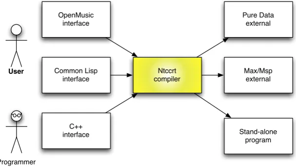
In order to write antccmodel inNtccrt, the user may write it directly in C++, use a parser that takes Common Lisp macros as input or defining a graphical “patch” in OpenMusic. Using either of these representations, it is possible to generate a stand-alone program or anexternal object (fig 11).
OpenMusic interface
Ntccrt compiler
Pure Data external
Max/Msp external Common Lisp
interface
C++
interface Stand-alone
program User
Programmer
Figure 11: Ntccrt: Developing mode
To make an interface for OpenMusic, first, we developed a Lisp parser using Common Lisp macros to write anntccmodel in Lisp syntax and translate it to C++ code. Lisp macros extend Lisp syntax to give special meaning to characters reserved for users for this purpose. Executing those macros automatically compile a ntccprogram.
After the success with Lisp macros, we created OpenMusic methods to represent ntcc processes. Openmusic methods are a graphical representation using the Common Lisp Object System (CLOS). Those graphical objects are placed on a graphical “patch”. Executing the “patch” generates a Ntccrt
C++ program.
6.1.2 Execution mode
To execute aNtccrt program we can proceed in two different ways. We can create a stand-alone program that can interact with the Midishare library [8], or we can create an external object for either Pd or Max. An advantage of compiling a ntcc model as an external object lies in using control signals and the message passing API provided by Pd and Max to synchronize any graphical object with theNtccrt
external.
To handle MIDI streams (e.g., MIDI files, MIDI instruments, or MIDI streams from other programs) we use the predefined functions in Pd or Max to process MIDI. Then, we connect the output of those functions to the Ntccrt binary plugin. We also provide an interface for Midishare, useful when running stand-alone programs (fig. 12).
6.2
Implementation of
Ntccrt
Ntccrt is the firstntccinterpreter written in C++ using Gecode. In this section, we focus on describing
Ntccrt Program Midishare input
Midi input
Control signals
Midishare output
Midi output
Control signals
Only Available when executing a Ntccrt program in Pure Data or Max/Msp
Figure 12: Ntccrt: Interaction mode
6.2.1 Data structures
To represent the constraint systems we need to provide new data types. Gecode variables work on a particularstore. Therefore, we need an abstraction to representntccvariables present on multiplestores
with the same variable object. Boolean variables are represented by theBoolV class, FD variables by the IntV class, FS variables by the SetV class, and infinite rational trees (with unary branching) by
SetV Array, BoolV Array, andIntV Array classes.
After encoding the constraint systems, we defined a way to represent each process. All of them are classes inheriting fromAskBody. AskBody is a class, defining anExecutemethod, which can be called by another object when it is nested on it.
To represent the tell agent, we defined a super class T ell. For this prototype, we provide three subclasses to represent these processes: tell (a=b), tell(a∈B), andtell(a > b). Other kind of tell
agents can be easily defined by inheriting from theT ellsuperclass and declaring an Executemethod. For the when agent, we made a When propagator and a When class for calling the propagator. A processwhen CdoP is represented by two propagators: C↔b(a reified propagator for the constraint
C) and if b thenP else skip(theWhen propagator). The When propagator checks the value of b. If the value ofb is true, it calls the Execute method ofP. Otherwise, it does not take any action. Figure 13 shows how to encode the processwhen a=c doP using theWhen propagator
whena=cdoP
STORE STORE
a=c↔b
b
ifbthenP
elseskip
Figure 13: Example of theWhen propagator

![Gestao de beneficios na etapa de projecto em empreendimentos hospitalares do reino unido [Managing benefits in the design of healthcare favilities in the UK]](data:image/gif;base64,R0lGODlhAQABAIAAAP///wAAACH5BAEAAAAALAAAAAABAAEAAAICRAEAOw==)