Correction of the significance level when attempting multiple transformations of an explanatory variable in generalized linear models

R E S E A R C H A R T I C L E

Open Access

Correction of the significance level when

attempting multiple transformations of an

explanatory variable in generalized linear

models

Benoit Liquet

and Jérémie Riou

Abstract

Background: In statistical modeling, finding the most favorable coding for an exploratory quantitative variable involves many tests. This process involves multiple testing problems and requires the correction of the significance level.

Methods: For each coding, a test on the nullity of the coefficient associated with the new coded variable is computed. The selected coding corresponds to that associated with the largest statistical test (or equivalently the smallestpvalue). In the context of the Generalized Linear Model, Liquet and Commenges (Stat Probability

Lett,71:33–38,2005) proposed an asymptotic correction of the significance level. This procedure, based on the score test, has been developed for dichotomous and Box-Cox transformations. In this paper, we suggest the use of resampling methods to estimate the significance level for categorical transformations with more than two levels and, by definition those that involve more than one parameter in the model. The categorical transformation is a more flexible way to explore the unknown shape of the effect between an explanatory and a dependent variable.

Results: The simulations we ran in this study showed good performances of the proposed methods. These methods were illustrated using the data from a study of the relationship between cholesterol and dementia.

Conclusion: The algorithms were implemented using R, and the associated CPMCGLM R package is available on the CRAN.

Keywords: Bonferroni procedure, Generalized linear model, Multiple coding, Parametric bootstrap, Permutation,

pvalue, Resampling procedure

Background

In applied studies, the relationship between an explana-tory and a dependent variable is routinely measured using a statistical model. For instance, in epidemiology it is quite common that a study focuses on one particular risk factor. The scientific problem is to analyze whether this risk fac-tor has an influence on the risk of occurrence of a disease, a biological trait , or another outcome. To answer to this

*Correspondence: [email protected]

1University Bordeaux, ISPED, Centre INSERM U-897-Epidemiologie-Biostatistique, Bordeaux, F-33000, France

2INSERM, ISPED, Centre INSERM U-897-Epidemiologie-Biostatistique, Bordeaux, F-33000, France

Full list of author information is available at the end of the article

question, a regression model is often used in which the risk factor will be represented by a continuousX, allow-ing adjustment onp−1 known risk factors of the studied trait. However, the form of the effect (or the dose-effect relationship) is not known in advance, and as such, the continuous variableXis often transformed, typically into categorical variables, by grouping values into two or more categories. An example of this is seen in anThe American Journal of Epidemiology(October 2009, volume 170, num-ber 8), where four of six papers with continuous exposure used categorization, and only two kept the variable as continuous [1].

Binary coding is often used in epidemiology, either to make interpretation easier, or because a threshold effect is suspected. In a regression model with multiple explana-tory variables, the interpretation of the regression coef-ficient for a binary variable may be easier to understand than a change in one unit of the continuous variable. Dichotomous transformations of a variableXare defined as:

X(k)=

1 ifX≥ck

0 ifX<ck

Other transformations are also used, in particular Box-Cox transformations which have been defined as:

X(k)=

λ−_k1(Xλk−_{1) ifλ} k >0

logX ifλ_k =0,

but the choice of the transformation is often subjective. The arbitrariness of the choice of cutpoints may lead to the idea of trying more than one set of values. Hence to analyze data, the statistician may have to use several trans-formations, and for each the statistician applies a test for “β=0” (whereβis the coefficient representing the effect of the risk factor of interest). The most favorable transfor-mation is then chosen. The cutpoint giving the minimum

pvalue is often termed “optimal" [2,3]. When testing

sev-eral codings of a variable, there is a problem with the multiplicity of tests performed, leading to an incorrect

pvalueand possible overestimation of effects [4]. Generally,

researchers fail to consider this problem and do not cor-rect the significance level in relation to the number of tests performed [3], which can lead to an increase in the Type-I error [5]. Thepvalueshould thus be corrected to take into

account the multiplicity of tests.

In many cases, it is now widely recognized that catego-rization of a continuous variable could introduce major problems to an analysis and interpretation of the associ-ated model [1,3]. It is important to note that the aim of this paper is not to defend this practice, but to improve a prac-tice commonly used by epidemiologists in terms of mul-tiple testing. Furthermore, despite known loss of power following dichotomization in the univariate case, West-fall [6] shown that dichotomizing continuous data can greatly improve the power when multiple comparisons are performed.

Many methods of correction exist, the most simple and well known being the Bonferroni rule. Several authors have improved this method to make it more powerful, however most do not take into account the correlation between the tests [7-11]. If the tests are independent, or moderately dependent, then they provide an upper bound which may be satisfactory. Efron [12] proposed a correction that account for the correlation between two consecutive tests if there is a natural order between the

tests, with high correlation between adjacent tests. Liquet and Commenges [13,14] and Hashemi and Commenges [15] proposed a more exact correction, accounting for the whole correlation matrix, for score tests obtained in logis-tic regression, generalized linear model and proportional hazards models.

Here, we proprose extending these studies to a cate-gorical transformation (with m > 2 categories) of the continuous variable by involving more than one parame-ter in the model;m−1 dummy variables are introduced in the model. The categorical transformation is a more flexi-ble way to explore the unknown shape of the effect. In this context, we propose a method and an R program based on resampling approaches to determine the significance level for a series of several transformations (including dichoto-mous, Box-Cox and categorical transformations) of an explanatory variable in a Generalized Linear Model. The problem of correcting the estimation of the effect will not be examined here.

First, we revisit the example proposed by Liquet and Commenges [14] on the relationship between cholesterol and dementia [16] to provide a framework for our discus-sion. In section ‘Methods: Statistical context’, we present the statistical contexts relating to multiple testing; the

model, the maximum test and the minimumpvalue

pro-cedure and finally the score tests are exposed. Section ‘Methods: Significance level correction’ presents the dif-ferent methods of correction of the Type-I error. A sim-ulation study for the different strategies of coding, and application of the model to the initial example are pre-sented in the section ‘Results’. Concluding remarks are given in the two last sections.

and was selected for interpretation. However, thispvalue

did not take into account the numerous transformations performed to determine the best representation of the variable of interest. Legitimate questions arising from this include the following: What is the real association between dementia and HDL-cholesterol, with a correc-tion of the Type-I error? Is it really significant? Liquet and Commenges [14] proposed correcting thepvalue

associ-ated with multiple transformation including dichotomous and Box-Cox transformation, however, their method can-not be used with categorical transformation.

Methods

Statistical context Model

Let us consider a Generalized Linear Model with p

explanatory variables [17], whereYi(1≤i≤n) are inde-pendently distributed with probability density function in the exponential family defined as follows:

fYi(yi,θi,φ)=exp

yiθi−b(θi)

a(φ) +c(yi,φ)

; (1)

withE[Yi]=μi =b(θi),Var[Yi]=b(θi)a(φ)and where a(·),b(·), andc(·)are known and differentiable functions.

b(·) is three times differentiable, and its first derivative

b(·)is invertible. Parameters(θi,φ)belong to ⊂ R2,

whereθiis the canonical parameter andφis the dispersion

parameter.

In this context, we wished to test the association between the outcomeYiand explanatory variable of

inter-est Xi, adjusted on a vector of explanatory variables Zi.

The form of the effect ofXiis unknown, so we may

con-siderK transformations of this variable Xi(k) = gk(Xi)

withk=1,. . .,K.

For example, if we transform the continuous variable in

mkclasses,mk−1 dummy variables are defined from the

functiongk(·):Xi(k) = gk(Xi) = (Xi1(k),. . .,X mk−1 i (k)).

Different numbers of levelmkof the categorical

transfor-mation are possible.

The model for a transformationkcan then be obtained by modeling the canonical parameterθias:

θ_i(k)=γZi+βkXi(k), i=1,. . .,n;

whereZi =(1,Z1_i,. . .,Zp_i−1)andγ =(γ0,. . .,γp−1)Tis a p−1 vector of coefficients, andβkis themk−1 vector of

coefficients associated with a categorical transformationk

of the variableXi. For dichotomous or Box-Cox

transfor-mationsβkreduce to a scalar (βk∈R).

The hypothesis of the test for the transformation k is defined as follows:

H0(k):βk=0mk−1 versus H1(k):βk=0mk−1,

where0mk−1is a null vector of dimensionmk−1. Under

the null hypothesisH0(k) we haveθi(k) = γZi, which

do not depend onk. Thus all the null hypotheses are the same, and denote it byH0.

Maximum test and minimum P-value procedures

For each coding,k, of the variableXi, a test statisticTkis

performed on the nullity of the vectorβk. We then have a vector of test statisticsT=(T1,. . .,TK)for the same null hypothesis (no effect of the risk factor of interest). In the context of dichotomous and Box-Cox transformations, each test statisitic,Tk, has asymptotically, a standard

nor-mal distribution. Thus rejecting the null hypothesis if one of the absolute values of the testTk is larger than a

criti-cal valuecα, is equivalent to rejecting the null hypothesis

ifTmax >cαwhereTmax= max(|T1|,. . .,|TK|). To cope

with the multiplicity problem, Liquet and Commenges [13,14] proposed that the probablity of Type-I error for the statisticTmaxunder the null hypothesis be computed as:

pvalue=P(Tmax≥tmax)=1−P(|T1|

<tmax,. . .,|Tmax|<tmax,) (2)

wheretmaxis the realization ofTmax.

An equivalent approach is to use a procedure based on the individualpvalueof each testTknotedPk =P(|Tk|>|tk|)

(wheretk is the realization of Tk). The minimum of the Krealizedpvaluecorresponds to the testkwhich obtains

the highest realization (in absolute values;k/tmax= |tk|).

Then, we have:

pvalue=P(Pmin≤pmin) (3)

where Pmin = min(P1,. . .,PK) and pmin is the

realiza-tion ofPmin. The interest of using a procedure based on

the pvalue is the possibility of combining statistical tests

which do not follow the same distribution. In the cur-rent context, we will combine dichotomous, Box-Cox and categorical transformations with more than two levels.

Score test

We briefly present the score test used for all of the K trans-formations where the same null hypothesis is tested (i.e. H0 : “βk = 0mk−1" given byθi(k) = γZi (with

differ-ent alternatives)). We presdiffer-ent the main results obtained by Liquet and Commenges [14] for the Generalized Lin-ear Model in the context of dichotomous and Box-Cox transformations, and then consider the score test for cate-gorical transformations.

variable (βk = 0 withβk ∈ R) follows asymptotically a standard normal distribution:

Tk =

X(k)TRˆ

X(k)T_(I−H)VX(k)

whereRˆ is the vector of residualsRiˆ =Yi− ˆμicomputed

under the null hypothesis,Vis a diagonal matrix such that

vii= ˆVar(Yi),H=VZ(ZTVZ)ZT, andZthen×pmatrix

with rowsZi,i=1,. . .,n.

The correlation between the different tests has been defined by Liquet and Commenges [14]. Asymptotically, the joint distribution ofT1,. . .,TK is a multivariate

nor-mal distribution with zero mean and a certain covari-ance matrix. Thus Liquet and Commenges [14] propose that thepvalue (associated with the testTmax) defined in

(2) using numerical integration [18] be calculated. They called their method the “exact method”.

Categorical transformations In the context of a categor-ical transformation in mk classes, the score test testing H0: “βk =0mk−1" (withβk∈R

mk−1_{) follows}

asymptoti-cally aχ2distribution withmk−1 degrees of freedom and

is defined as:

Tk =UkTIk−1Uk;

whereUk andIk are respectively the score function and

the Fisher information matrix under the null hypothesis [19]. To compute thepvaluedefined in (3), it is necessary

to know the joint distribution ofT=(T1,. . .,TK). Some studies have defined the distribution of the multivariate χ2[20,21]. However, even though the correlation between the different tests could be easily estimated, it has not been possible, as far as we know, to obtain the joint distribu-tion ofT = (T1,. . .,TK). To overcome this problem, we

propose approximating the pvalue (defined in (3) by the

minimum pvalue procedure) using a resampling method

(defined in the next section) which also accounts for the correlation between the test statistics.

Significance level correction Bonferroni method

One of the most common corrections in multiple test-ing is the Bonferroni method. It has been described by several authors in various applications [7,11,22]. It allows an upper bound of the significance level of the minimum

pvalueprocedure to be computed as:

pvalue=P(Pmin≤pmin)≤K×pmin

where K is the number of tests. This method is very

simple and does not require any assumption about the correlation between the different tests. It can therefore be applied directly to the different possible codings of an explanatory variable. However, this only provides an upper bound of thepvalue, which may be very conservative

if the correlation between tests are high and the number of transformation are large.

Resampling based methods

We propose the use of resampling based methods [23,24] with the aim of building a reference distribution for the test statistics. These procedures have the advantage of taking into account the dependence of the test statistics for evaluating the correct significance level of the mini-mumpvalueprocedure (or the maximum test procedure).

The principle of resampling procedures is to define new samples from the probability measure defined under

H0: “βk=0mk−1".

Permutation test procedure Permutation methods can be used to construct tests which control the Type-I error rate [25]. In our context, the algorithm of the permutation procedure is defined as follows:

1. Apply the minimumpvalueprocedure to the original

data for theK transformations considered. We note

pminthe realization of the minimum of thepvalue;

2. As underH0, theXivariable has no effect on the

response variable, a new dataset is generated by

permuting theXivariable in the initial dataset;

3. Generate B new datasetss∗_b,b=1,. . .,Bby repeating

B times the step 2;

4. For each new dataset, apply the minimump_value

procedure for the transfomation under consideration.

We notep∗_minb the smallestpvaluefor each new dataset.

5. Thepvaluedefined in (3) is then approximated by:

pvalue=

1

B B

b=1 I

p∗minb <pmin

_,

whereI{·}is an indicator function.

However, it is important to note that exchangeability need to be satisfied [25-30]. This condition is much more restrictive than it appears at first sight. In fact, Com-menges [29] and ComCom-menges and Liquet [25] showed that the permutation test approach for the score test is robust if the model has only one intercept under the null hypothesis, or ifXi are independent ofZi for alliin the

context of a linear model and the proportional hazards model. This issue applies in our context. Thus we inves-tigated, the robustness of the permutation method when the exchangeability assumptions is violated.

resampling method based on bootstrap [32], which give us an asymptotic reference distribution. This procedure could be defined by the following algorithm:

1. Apply the minimumpvalueprocedure to the original

data for theK transformations being considered. We

notepminthe realization of the minimum of the

pvalue;

2. Fit the model under the null hypothesis, using the

observed data, and obtainγˆ, the maximum

likelihood estimate (MLE) ofγ;

3. Generate a new outcomeY_i∗for each subject from

the probability measure defined underH0. For

example, for a logistic model (wherea(φ)=1,

b(θi)=log(1+eθi), andμi=E(Yi)=eθi/(1+eθi)),

we generateY_i∗according to:

P(Y_i∗=1|Zi)= e

ˆ

γZi

1+eγˆZi.

Repeat this for all the subjects to obtain a sample

noteds∗= {Y_i∗,Zi,Xi}

4. Generate B new datasetss∗_b,b=1,. . .,Bby repeating

B times the step 3;

5. Apply for each new dataset, the minimumpvalue

procedure for the transformation considered. We

notep∗_minb the smallestpvaluefor each new dataset.

6. Then, thepvaluedefined in (3) is then approximated

by:

pvalue=

1

B B

b=1 I

p∗minb <pmin

_.

Results

Simulation study

The aim of this simulation study was to assess the per-formance of the two resampling methods to correct the significance level. Three different scenarios of transfor-mations were investigated: dichotomous transfortransfor-mations, categorical transformations with three classes, and cate-gorical transformations with different numbers of classes. To shorten the simulation study section we have not pre-sented the results for the Box-Cox transformations. For each simulation case, the control of the Type-I error and the power of the developed methods were evaluated. For all simulations, the data come from a logistic model (wherea(φ)= 1,b(θi)= log(1+eθi), andμi = E(Yi)= eθi_/(1+_eθi_{)) consisting of two explanatory variables:Z,}

an adjustment variable, andX, the variable of interest. We considered the following models:

Logit(P(Yi=1|Zi,Xi(k)))=θi(k)=γ0+γZi+βXi(k);

(4)

where Zi and Xi are independent and were generated

according to a standard normal distribution and the vec-torXi(k) was a transformation of a continuous variable

Xi. The sample size was set to be 100. We used 1000

replications for each simulation and 1000 samples for the resampling methods.

Dichotomous transformations

We only considered dichotomous transformations to explore a shape effect of the variable of interest. To obtain the best transformation, several cutpointsck may

be tested. When epidemiological references are not avail-able, a strategy based on the quantile of the continuous variable is most commonly applied. In this simulation we used the median for one dichotomous transformation. For two dichotomous transformations we used the first tercile as the first cutpoint, and the second tercile as the sec-ond cutpoint, and so on. This strategy is summarized in Table 1.

Firstly, we investigated the Type-I error rate. For a repli-cation, the rejection criterion of the null hypothesis(βk= 0)was apvalueless than 0.05. Thus, for a simulation of 1

000 replications, the empirical Type-I error rate was the proportion of tests where the pvalue was less than 0.05.

Figure 1(a) shows the evolution of the Type-I error rate for

dichotomous transformations. The naivemethod,

with-out correction of the multiple testing, increases the Type-I error rate with the number of codings tried. For ten cod-ings this error rate reached 0.27. The error rate calculated by the Bonferroni method decreased with the number of cutpoints. This correction was therefore too conservative whereas the exact method and resampling methods gave a Type-I error rate close to the nominal 0.05 value.

When information on the shape of the effect of the explanatory variable was unknown we investigated the power of the methods applied above. We studied the power fora threshold effect modelwith a cutpoint value at the first tercile. Figure 1(b) gives the power as a func-tion of the number of cutpoints tried. The power of the exact and resampling methods are quite similar to one another, and higher than the Bonferroni method. The dif-ference between these methods and Bonferroni method

Table 1 Strategy for dichotomous transformations: values of the cutpointsckaccording to the number of

transformations (qαrepresents the quantile of orderα)

Number of transformations c1 c2 c3 . . . c9

1 q1/2

2 q1/3 q2/3

3 q1/4 q2/4 q3/4

. . .

. . .

. . .

. . .

. . .

. . .

1 2 3 4 5 6 7 8 9 10

0.00

0.10

0.20

0.30

Tests

FWER

(a)

Naive Exact Bonferroni Parametric bootstrap Permutation

1 2 3 4 5 6 7 8 9 10

0.60

0.70

0.80

0.90

Tests

Po

w

e

r

(b)

Exact Bonferroni Parametric bootstrap Permutation

Figure 1(a) Type-I error rate for various numbers of cutpoints tried according to different methods; (b) power fora threshold effect model

at the first tercile.(γ0= −2.5,γ=1,β=2).

increases with the number of cutpoints. We also observed that the power was highest at two cutpoints (two transfor-mations). This result, was in fact, expected since we used the first and second terciles respectively as cutpoints for each dichotomous transformation. Power increased again when trying five and eight codings due to the fact that one of these codings corresponded to the first tercile. To conclude, the simulation study with dichotomous trans-formations showed that the resampling methods provide similar results for the Type-I error rate control and the power as those seen with the exact method.

Categorical transformations with same number of classes We considered here only categorical transformations with three classes. In this situation, the choices of the two cut-points (notedc1_kandc2_k) defining the categorical variables into three classes are also subjective. For this simulation study, our strategy was to attempt to find the most favor-able transformation into three classes. This consisted of using the tercile of the variable for one transformation with two cutpoints (c1₁ = q1/3 andc21 = q2/3); for two transformations we add to the previous choice a transfor-mation with the first quartile and the third quartile for the two cutpoints (c1₂=q1/4andc22=q3/4). The global strat-egy until we obtain 10 transformations in three classes is presented in Table 2.

We investigated the Type-I error rate. Figure 2(a) shows the evolution of the Type-I error rate for categorical trans-formations in three classes. The results are similar to those we observed for dichotomous transformations. The Bonferroni correction was still too conservative, while resampling methods gave a Type-I error rate close to the nominal 0.05 value.

Next we considered the power of the different methods when the simulated model was specified with a categorical transformation of the continuous variable in three classes

defined by cutpoints at the first and third quartile. The two resampling methods gave similar results with a higher power than the Bonferroni method (see Figure 2(b)). The power was highest for two transformations. This result was also expected because, with the strategy presented in Table 2, the transformation into three classes with cutpoints at the first and third quartile is used.

Various categorical transformations

In this last simulation, we presented a more realistic situ-ation where different kinds of transformsitu-ations were used to investigate the effect of the variable of interest. We proposed trying different categorical transformations and varying the number of classes. The most natural method is to use a dichotomous transformation at the median for one transformation. For two transformations, we added the previous coding and a categorical transformation in

Table 2 Strategy for the categorical transformations in three classes: values of the cutpoints (c_k1andc2_k) for all transformations

Number of transformations c1_k c2_k

1 q1/3 q2/3

2 q1/4 q3/4

3 q1/4 q1/2

4 q1/2 q3/4

5 q2/5 q4/5

6 q1/5 q3/5

7 q3/5 q4/5

8 q1/5 q2/5

9 q1/5 q4/5

(a) (b)

Figure 2(a) Type-I error rate for various numbers of categorical in three classes according to different methods, (b) and power for an effect of a categorical transformation in three classes defined by cutpoints at the first and third quartile.(γ0= −1.25,γ1=1,βT=(2, 1.8)).

three classes based on the tercile. For three transforma-tions, we added the two previous codings and a categorical transformation in four classes based on the quartile, and so on. The strategy proposed in this simulation is pre-sented in Table 3.

The results for the Type-I error rate were similar to the previous simulation case (not shown here). We then studied the power of the different methods when the simulated model is specified with a categorical transfor-mation of the continuous variable in five classes defined by cutpoints at the quintile. We can see in Figure 3, that, in this situation, the parametric bootstrap method seems slightly more powerful than the permutation method. The resampling methods were also more powerful than the Bonferroni method. Finally, as expected, we can see that the power was highest for four transforma-tions, where one of the transformations used corre-sponded to a categorical transformation with quintiles as cutpoints.

Robustness of resampling methods

We investigated the robustness of the resampling methods when the exchangeability assumption is violated. The data came from the model defined in (4) with two dependent variablesXi(k)andZi. The dependency betweenXi(k)and

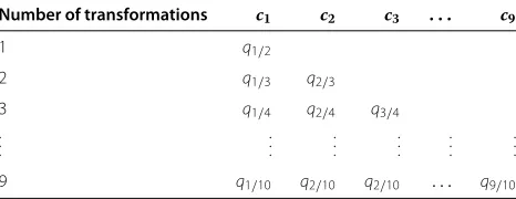
Table 3 Strategy for different categorical transformations: values of the cutpoints for all transformations

Number of transformations c1

k c2k . . . c9k c10k

1 q1/2

2 q1/3 q2/3

. . .

. . .

. . .

. . .

. . .

. . .

9 q1/10 q2/10 . . . q9/10

10 q1/11 q2/11 . . . q9/11 q10/11

Zi (formalized by the correlation ratio(η2)) was specified by the following model:

Zi=β∗Xi(k)+i; (5)

whereXi(k)is the binary coding of theXivariable with a

cutpoint at the median. The coefficientβ∗was computed according toη2and the variance ofXi(k)variable. We tested three different binary codings with cutpoints at the first, the second and the third tercile. The strategy is used for various values of the correlation ratio (η2_{) from 0} to 0.6.

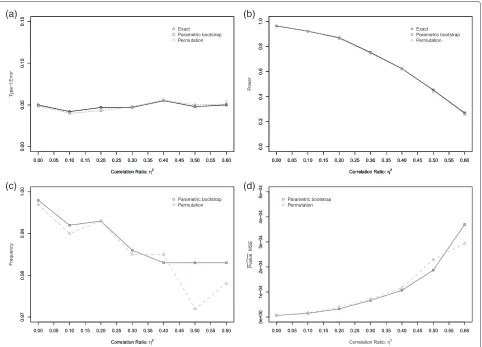
The robustness of the permutation method when the exchangeability assumption is violated was evaluated with respect to the results of the exact method. For differ-ent correlation ratios (η2) we evaluated the control of the Type-I error, the power, the Mean Square Error (MSE) of the estimatedpvalue(pvaluefrom the exact method was

used as a reference), and the rate of good decision (same decision as for the exact method). These results are pre-sented in Figure 4 and show the good behavior of the permutation method since the Type-I error is controlled at the level 0.05, the power is the same for all the meth-ods, the rate of good decision is always greater than 0.97, and the MSE is very low. Moreover, the distributions of the estimatedpvalueare quite similar for different methods

(not shown).

Example: revisiting the PAQUID cohort example

1 2 3 4 5 6 7 8 9 10

0.60

0.70

0.80

0.90

Tests

Po

w

e

r

Bonferroni Parametric bootstrap Permutation

Figure 3Power for an effect of a categorical transformation in five classes defined by cutpoints at the quintile. (γ0= −2.5,γ1=1,βT=(−1.3,−0.8, 1.4, 1.7)).

five Box-Cox transformations for this application, four codings in three classes and four codings in four classes. The best transformation appeared to be the dichotomous transformation of HDL-cholesterol with a cutpoint at the third quartile, as already found by Bonarek et al. [16]. The Bonferroni correction gave apvalueequal to 0.140, thus not

significant for anαlevel at 0.05. Thepvalue, which is given

by both resampling based methods is 0.038. To conclude, it is important to chose a powerful method of correction, because in this context thepvaluewith no correction given

by Bonarek et al. [16] was very optimistic (0.007), and the Bonferroni correction was very conservative, yielding an

(a) (b)

(c) (d)

incorrect conclusion. The proposed approach based on the resampling procedure gave a result which was still significant and more realistic than the uncorrectedp_value.

Discussion

In this paper, we have considered the problem of correc-tion of significance level for a series of several codings of an explanatory variable in a Generalized Linear Model with several adjusting variables. The methods developed, based on resampling methods, enable us to consider categorical transformations as more flexible in order to explore the unknown shape of the effect between an explanatory and a dependent variable. The simulation studies presented above show, firstly, that the resampling method provides similar results for the Type-I error rate control and the power as those found with the exact method proposed by Liquet and Commenges [14] for dichotomous and Box-Cox transformations. Secondly, in the situation of categorical transformations, these simula-tions demonstrate the good performance of our proposed approaches. Finally we observed the robustness estima-tion of thepvalueby the resampling methods. These

meth-ods can be easily generalized to other models, such as the proportional hazards model, and to potentially extend the work of Hashemi and Commenges [15] in the same context.

Conclusion

To conclude, the methods developed, based on resam-pling, demonstrate good performances, and we have implemented different methods and different strategies of coding in an R package called CPMCGLM M (for Correc-tion of the Pvalue after Multiple Coding in a Generalized Linear Model).

Appendix

The package CPMCGLM has been developed in R, an

open source statistical software available at http://www.r-project.org. The methods presented in this paper are avail-able in the main functionCPMCGLM()for Probit, Logit, Linear, and Poisson models. Briefly, the user can spec-ify the transformations tested: Box-Cox, dichotomous or categorical transformations. Two options are possible for defining the cutpoints of the dichotomous and the categorical transformations: the user can either specify them, or the program will automatically use the strat-egy based on the quantile presented in the simulation study.

The main function provides the best codings accord-ing to the maximum test and minimumpvalueprocedures.

For this coding, the different methods of correction of the Type-I error rate presented in this paper are provided. We present an illustration of theCPMCGLMfunction on a simulated dataset:

data(data_sim)

result<-CPMCGLM(formula=

Weight Age+as.factor(Sport)+Desease

+Height,

family="gaussian",link="identity", data=data_sim, varcod="Age",

nb.dicho = 4, nb.categ = 4, nboxcox = 3, N = 10000)

result

Call:

CPMCGLM(formula = Weight Age +

as.factor(Sport) + Desease +

Height, family = "gaussian", link = "identity",

data = data_sim,varcod = "Age", nb.dicho = 4,

nb.categ = 4, nboxcox = 3, N = 10000)

Generalized Linear Model Summary Family: gaussian

Link: identity

Number of subject: 100

Number of adjustment variable: 4

Resampling N: 10000

Best coding

Method: Dichotomous transformation

Value of the order quantile cutpoints: 0.6 Value of the quantile cutpoints: 26.4834

Corresponding adjusted pvalue:

Adjusted pvalue

naive 0.0191

bonferroni 0.2096

bootstrap 0.0686

permutation 0.0656

exact: Correction not available for these codings

Competing interests

Both authors declare that they have no competing interests.

Authors’ contributions

BL and JR developed the methodology, the R code, performed the simulation and the analysis on the dataset as well as wrote the manuscript. Both authors read and approved the final manuscript.

Acknowledgements

Author details

1_{University Bordeaux, ISPED, Centre INSERM}

U-897-Epidemiologie-Biostatistique, Bordeaux, F-33000, France.2_{INSERM, ISPED, Centre INSERM}

U-897-Epidemiologie-Biostatistique, Bordeaux, F-33000, France.3MRC Biostatistics Unit, Institute of Public Health, Cambridge, CB2 0SR, UK.4_Danone

Research, Avenue de la Vauve, Route départementale 128, Palaiseau Cedex 91767, France.

Received: 9 January 2013 Accepted: 17 May 2013 Published: 8 June 2013

References

1. Bennette C, Vickers A:Against Quantiles: categorization of

continuous variables in epidemiologic research, and its discontents.

BMC Med Res Methodol2012,12:21–25.

2. Altman D, Lausen B, Sauerbrei W, Schumacher M:Dangers of using optimal cutpoints in the evaluation of prognostic factors.J Natl Cancer Inst1994,86(11):829–835.

3. Royston P, Altman D, Sauerbrei W:Dichotomizing continuous predictors in multiple regression: a bad idea.Stat Med2006, 25:127–141.

4. Harrell FE, Lee KL, Mark DB:Multivariable prognostic models: issues in developing models, evaluating assumptions and adequacy, and measuring and reducing errors.Stat Med1996,15(4):361–387. 5. Miller RG:Simultaneous statistical inference. 2nd ed. New York - Heidelberg:

Berlin: Springer- Verlag. XVI 299; 1981. figs. DM 44.00.

6. Westfall PH:Improving power by dichotomizing (even under normality).Stat Biopharm Res2011,3(2):353–362.

7. Simes R:An improved bonferroni procedure for multiple tests of significance.Biometrika1986,73(3):751–754.

8. Sidak Z:Rectangular confidence regions for the means of multivariate normal distributions.J Am Stat Assoc1967,62:626–633. 9. Holm S:A simple sequentially rejective multiple test procedure.

Scand J Stat1979,6:65–70.

10. Hommel G:A stagewise rejective multiple test procedure based on a modified Bonferroni test.Biometrika1988,75:383–386.

11. Hochberg Y:A sharper Bonferroni procedure for multiple test procedure.Biometrika1988,75:800–802.

12. Efron B:The length heuristic for simultaneous hypothesis tests.

Biometrika1997,84:143–157.

13. Liquet B, Commenges D:Correction of the P-value after multiple coding of an explanatory variable in logistic regression.Stat Med 2001,20:2815–2826.

14. Liquet B, Commenges D:Computation of the p-value of the minimum of score tests in the generalized linear model, application to multiple coding.Stat Probability Lett2005,71:33–38.

15. Hashemi R, Commenges D:Correction of the p-value after multiple tests in a Cox proportional hazard model.Lifetime Data Anal2002, 8:335–348.

16. Bonarek M, Barberger-Gateau P, Letenneur L, Deschamps V, Iron A, Dubroca B, Dartigues J:between cholesterol, apolipoprotein E polymorphism and dementia: a cross-sectional analysis from the PAQUID study.Neuroepidemiology2000,19:141–48.

17. McCullagh P, Nelder J:Genaralized Linear Models. 2edition. New York: Chapman&Hall; 1989.

18. Genz A:Numerical computation of multivariate normal probabilities.J Comput Graphical Stat1992,1:141–149.

19. Cox D, Hinkley D:Theoretical Statistics. London: Chapman & Hall; 1994. 20. Royen T:Expansions for the multivariate chi-Square distribution.

J Multivariate Anal1991,38:213–232.

21. Dagupsta N, Spurrier J:A class of multivariateχ2_{distributions with}

applications to comparison with a control.Commun Stat- Theory Methods1997,26:1559–1573.

22. Worsley K:An improved Bonferroni inequality and applications.

Biometrika1982,69:297–302.

23. Westfall PH, Young S:Wiley Series in Probability and Mathematical Statistics. Applied Probability and Statistics. New York: NY Wiley; 1992. xvii, 340 p. 24. Yu K, Liang F, Ciampa J, Chatterjee N:Efficientp-value evaluation for

resampling-based tests.Biostatistics2011,12(3):582–593.

25. Commenges D, Liquet B:Asymptotic distribution of score statistics for spatial cluster detection with censored data.Biometrics2008, 64(4):1287–1289.

26. Romano J:On the behavior of randomization tests without a group invariance assumption.J Am Stat Assoc1990,85(411–412):686. 27. Xu H, Hsu J:Applying the generalized partitioning principle to

control the generalized familywise error rate.Biom J2007,49:52–67. 28. Kaizar E, Li Y, Hsu J:Permutation multiple tests of binary features do

not uniformly control error rates.J Am Stat Assoc2011, 106(495):1067–1074.

29. Commenges D:Transformations which preserve exchangeability and application to permutation tests.J Nonparametric Stat2003, 15(2):171–185.

30. Westfall PH, Troendle JF:Multiple testing with minimal assumptions.

Biom J2008,50(5):745–755.

31. Good P:Permutation Tests: Permutation Tests: A Practical Guide to Resampling Methods for Testing Hypotheses. New-York: Springer-Verlag; 2000.

32. Efron B, Tibshirani R:An Introduction to the Bootstrap (Chapman & Hall/CRC Monographs on Statistics & Applied Probability). London: Chapman and Hall/CRC; 1994.

doi:10.1186/1471-2288-13-75

Cite this article as:Liquet and Riou:Correction of the significance level when attempting multiple transformations of an explanatory variable in generalized linear models.BMC Medical Research Methodology201313:75.

Submit your next manuscript to BioMed Central and take full advantage of:

• Convenient online submission

• Thorough peer review

• No space constraints or color figure charges

• Immediate publication on acceptance

• Inclusion in PubMed, CAS, Scopus and Google Scholar

• Research which is freely available for redistribution