Frames, Reproducing Kernels, Regularization and Learning

Frames, Reproducing Kernels, Regularization and Learning

Alain Rakotomamonjy [email protected]

St´ephane Canu [email protected]

Perception, Syst`emes et Information CNRS FRE2645 INSA de Rouen

76801 Saint Etienne du Rouvray, France

Editor: Alex Smola

Abstract

This work deals with a method for building a reproducing kernel Hilbert space (RKHS) from a Hilbert space with frame elements having special properties. Conditions on existence and a method of construction are given. Then, these RKHS are used within the framework of regularization theory for function approximation. Implications on semiparametric estimation are discussed and a multiscale scheme of regularization is also proposed. Results on toy and real-world approximation problems illustrate the effectiveness of such methods.

Keywords: regularization, kernel, frames, wavelets

1. Introduction

A reproducing kernel Hilbert space (RKHS) is a Hilbert space of functions with special prop-erties (Aronszajn, 1950). It plays an important role in approximation and regularization theory as it allows writing in a simple way the solution of a learning from empirical data problem (Wahba, 1990, 2000). Since the development of support vector machines (SVMs) (Vapnik, 1995; Vapnik et al., 1997; Burges, 1998; Vapnik, 1998) as a machine learning for data classification and func-tional estimation, there is a growing interest around reproducing kernel Hilbert spaces. In fact, for nonlinear classification or approximation, SVMs map the input space into a high dimensional feature space by means of a nonlinear transformationΦ (Boser et al., 1992). Usually in SVMs, the mapping function is related to an integral operator kernel K(x,y)which corresponds to the dot product of the mapped data:

K(x,y) =_hΦ(x),Φ(y)_i

where x and y belong to the input space.

In regularization theory (Tikhonov and Ars´enin, 1977; Groetsch, 1993; Morosov, 1984), the ill-conditioned estimation from data problem is transformed into a well-ill-conditioned problem by means of a stabilizer, which is a functional with specific properties.

For both SVMs and regularization theory, one can consider special cases of kernel and stabilizer: the kernel and the norm associated with an RKHS (Girosi, 1998; Smola et al., 1998; Evgeniou et al., 2000). This justifies the appeal of RKHS as it allows the development of a general framework that includes several approximation schemes.

problem since the mapping has a direct influence on the kernel and thus, it has an influence on the solution of the approximation or classification problem. In practical cases, the choice of an appropriate data representation is as important as the choice of the learning machine. In fact, prior information on a specific problem can be used for choosing an efficient input representation, or for choosing a good hypothesis space that leads to enhanced performance of the learning machine (Scholkopf et al., 1998; Jaakkola and Haussler, 1999; Niyogi et al., 1998).

The purpose of this paper is to present a method for constructing an RKHS and its associated kernel by means of frame theory (Duffin and Schaeffer, 1952; Daubechies, 1992). A frame of a Hilbert space spans any vector of the space by linear combination of the frame elements. But unlike a basis, a frame is not necessarily linear independent although it achieves stable representation. Since a frame is a more general way to represent elements of Hilbert space, it allows flexibility in the representation of any vector of the space. By giving conditions for constructing arbitrary RKHS from frame elements, our goal is to widen the choice of kernel so that in future applications, one can adapt its RKHS to prior information available concerning a problem at hand.

The paper is organized as follows: in Section 2, we recall the problem of estimating function from data and the way of solving it owing to regularization theory. Section 3 deals with frame. After a short introduction about frame theory, we give conditions for a Hilbert space described by a frame to be an RKHS and then derive the corresponding kernel. In Section 4, a practical way for building RKHS is given. Section 5 discusses implication of these results on regularization technique and proposes an algorithm for multiscale approximation. Section 6 presents estimation results on numerical experiments on toy and real-world problems while Section 7 concludes the paper and contains remarks and other issues about this work.

2. Regularized Approximation

As argued by Girosi et al. (1995), learning from data can be viewed as a multivariate function approximation from sparse data. Supposing that one has a set of data_{(xi,yi),xi∈Rd,yi ∈R,i=

1. . . `_}provided by the random sampling of a noisy function f , the goal is to recover the unknown function f , from the knowledge of the data set. It is well-known that such a problem is ill-posed as there exists an infinity of functions that pass perfectly through the data. One way to transform this problem into a well-posed one is to assume that the function f presents some smoothness properties and hence, the problem becomes a variational problem of finding the function f∗that minimizes the functional (Tikhonov and Ars´enin, 1977):

H[f] = 1

`

`

∑

i=1

C(yi,f(xi)) +λΩ[f] (1)

whereλis a positive number, C a cost function which determines how differences between f(xi)and yishould be penalized andΩ[f]a functional which denotes the prior information on the function f .

λbalances the trade-off between fitness of f to the data and smoothness of f . This regularization principle leads to different approximation schemes depending on the cost function C(_·,_·). Classical

L2cost function (C(yi),f(xi)) = (yi−f(xi))2leads to the so-called Regularization Networks (Girosi

et al., 1995; Evgeniou et al., 2000) whereas cost function like Vapnik’sε₋insensitive function leads to SVMs.

being related to the inner product bykfk2

H =hf,fiH) , the solution of Equation (1) is under general

conditions

f∗(x) =

`

∑

i=1

ciK(x,xi). (2)

The case of_kf_kH being a seminorm leads to a minimizer with the following form:

f∗(x) =

`

∑

i=1

ciK(x,xi) + m

∑

j=1

djgj(x) (3)

where_{gj}j=1...mspan the null space of the functionalkfk2H.

In a nutshell, looking for a function f of the form (3) is equivalent to minimizing the functional

H[f], and thus the solution which depends onλ is the “best” balance between smoothness in

H

and fitness to the data. Choosing a kernel K is equivalent to specifying a prior information on the RKHS, therefore having a large choice of RKHS should be fruitful for the approximation accuracy, if overfitting is properly controlled, since one can adapt its hypothesis space to each specific data set.

3. Frames and Reproducing Kernel Hilbert Spaces

In this section, we give an introduction to frame theory that will be useful for the remainder of the paper.

3.1 A Brief Review of Frame Theory

Frame theory was introduced by Duffin and Schaeffer (1952) (Daubechies, 1992) in order to establish general conditions under which one can reconstruct perfectly a function f in a Hilbert space

H

from its inner product(_h·,_·iH)with a family of vectors_{φn}n_∈Γ withΓbeing a finite or

infinite countable index set.

Definition 1 A set of vectors_{φn}n∈Γis a frame of a Hilbert space

H

if there exists two constants

A>0 and∞>B_≥A>0 so that

∀f_∈

H

, A_||f_||2_{H ≤}

∑

n∈Γ

|hf,φniH|2≤B||f||2H. (4)

The frame is said to be tight if A and B are equal.

If the set_{φn}n∈Γsatisfies the frame condition then the frame operator U can be defined as

U :

H

−→ `

2

f _{−→ {h}f,φniH}n∈Γ. (5)

The reconstruction of f from its frame coefficients needs the definition of a dual frame. For this purpose, one introduces the adjoint operator U∗of U which exists and is unique because it lies on a Hilbert space:

U∗: `

2 _−→

_H

{cn}n∈Γ −→ ∑n∈Γcnφn.

Theorem 1 (Daubechies, 1992) Let{φn}n∈Γ be a frame of

H

with frame bounds A and B. Let us

define the dual frame_{φ¯n}n_∈Γas ¯φn= (U?U)−1φn. For all f ∈

H

, we have

1

Bkfk

2

H ≤

∑

n∈Γ

|hf,φ¯niH|2≤

1

Akfk

2

H (7)

and

f =

∑

n_∈Γ

hf,φ¯niHφn=

∑

n_∈Γ

hf,φniHφ¯n. (8)

If the frame is tight then ¯φn= 1_Aφn.

This theorem also shows that the dual frame _{φ¯n}n_∈Γ is a family of vectors which allows to

recover any f _∈

H

, and consequently one can write each vector of the frame and the dual frame as

∀m_∈Γ, φ¯m=

∑

n∈Γ

h_φ¯_m,φniHφ¯_{n (9)}

and

∀m_∈Γ, φm=

∑

n_∈Γ

hφm,φniHφ¯n. (10)

According to this theorem and the above equations, one can note that an orthonormal basis of

H

is a special case of frame where A =B=1, ¯φn =φn and kφnk=1. However, as stated

by Daubechies (1992), frame redundancy can be statistically useful. Also note that in the general case, we do not have an analytical expression of the dual frame, and thus it has to be computed numerically. Grochenig has proposed such an algorithm (Grochenig, 1993) which is based on a iterative conjugate gradient method. We have briefly described this algorithm in the appendix but for further details, one should refer to the original paper.

For the sake of simplicity, in the following we will call frameable Hilbert space, a Hilbert space

H

for which there exists a set of vector of

H

that forms a frame of

H

. Note that all separable Hilbert spaces are frameable since by definition they have a countable orthonormal basis.

3.2 A Reproducing Kernel Hilbert Space and Its Frame

After this short introduction on frame theory, let us look at the conditions under which a frame-able Hilbert space is also a reproducing kernel Hilbert space.

First of all, we introduce some notations that will be used throughout the rest of the paper: let

RΩ_{be the set of all functions defined on a domain}Ω_⊂Rd_{with values in}R_.

For the purpose of being self-contained, we propose here some useful definitions and proper-ties concerning RKHS. However, the reader who is interested in deeper details can refer to books describing mathematical aspects (Atteia, 1992; Berlinet and Agnan, 2004).

Definition 2 A Hilbert space

H

with inner product_h·,_·iH is a reproducing kernel Hilbert space of

RΩ_if:

• ∀t∈Ω ,_∃Mt >0 so that

∀f_∈

H

, _|f(t)_{| ≤}Mt||f||. (11)

This latter property means that for any t_∈Ω, the linear functional

F

_t (also called the

evalu-ation functional) defined as

F

t(f):

H

_−→ R

f _−→

F

_t(f) = f(t)

is a bounded linear functional.

Note that for any Hilbert space of functions, the evaluation functional is linear, thus the impor-tant point for having the reproducing kernel property is this evaluational functional being bounded.

Definition 3 We call Hilb(RΩ_{)the set of all RKHS of}RΩ_.

Owing to the Riesz theorem, one can state that:

Theorem 4 Let

H

_∈Hilb(RΩ_{), there exists an unique symmetric function K(·},t)of

H

called the

reproducing kernel of

H

so that

∀t∈Ω, _∀f∈

H

, f(t) =_hf|K(_·,t)_iH. (12)

Theorem 5 Let

H

be a Hilbert space and_{φn}n_∈Γbe a frame of this space. If{φn}n_∈Γis a (finite

or infinite) set of functions ofRΩ_{, so that:}

∀t_∈Ω,

_n

∑

_∈Γ

¯

φn(·)φn(t)

_H

<∞. (13)

Then

H

is a reproducing kernel Hilbert space.

Proof

Step 1 Anyφnis both an element ofRΩand

H

. Hence the equation

∀f_∈

H

, f =

∑

n∈Γ

hf,φ¯niHφn

holds in

H

according to the frame property given in Equation (8) (Mallat, 1998; Daubechies, 1992). Now since,RΩ_{has a structure of vector space, f =}∑_n

∈Γhf,φ¯niφnis also valid inRΩand thus f also

belongs toRΩ_{. Now, if for each t∈}Ω, we define the seminorm on the vector spaceRΩ_as

∀f_∈RΩ_{,kfkt =|f(t)|.}

According to this seminorm, we get the following pointwise convergence:

f=

∑

n∈Γ

hf,φ¯niHφn⇔ f(t) =

∑

n∈Γ

Step 2 Now let’s show that∀t∈Ω, _∃Mt >0 so that

∀f_∈

H

, _|f(t)_{| ≤}MtkfkH. (15)

All elements of

H

can be expanded with regards to the frame elements, so according to Equation (14), we have for all f in

H

andRΩ_:

|f(t)_|=

_n

∑

_∈Γ

hf(_·),φ¯n(·)iHφn(t)

(16) and consequently,

|f(t)_| =

*

f(_·),

∑

n∈Γ ¯

φn(·)φn(t)

+ H

≤ kf_kH

n

∑

_∈Γ

¯

φn(·)φn(t)

_H (17)

by defining Mt,k∑n∈Γφ¯n(·)φn(t)kH one can conclude that

H

is a reproducing kernel Hilbert space

since Mt is finite by hypothesis and therefore,

H

admits an unique reproducing kernel.

Remark 6 In this proof, we have chosen to expand a function f of

H

according to f=∑_n∈Γhf,φ¯niφn.

However choosing the relationship f =∑_n∈Γhf,φniφ¯n would have led to the following equivalent

condition to Equation (13):

∀t_∈Ω,

_n

∑

_∈Γ

¯

φn(t)φn(·)

_H

<∞. (18)

Now let’s try to express the reproducing kernel of such a Hilbert space.

Theorem 7 Let

H

be a reproducing kernel Hilbert space and

H

_∈Hilb(RΩ_{), and the family}

{φn}n∈Γbe a frame of this space, the reproducing kernel is K(s,t)defined by:

K :

Ω_×Ω_→R

s_×t_→K(s,t) =∑n_∈Γφ¯n(s)φn(t) (19)

Proof

At first, note that according to the frame inequality:

∑

n∈Γ φ2

n(t) =

∑

n∈Γ

|hK(t,_·),φn(·)iH|2≤BkK(t,·)k2H <∞.

applying U_φ¯∗ to the `2 sequence{φn(t)} shows that the function∑n∈Γφ¯n(·)φn(t)is a well-defined

function of

H

.

Furthermore, any f _∈

H

can be expanded by means of the frame of

H

, thus according to Equation (14):

f(t) =

∑

n∈Γ

hf,φ¯niHφn(t)

=

*

f(_·),

∑

n∈Γ ¯

φn(·)φn(t)

+

H

(20)

and since

H

is an RKHS, we have

∀f _∈

H

, _∀t_∈Ω, f(t) =_hf(_·),K(_·,t)_iH. (21)

Hence, by identifying Equation (20) and (21) due to the unicity of the reproducing kernel, we have

K(_·,t) =

∑

n∈Γ ¯

φn(·)φn(t)

and thus, we can conclude that

K(s,t) =

∑

n∈Γ ¯

φn(s)φn(t).

These propositions show that a Hilbert space which can be described by its frame is under gen-eral conditions, a reproducing kernel Hilbert space and its reproducing kernel is given by a linear combination of its frame and dual frame product.

A simple corollary to Theorem (7) is that for any RKHS

H

with family_{φn}n∈Γ as a frame, the inequality (13) holds. This naturally stems from the fact that K(_·,t) =∑_n∈Γφ¯n(·)φn(t)is a

well-defined function of

H

(as stated in the proof of Theorem 7) and thus it has a finite norm in

H

. The symmetry and the positivity of the kernel K(s,t) are direct consequences of K(_·,_·) being a kernel of an RKHS. However, these properties can also be easily shown owing to the frame representation. In fact, according to Equation (8) and (14), we get:

x(t) =

∑

n_∈Γ

hx,φ¯niHφn(t) =

∑

n_∈Γ

hx,φniHφ¯n(t)

=

*

x(_·),

∑

n∈Γ ¯

φn(·)φn(t)

+

H

=

*

x(_·),

∑

n∈Γ

φn(·)φ¯n(t)

+

H

(22)

thus, owing to the uniqueness of the functional evaluation in a RKHS, one can deduce from Equation (22) that

K(s,t) =

∑

n∈Γ ¯

φn(s)φn(t) =

∑

n∈Γ ¯

The positivity can also be proved from the following reasoning. Let x1,_···,x`be some vectors ofΩ

and a1,_···,a`some scalar values inR, we want to show that for any set{xi}and{ai}:

`

∑

i,j

aiajK(xi,xj)≥0.

According to Equation (10), we can write

K(xi,xj) =

∑

n∈Γ ¯

φn(xi)

∑

m∈Γ

¯

φm(xj)hφn,φmiH.

Thus, we have

`

∑

i,j

aiajK(xi,xj) =

`

∑

i,j

aiaj

∑

n,m∈Γ ¯

φn(xi)φ¯m(xj)hφn,φmiH

=

* `

∑

i n

∑

_∈Γ

aiφ¯n(xi)φn(·),

`

∑

j m

∑

_∈Γ

ajφ¯m(xj)φm(·)

+

H

=

`

∑

i n

∑

∈Γ

aiφ¯n(xi)φn(·)

2

H ≥ 0.

4. Learning Schemes Using Frames

In the previous section, conditions for a frameable Hilbert space being an RKHS were given. Here, we are interested in constructing a reproducing kernel Hilbert space together with its frame and discuss about the implications of such result in a functional estimation framework.

4.1 Learning on Frameable Hilbert Spaces

An interesting point of frameable Hilbert space is that under weak conditions, it becomes easy to build RKHS. The following theorem proves such point.

Theorem 8 Let N _∈N _{and {}φ_{n}n=1...N be a finite set of non-zero functions of a Hilbert space}

(

B

,_h·,_·i)with

B

_⊂RΩ_{so that}

∃M,_∀t_∈Ω,_∀n 1_≤n_≤N, _|φn(t)| ≤M.

Let

H

be the set of functions so that

H

=_{f=

N

∑

n=1

anφn : an∈R, n=1, . . . ,N}

(

H

,_h·,_·iB)is an RKHS and its reproducing kernel is

K(s,t) =

N

∑

n=1 ¯

φn(s)φn(t),

Proof

Step 1

H

is a Hilbert space.

This is straightforward since

H

is a closed subspace of a Hilbert space

B

, and is endowed with

B

inner product. Hence

H

is a Hilbert space.

Step 2 _{φn}is a frame of

H

. A proof of this step is also given in Christensen (1993). We have

to show that there exists A and B satisfying equation (4). Let us consider the non trivial case that span_{φn}n=1..N6=0.

The existence of B is straightforward applying Cauchy-Schwartz inequality. In fact, for all

f _∈

H

|hf,φni|2≤ kfk2kφnk2

and thus

N

∑

n=1

|hf,φni|2≤ kfk2 N

∑

n=1

kφnk2.

Thus by taking B=∑N_n=1kφnk2, we have B<∞and B satisfies the right-hand inequality of Equation

(4).

Let

H

∗_{,{f ∈}

_H

_{:kfkH >0}and S(f)be the following mapping:}

S :

H

∗ _−→ R

f _−→ S(f) =∑n∈Γ|hf,φni|2. (23)

This mapping is continuous and because

H

∗_{is of finite dimension the restriction of S to the unit} ball in span_{φn}n=1..N reach its infimum (Brezis, 1983): there is g∈span{φn}n=1,...,N withkgk=1

such that

∑

n∈Γ

|hg,φni|2=inf

(

∑

n∈Γ

|hf,φni|2, f ∈

H

∗so thatkfk=1

)

.

Let A be∑n_∈Γ|hg,φni|2. Hence A>0, and askgk=1, one has for any f∈

H

∗:

A_kf_k2_≤

N

∑

n=1

|hf,φni|2.

Step 3 Now let’s prove that

H

is an RKHS. For that it suffices to prove that the frame {φn}

satisfies condition given in Theorem 5.

This is straightforward since_{φn}n=1,...,N is a frame of

H

and owing to Theorem 1, the dual

frame{_φ¯_{n}n=1,...,N is also a frame of}

H

. Hence, the norm of each ¯φn is finite. Besides,|φn(t)|is

supposed to be bounded by M. Hence,

N

∑

n=1 ¯

φn(·)φn(t)

≤M N

∑

n=1

k_φ¯_n(·)k<∞

and consequently,

H

is an RKHS with a kernel equal to:

K(s,t) =

N

∑

n=1 ¯

0 1 2 3 4 5 6 7 8 9 10 −2

−1.5 −1 −0.5 0 0.5 1

x

Amplitude

Frame Elements

Phi1 Phi2

0 1 2 3 4 5 6 7 8 9 10 −14

−12 −10 −8 −6 −4 −2 0 2 4 6

x

Amplitude

Dual Frame Elements

Phi1 Phi2

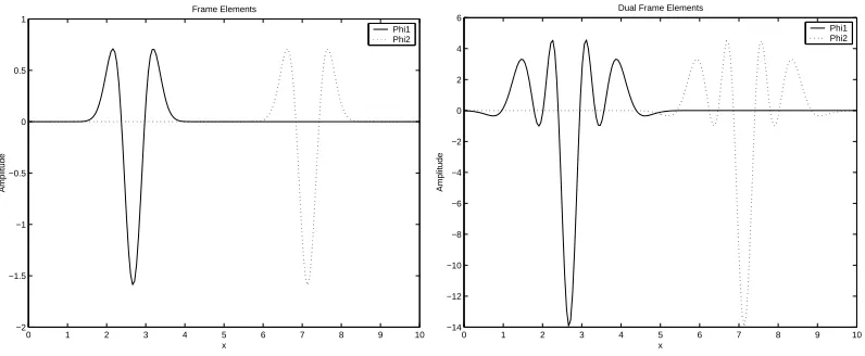
Figure 1: Examples of wavelet frame elements (left) anf their dual elements (right).

Here, we give some examples of RKHS that have been derived from the direct application of this theorem.

Example 1 Any finite set of bounded, real-valued, pointwise-defined and square integrable

func-tions onΩendowed with the inner product_hf,g_i=R

Ωf(t)g(t)dt spans a RKHS. For instance, the

set of functions which expressions are given below spans an RKHS.

∀t_∈Ω,φn(t) =t·e−(t−n)

2

, n_∈[nmin,nmax] with (nmin,nmax)∈N2

Example 2 Any finite set of bounded and pointwise-defined functions belonging to Sobolev space

(Berlinet and Agnan, 2004) spans an RKHS. The set of functions, given in the previous example spans also an RKHS in a Sobolev inner product sense.

Example 3 Consider a finite set of wavelet onR

ψj,k(t) =

1

√

ajψ

t₋ku0aj

aj

,j_∈Z_{: jmin≤ j≤ jmax},k_∈Z_{: kmin≤k≤kmax}

where(a,u0)_∈R∗_+×R_{, and(jmin,jmax,kmin,kmax)∈}Z4_{. Then the span of these functions endowed}

with the inner product_hf,g_i=R

Rf(t)g(t)dt is an RKHS. Figure (1) plots an example of wavelet

frame and dual frame elements for a dilation j=₋7.

The main interest of Theorem (8) is the flexibility it introduces in the RKHS choice or in the choice of the functions that span the hypothesis space. However, this theorem only deals with finite dimension RKHS. For building infinite dimensional RKHS, Theorem (5) has to be used. The main difference between the finite and infinite dimensional case and thus between Theorems (5) and (8) is that a finite set of functions_{φn}n=1,...,N, if endowed with an adequate inner product, is always

Example 4 Let us consider

H

as the space of continuous and differentiable functions onΩ= [0,1]

with the constraints that for any f _∈

H

, f(0) = f(1) =0 and∂f _∈L2(Ω) where ∂f is the usual

derivative of f . Endowed with the inner product:

∀f and g_∈

H

,_hf,g_iH =

Z

Ω∂xf(x)∂xg(x)dx

one can show that

H

is a Hilbert space of functions onΩand that the set

{φn(t)}n∈N∗ =

(√

2

nπ sin(nπt)

)

n∈N∗

is an orthonormal basis of

H

(Debnath and Mikusinki, 1998; Atteia and Gaches, 1999). Hence,

{φn(x)}n∈N∗ is a tight frame of

H

with the frame constant A equals to 1. Let us show that this frame

verify the condition given in Theorem (5) in order to prove that

H

is an RKHS.

At first, let us prove that for all t_∈Ω, the sequence_{φn(t)}n∈N∗ belongs to`₂. Because ¯φ_n=φ_n,

we have for any t_∈Ω:

∑

n∈N∗ φ2

n(t) =

∑

n∈N∗ ¯ φ2

n(t) =

∑

n∈N∗ 2

n2π2sin

2_(nπt)

≤ _π2₂

∑

n_∈N∗ 1

n2 < ∞.

Hence, according to the adjoint frame operator U∗given in equation (6), for any t_∈Ω, the function

∑n∈N∗φn(·)φn(t)is a well-defined function of

H

. Thus,

n

∑

_∈N∗

φn(·)φn(t)

2

H

=

∑

n_∈N∗ φ2

n(t)<∞.

Hence

H

is a infinite dimensional RKHS with kernel

∀s,t_∈Ω,K(s,t) = ∞

∑

n=1 2

n2π2sin(nπs)sin(nπt).

Example 5 This other example shows a way for constructing an infinite dimensional RKHS from

its frame. Let_{αn}n∈Γbe a set of strictly positive real values and define the subspace`2αof`2as

`2_α=

(

c=_{cn}n_∈Γ,cn∈R:

∑

n∈Γ

c2_n

αn

<∞

)

.

Endowed with the inner producthc,di`2

α≡∑n∈Γcαndnn, one can show that`

2

αis a Hilbert space. Now,

let_{φn}n∈Γbe a set of functions onRΩso that:

∀t_∈Ω,

∑

n∈Γ

and T the mapping:

T : `

2

α →

H

⊂RΩ

c _→ f =∑_n∈Γcnφn.

It is simple to show that

H

is a space of functions onΩsince for all t_∈Ω,_{αnφn(t)}n∈Γbelongs to

`2

α. Then we have,

hc,_{αnφn(t)}n∈Γi`2

α=

∑

n∈Γ

cnαnφn(t)

αn

=

∑

n∈Γ

cnφn(t)<∞.

Suppose furthermore for simplicity and clarity that_{φn}n∈Γhas been chosen so that T is an injective

mapping. Then the range of the mapping T also defined as

H

=

(

f =

∑

n∈Γ

cnφn:{cn}n∈Γ∈`2α )

and endowed with the inner product:

hf,g_{iH ≡ h}c,d_i`2

α=

∑

n_∈Γ cndn

αn

with f =

∑

n_∈Γ

cnφnand g=

∑

n_∈Γ dnφn

is also a Hilbert space since in this case T is an isometric isomorphism between`2

αand

H

(Debnath

and Mikusinki, 1998). Note that this way of building a Hilbert space is also described by Opfer (2004a) and Amato et al. (2004). However, none of them has presented the following frame-based

point of view for showing that under some weak hypothesis

H

can be an RKHS.

At first, note that due to the one-to-one mapping between `2

α and

H

, the following equality

holds:

∀k,n_∈Γ, _hφk,φniH =

δk,n

αk

whereδk,nis the Kronecker symbol.

Let us show that_{φn}n∈Γis a frame of

H

. Owing to the above property, we have∑n∈Γ|hf,φni|2=

∑n_∈Γc

2

n

α2

n andkfk

2

H =∑n_∈Γ c

2

n

αn, then it is clear that the following inequality holds:

1 αmaxk

f_k2_{H ≤}

∑

n∈Γ

|hf,φni|2≤

1 αmink

f_k2_H

where αmax =maxn∈Γαn andαmin=minn∈Γαn. Since according to the frame property given in

Equation (8), each frame element can be expanded as φk=∑n∈Γhφk,φniφ¯n, we haveφk = _α1_kφ¯k.

Hence since the frame and dual frame elements are so that for any t_∈Ω, we have

∑

n∈Γ

αnφ2n(t) =

∑

n∈Γ

(φ¯n(t))2

αn

<∞. (24)

Then_{φ¯n(t)}n_∈Γ∈`2_αand consequently, the function K(·,t) =∑n_∈Γφ¯n(t)φn(·)is well-defined,

be-longs by construction to

H

and is so that

_n

∑

_∈Γ

¯

φn(t)φn(·)

_H

and

H

is an RKHS whose kernel is

K(s,t) =

∑

n∈Γ ¯

φn(t)φn(s) =

∑

n∈Γ

αnφn(s)φn(t).

A practical example of such an infinite dimensional RKHS can be obtained as follows. Let us

con-sider thatΩ=R_{and each}φ_{n(t) =} √1

2Jϕ

t−n

2J

with n_∈Z_{, J∈}Z_andϕ(_{t)a pointwise-defined on}Ω

and compactly supported function so that_{φn}n_∈Γare linearly independent. Examples of such

func-tionsϕ(t)are functions that are classically used in wavelet-based multiresolution analysis (Mallat,

1998). Since eachφnis a compactly supported shift of a functionϕ, for any t, the sum in Equation

(24) becomes a finite sum of non-zero terms which convergence is consequently guaranteed for any

{αn}n∈Γ. At this point, we can state that the space

H

=

(

f=

∑

n∈Γ

cn

√

2Jϕ

t₋n

2J

:

∑

n∈Γ

c2_n

αn

<∞

)

is a reproducing kernel Hilbert space.

If we want

H

to be the span of different dilations and shifts ofϕ, we can also show that

H

is

an RKHS by choosing the_{αn}n∈Γto be related to the dilation parameter J so that the inequality in

(24) holds.

4.2 Other Classes of Frame-Based Kernels

Recently, Gao et al. (2001) have proposed another class of frame-based kernels. Their approach is based on the connection between regularization operator and support vector kernel as described in Smola et al. (1998). Supposing that U is the frame operator of a either finite or infinite dimensional RKHS, their kernel is based on the statement that the operator Q=U∗U is a symmetric positive

definite operator and the Green function associated to this operator is a Mercer kernel. Thus, the kernel they proposed, named the frame operator kernel, can be expanded with respect to the dual frame elements as

K(s,t) =

∑

n∈Γ ¯

φn(s)φ¯n(t).

A detailed proof of this equation is given in Gao et al. (2001).

From the point of view of the regularization theory (Smola et al., 1998), this frame-operator kernel of Gao et al. is different from the one we propose as the regularization operator associated to each of them are different. In fact, in our case the regularization operator can be considered as the projector of any function space on

H

whereas in the Gao et al. case, it can be seen as the frame operator U .

More recently, Opfer (2004b) has shown that the kernel associated to an RKHS

H

can be expanded as

K(s,t) =

∑

n∈Γ

φn(s)φn(t)

if and only if the set of functions_{φn}n∈Γ is a super tight frame (which is a tight frame with frame bounds equal to 1) of

H

. This results is a particular case of Theorem (7) since for a super tight frame each dual frame element is ¯φn=φn. Furthermore, compared to Opfer’s work, our Theorem

The works of Amato et al. (2004) and Opfer (2004a) where they both proposed the concept of multiscale kernels can also be related to our work. Interestingly, they have both shown that a Hilbert space spanned by wavelet can be under some weak hypotheses an RKHS. The way they build their RKHS

H

is very similar to the one we described in example (5) and the related reproducing kernel is naturally

K(s,t) =

∑

n∈Γ

αnφn(s)φn(t),

where eachαnis a strictly positive real value. On one hand, Amato et al. ended up with this kernel

by considering that_{φn}n∈Γare a orthonormal wavelet basis of L2([0,1])and showing that for their space

H

, the evaluation functional is continuous. On the other hand, for achieving this result, Opfer has shown that the function K(_·,t) belongs to

H

and satisfies the reproducing property without explicit explanations on how this kernel has been obtained. Hence, although very similar to the work of Opfer, the example (5) gives the functional setting on how the kernel in (Opfer, 2004a) can be derived.

5. Discussions

Propositions presented in previous sections describe a way for easily building RKHS and its associate reproducing kernel. Hence, this kernel can be used within the framework of regularization networks or SVMs for functional estimation.

For SVMs, one usually chooses as a kernel a continuous symmetric function K in L2(Ω)(Ωbeing a compact subset ofRd_{) that has to satisfy the following condition, known as Mercer’s condition:}

Z

Ω

Z

ΩK(x,y)f(x)f(y)dxdy≥0 (25) for all f _∈L2(Ω).

Now, one may ask what are the advantages and drawbacks of using kernels built by means of Theorem (5) or (8).

• Both Mercer’s condition and frameable RKHS allow to obtain a positive definite function. However, it is obvious that conditions for having frameable RKHS are easier to verify than Mercer’s condition. Thus, this can be interpreted as a flexibility for adapting kernel to a particular problem. Examples of this flexibility will be given below within the context of semiparametric estimation. Notice that methods for choosing the appropriate frame elements of the RKHS are not given here.

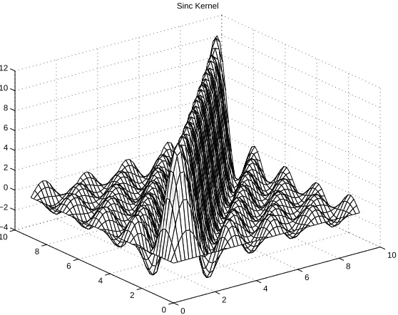
Example 6 Consider the set of functions onR n

φn(s) =sin_π((π(_s−s−_n)n))

o

n=1...N. The space spanned

by these frame elements associated to L2(R_{) inner product is an RKHS. Thus, as a direct}

corollary of Theorem 8, the kernel

K(s,t) =

N

∑

i=1 ¯

φi(s)φi(t)

is an admissible kernel for SVMs.

0 2

4 6

8 10

0 2 4 6 8 10 −4 −2 0 2 4 6 8 10 12

Sinc Kernel

Figure 2: The sinc kernel.

• Since conditions for obtaining a frameable RKHS hold mainly for finite dimensional space (although, it may exists infinite dimensional Hilbert space which frame elements satisfy hy-potheses of Theorem (5)), it is fairest to compare the frameable kernel to a finite dimensional kernel. According to Mercer’s condition, or other more detailed papers on the subject (Aron-szajn, 1950; Wahba, 2000), Mercer’s kernel can be expanded as follows:

K(s,t) =

N

∑

n=1 1 λn

ψn(s)ψn(t)

where s and t belong toΩ,λl is a positive real number and{ψl}i=1..N is a set of orthogonal

functions. Conditions for constructing frameable kernel are less restricting since the orthogo-nality of the frame elements are not needed. One can note that for tight frame or orthonormal basis, frameable kernel leads to the following expansion:

K(s,t) =

N

∑

n=1 1

Aψn(s)ψn(t)

since dual frame elements is equal to frame elements up to a multiplicative constant depending on the frame bound A . Tightness of a frame is a very interesting property since in this case processing the dual frame is no more needed. However, unless we explicitly build the RKHS

• The conditions for a frameable Hilbert space being an RKHS is given in Equation (13) and they hold also for infinite dimensional case for which the kernel is written

K(s,t) =

∑

n

¯

φn(s)φn(t).

Again in this case, the frame kernel expansion is similar to the Mercer’s kernel one. The main difference between the finite and infinite dimensional case relies on the fact that a finite set of functions_{φn}is always a frame of the space it spans (provided that this latter is endowed

with an adequate inner product). This is not always true for an infinite set of functions. However, we have shown in example (5) that under some mild conditions, it is possible to build an infinite dimensional RKHS.

• In the SVMs algorithm, the kernel realizes the dot product of the data points mapped in some feature space:

K(s,t) =_hΦ(s),Φ(t)_i

withΦbeing the mapping. Usually, this mapping is not explicitly given since one only needs for computing the optimal hyperplane the dot product in the feature space. With frame-based kernels, we have the relation

K(s,t) =

N

∑

n=1 ¯

φn(s)φn(t)

=

N

∑

n=1 ¯ φn(s)

N

∑

j=1 ¯

φj(t)hφj(·),φn(·)iH according to Equation (10)

=

*

N

∑

n=1 ¯

φn(s)φn(·), N

∑

j=1 ¯

φj(t)φj(·)

+

H

.

Thus the data embedding can be defined as

Φ: Ω −→

H

t _−→ ∑N_n=1φ¯n(t)φn(·).

The data points are mapped to a function belonging to

H

. The mapping is consequently strictly related to the frame elements_{φn}and is implicitly defined by them.

• Besides, since the kernel has an expansion with regards to the frame elements, the solution of Equation (1) is of easier interpretation. Indeed, although the solution depends on the kernel expression, it can be rewritten as a linear combination of the frame elements. Thus, compared to other kernels for which basis functions are unknown, using frame-based kernel increases model interpretability.

to process the kernel matrix K with elements Ki,j=K(xi,xj). Thus, with frame-based kernel,

one has to compute the dual frame elements, (for instance, by means of an iterative algorithm, as the one described in (Grochenig, 1993)). This by its own may be time-consuming. Further-more, the construction of the matrix K needs the processing of the sum. Hence, if the number

N of frame elements describing the kernel and the number `of data are large, building K

becomes rapidly very time-consuming (of an order of N2_·`2).

Some of these points suggest that frame-based kernels can be useful by themselves. However, within the context of semiparametric estimation, this flexibility for building kernel offers some other interesting perspectives. Semiparametric estimation can be introduced by the following theorem.

Theorem 9 (Kimeldorf and Wahba, 1971)

Let

H

Kbe an RKHS of real valued functions onΩwith reproducing kernel K. Denote by{(xi,yi)i=1...`}

the training set and let_{gj,j=1. . .N}be a set of functions onΩsuch that the matrix Gi,j=gj(xi)

has maximal rank. Then, the solution to the problem

min

f∈span(g)+h,h∈HK

1 `

`

∑

i=1

C(yi,f(xi)) +λkfk2HK (26)

has a representation of the form

f(_·) =

`

∑

i=1

ciK(xi,·) + N

∑

j=1

djgj(·).

The solution of this problem can be interpreted as a semiparametric estimation since one part of the solution (the first sum) comes from a non-parametric estimation (the regularization problem) while the other term is due to the parametric expansion (the span of _{gj}). As stated by Smola in his

thesis (Smola, 1998), semiparametric estimation can be advantageous with regards to a fully non parametric estimation as it exploits some prior knowledge on the estimation problem (for instance major properties of the data are described by linear combination of a small set of functions), and making a “good” guess (on the set of functions_{gj}) can have a large effect on performance.

Again in this context, the flexibility of frame-based kernel can be exploited. In fact, let G=

{gi}i=1...N be a set of N linearly independent functions that satisfies Theorem 8, hence, any subset

of G,_{gi}i∈Γ,(Γbeing an index set of size n0<N) can be used for building an RKHS

H

K while

the remaining vectors can be used in the parametric part of the Kimeldorf-Wahba theorem. Hence in this case, the solution of (26) is written

f(_·) =

`

∑

i=1

ci

∑

k∈Γ ¯

gk(xi)gk(·) +

∑

j_∈CΓ

djgj(·).

H

0

@ @

@ R

F

0

H

₁

@ @

@ R

F

1

H

₂

@ @

@ R

F

₂

H

₃

Figure 3: Example of multiscale approximation on 3 levels. Each space

H

j can be decomposed in

a trend space

H

_j−1and a detail space

F

_j−1. In this case,

H

₃can be considered as the sum of

H

0,

F

0,

F

₁and

F

2.

. ∑djΦj(x)

?

∑cjKj(x,xi)

@ @

@ @

@_@R

noise ∑dj,1Φj,1(x)

?

∑cj,1Kj,1(x,xi)

@ @

@ @

@@R

noise ∑dj,2Φj,2(x)

?

∑cj,2Kj,2(x,xi)

@ @

@ @

@@R

noise (xi,yi)i=1,n

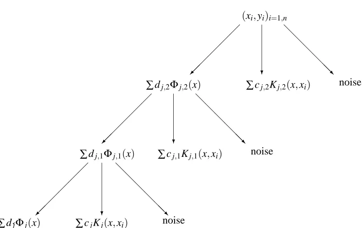
Figure 4: Example of multiscale approximation on 3 levels: the kernel point of view. For instance, here we want to learn a function f(x) that has generated the samples(xi,yi)i=1,n under

some noisy condition. The first step consists of decomposing the hypothesis space into a parametric part spanned by_{Φj,2(x)}and a non parametric part spanned by Kj,2(x,xi).

Then the resulting parametric approximation is decomposed again in two parts and so on. The multiscale approximation of f(x) is then ˆf(x) =∑djΦj(x) +∑cjKj(x,xi) +

the subset of G which is used in the parametric part has to be linearly independent.

Another perspective which follows directly from this finding is a technique of regularization that we call multiscale regularization which is inspired from the multiresolution analysis of Mallat (1998). Here, we just sketch the idea behind this concept and in no way, the following paragraph should be considered a complete study of this new technique since the analysis of its properties goes beyond the scope of this paper. Consider the same problem as the one described in Theorem 9. Now, suppose that_{gi}is a set of N linearly independent functions verifying Theorem (8). Let

{Γi}i=0...mbe a set of index set such that∪mi=0Γi={1, . . . ,N}andΓi∩Γj=/0for i6=j and

H

being

the RKHS spanned by _{gi}. By subdividing the set {gi} with the index set{Γi}i=0...m, one can

construct m RKHS_{

F

_{i}i=0...m−1}in such a way that

∀i=1. . .m,

F

_i−1=span_{gk}k∈Γi

and reproducing kernel of

F

_iis noted Ki. Now, denote as

H

ithe RKHS such that

∀i=1. . .m,

H

_i=

H

_i−1+

F

_i−1

with

H

₀=span_{gk}k∈Γ0. By construction, the space

H

iare nested spaces:

H

0⊂

H

1⊂. . .⊂

H

m=

H

.

In this case, one can interpret

H

₀as the space of lower approximation capacity whereas

H

_mis the space with higher capacity. Besides, since

H

_i=

H

_i−1+

F

_i−1, one can think of

F

_i−1as the details needed to be added to

H

_i−1 to obtain

H

_i, thus we will call spaces

F

_i the “details” spaces whereas spaces

H

_i are the “trend” spaces. Every of these spaces

F

_iand

H

_i are an RKHS since any subset of

{gi}satisfies Theorem (8).

Multiscale regularization is an iterative technique that at step k=1, . . . ,m consists of looking

for the solution fm−k(·)of the following minimization problem:

min

f∈Hm−k+1

1

n n

∑

i=1

C(yi,m−k,f(xi)) +λm−kkfk2Fm−k (27)

where yi,m₋1=yi, yi,m−(k+1)=yi,m₋k−∑nj=1cj,m₋kKm₋k(xj,xi). According to the representer

The-orem (9), fm−k(·)can be written:

fm−k(·) = n

∑

i=1

ci,m−kKm−k(xi,·) +

∑

j_∈∪m−k

l=0Γl

dj,m−kgj(·) (28)

and thus the overall solution of the so-called multiscale regularization is

ˆ

f(_·) =

m

∑

k=1

n

∑

i=1

ci,m₋kKm₋k(xi,·) +

∑

j∈Γ0

dj,0gj(·). (29)

The solution ˆf of the multiscale regularization is the sum of different approximations on nested

so on. Thus at each step, one can control the “amount” of regularization brought to each details space, increasing in this way the capacity control capability of the model. Figure (3) and (4) show an example of how the algorithm works for a 3-level approximation scheme.

The framework of additive models of Hastie et al. (Hastie and Tibshirani (1990)) can give other insights to multiscale regularization. In fact, if we suppose that the family _{gi}i=1,...,N forms an

orthonormal basis of

H

and build the spaces

H

₀and

F

_min the same way as described above, then by construction, we have

H

=

H

0⊕

F

0⊕ ··· ⊕

F

m₋1.

Hence any function f _∈

H

can be written as f(x) =∑m_i=0fi(x) with f0 ∈

H

0 and fi ∈

F

i₋1 for

i=1, . . . ,m. Thus, the multiscale regularization algorithm can be interpreted as an algorithm which

looks for the function f that minimizes the following empirical risk:

Rreg[f] =

1 `

`

∑

i=1

C(yi, m

∑

j=0

fj(xi)) + m

∑

j=1

λjkfjk2Fj−1 (30)

where eachλj is a hyperparameter that controls the amount of regularization for

F

j₋1. This

min-imization problem is typically the problem of fitting an additive model as proposed by Hastie and Tibshirani (1990).

Illustrations of the multiscale regularization algorithm on both toy and real-world problems are given in the next section.

6. Numerical Experiments

This section describes some experiments that compare frame-based kernels to classical one (for instance gaussian kernel) on some regression problems. Besides, illustrations of some points raised in the discussion such as the multiscale approximation algorithm are given.

6.1 Experiment 1

This first experiment aims at comparing the behavior of different kernels using regularization networks and support vector regression. The function to be approximated is

f(x) =sin x+sinc(π(x₋5)) +sinc(5π(x₋2)) (31)

where sinc(x) =sin x_x . Data used for the approximation is corrupted by an additive noise, thus yi= f(xi)+εiwhereεiis a zero-mean gaussian noise of standard deviation 0.2 . Points xiare drawn from

uniform random sampling of interval[0,10]. Three kernels have been used for the approximation:

• Gaussian kernel:

K(x,y) =e−k

x−yk2

2σ2

• Wavelet kernel:

K(x,y) =

∑

i∈Γ ¯

ψi(x)ψi(y)

where i denote a multi index and ψi(x) =ψj,k(x) = √1_ajψ

x−ku0aj

aj

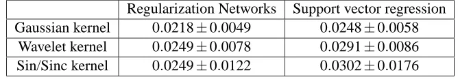
Regularization Networks Support vector regression Gaussian kernel 0.0218_±0.0049 0.0248_±0.0058

Wavelet kernel 0.0249_±0.0078 0.0291_±0.0086 Sin/Sinc kernel 0.0249_±0.0122 0.0302_±0.0176

Table 1: True generalization error for Gaussian, Wavelet, Sin/Sinc kernels with Regularization Net-works and support vector regression for the best hyperparameters.

in the set_{−5,0,5_}whereas k is chosen so that a given waveletψj,k(x)has its support in the

interval[0,10]. For now on, we set u0=1 and a=20.25. These values are those proposed by Daubechies (Daubechies, 1992) so that a wavelet set is a frame of L2(R). Notice that in our case, we only use a subset of this frame.

• Sin/Sinc kernel:

K(x,y) =

∑

i_∈Γ

¯

φi(x)φi(y)

whereφi(x) ={1,sin(x),cos(x),sinc(jπ(x−k)): j∈ {1,3,6},k∈[1. . .9])}.

For frame-based kernel, if necessary the dual frame is processed using Grochenig’s algorithm. For both regularization network and support vector regression, some hyperparameters have to be tuned. Different approaches are possible for solving this model selection problem. In this study, the true generalization error has been evaluated for a range of finely sampled values of hyperpa-rameters. This is repeated for a hundred different data sets, and the mean and standard deviation of the generalization error are thus obtained. Table 1 depicts the true generalization error evaluated on 200 datapoints for the two learning machines and the different kernels using the best hyperpa-rameters setting. Analysis of this table leads to the following observation: The different kernels and learning machines give comparable results (all averages are within one standard deviation from each other). Using prior knowledge on the problem in this context does not improve performance (Sin/Sinc kernel or wavelet kernel compared to gaussian kernel). A justification can be that such kernels use strong prior knowledge (the sin frame element) that is included in the kernel expansion and thus this prior knowledge gets regularized as much as other frame elements. This suggests that semiparametric regularization should be more appropriate to get advantage of such a kernel.

6.2 Experiment 2

In this experiment, we suppose that some additional knowledge on the approximation problem is available, and thus its exploitation using semiparametric approximation should lead to better performance. We have kept the same experimental setup as the one used in the first example but we have restricted our study to regularization networks.

Basis functions and kernel used are the following:

• Gaussian kernel and sinusoidal basis functions_{1,sin(x),cos(x)_}.

• Gaussian kernel and wavelet basis functions

n

ψj,k(x) =√1_ajψ

x−ku0aj

aj

,j_{∈ {}0,5_}

• Wavelet kernel and wavelet basis functions: these functions are the same as in the previous case but the kernel is built only with low dilation wavelet ( j=₋10). In a nutshell, we can consider that the RKHS associated to the kernel used in the non- parametric context (experiment 1) has been splitted in two RKHS. One that leads to a hypothesis space that have to be regularized and another one that does not have to be controlled.

• Sinc kernel and Sin/Sinc basis functions: in this setting, the kernel is given by the following equation:

K(x,y) =

∑

i∈Γ ¯

φi(x)φi(y)

withφi(x) ={sinc(jπ(x−k)): j∈ {3,6},k∈[1. . .9]}

and the basis functions are_{1,sin x,cos x,sinc(π(x₋k): k_∈[1. . .9]_}.

For each kernel, model selection has been solved by cross-validation using 50 data sets. Then, after having spotted the best hyperparameters, the experiment was run a hundred times and the true generalization error in a mean-square sense, was evaluated. Table 2 summarizes all these trials and describes the performance improvement achieved by different kernels compared to the gaussian kernel and sin basis functions. From this table, one can note that:

- exploiting prior knowledge on the function to be approximated leads immediately to a lower generalization error (compare Table 1 and Table 2).

- as one may have expected, using strong prior knowledge on the hypothesis space and the related kernel gives considerably higher performances than gaussian kernel. In fact, the sinc-based kernel achieves by far the lower mean square error. The idea of including the “good” knowledge in a non-regularized hypothesis space while including the “bad” prior knowledge in the RKHS span seems to be fruitful in this case (the frame elements sinc(3π(x₋k))and sinc(6π(x−k))can be termed as “bad” knowledge as, they are not used in the target function ).

- wavelet kernel achieves minor improvement of performance compared to gaussian kernel. However, this is still of interest as using wavelet kernel and basis functions does corresponds to prior knowledge that can be reformulated as: “the function to be approximated contains smooth structure (the sin part), irregular structures (the sinc part) and noise”. It is obvious that knowing the true basis function leads to better performance, however that information is not always available and using bad knowledge may result in poorer performance. Thus, prior knowledge on structures which may be easiest to get than prior knowledge on basis function can be easily exploited by means of wavelet span and wavelet kernel.

6.3 Experiment 3

Kernel / Basis Functions M.S.E Improvement (%) Gaussian / Sin 0.0216_±0.0083 (6) 0

Gaussian / Wavelet 0.0202_±0.0072 (4) 4.6 Wavelet / Wavelet 0.0195_±0.0077 (2) 9.7 Sinc / Sin 0.0156_±0.0076 (88) 27.8

Table 2: True generalization performance for semiparametric regression networks and different set-tings of kernel and basis functions. The number in parentheses reflects the number of trials for which the model has been the best model.

0 1 2 3 4 5 6 7 8 9 10 −2

−1 0 1 2 3 4 5 6 7 8

x

Amplitude

(a)

0 1 2 3 4 5 6 7 8 9 10 −2

−1 0 1 2 3 4 5 6 7 8

x

Amplitude

(b)

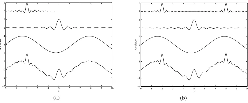
Figure 5: Original functions used for benchmarking in experiment 3. (a) f1(b) f2. Top: multiscale structure on 3 levels. Bottom: Complete function.

and basis functions are taken. The true functions used for benchmarking are the following:

f1(x) = sin x+sinc(3π(x₋5)) +sinc(6π(x₋2)),

f2(x) = sin x+sinc(3π(x−5)) +sinc(6π(x−2)) +sinc(6π(x−8)).

The two functions f1and f2have been randomly sampled on the interval[0,10]. Gaussian noiseεi

of standard deviation 0.2 is added to the samples, thus the entries of the learning machines become

{xi,f(xi) +εi}. Here again, a range of finely sampled values of hyperparameters has been tested

for model selection. In each case, an averaging of the true error generalization over 100 data sets of 200 samples was evaluated using a uniform measure.

For semiparametric regularization, the kernel and basis setting was built with a wavelet set given by

ψj,k(x) =

1

√

ajψ

x₋ku0aj

aj

f1 f2 Gaussian Reg. Networks 0.0266_±0.0085 0.0385_±0.0141

Gaussian SVM 0.0328_±0.0093 0.0475_±0.0155 Semip Reg. Networks 1 0.0266_±0.0085 0.0397_±0.0113 Semip Reg. Networks 2 0.0236_±0.0063 0.0353_±0.0080 Multi. Regularization 0.0246±0.0060 0.0344±0.0069

Table 3: True mean-square-error generalization for regularization networks, SVM, semiparametric regularization networks, and multiscale regularization for f1and f2.

The kernel is constructed from a set of wavelet frame of dilation jSPH and the basis functions

are given by another wavelet set described by jSPL. For multiscale regularization, the setting of the

nested spaces are the following:

H

₀=span

1

√

ajψ

t₋ku0aj

aj

,j=5

,

F

₀=span

1

√

ajψ

t₋ku0aj

aj

,j=0

,

F

₁=span

1

√

ajψ

t₋ku0aj

aj

,j=₋10

.

These dilation parameters have been set in a ad hoc way, but their choices can be justified by the following reasoning: Three distinct levels have been used for separating the approximation in three structures which should be smooth ( j=5), irregular ( j=0) and highly irregular ( j=₋10). The same values of j were used in the semiparametric context. Two semiparametric settings have been tested: the first one uses jSPH =−10 and jSPL={0,5}and the other one is configured as follows

jSPH={−10,0}and jSPL=5.

Table 3 presents the average of the mean-square error of the different learning machines for the two functions and for the best hyperparameter value found by cross-validation. Comments and analysis of this experiment validating the concept of multiscale approximation are:

- semiparametric 2 and multiscale approximation give the best mean-square error. They achieve respectively a performance improvement with regards to gaussian regularization networks of 11.2% and 7.5% for f1, and 8.3% and 10.6% for f2. Also note that both learning machines give the lowest standard deviation of the mean square error.

- multiscale approximation balances loss of approximation due to error at each level (see Fig-ure) and flexibility of regularization, thus its performance is better than semiparametric one’s when the multiscale structure of the signal is more pronounced.

0 1 2 3 4 5 6 7 8 9 10 −2

−1 0 1 2 3 4 5 6 7 8

Amplitude

Multiscale Approximation

x

0 1 2 3 4 5 6 7 8 9 10 −2

−1 0 1 2 3 4 5 6 7 8

x

Amplitude

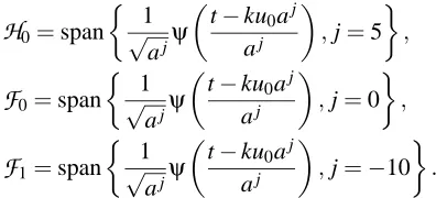
Figure 6: Top: Multiscale structure of a typical prediction of of f1(left) and f2(right) by multiscale wavelet approximation Bottom: full approximation and true function

0 1 2 3 4 5 6 7 8 9 10 −1.5

−1 −0.5 0 0.5 1 1.5 2

x Example of approximation

Amplitude

Original SemiParam2 MultiReg Regnet

0 1 2 3 4 5 6 7 8 9 10 −1.5

−1 −0.5 0 0.5 1 1.5 2

x

Amplitude

Example of approximation Original SemiParam2 MultiReg Regnet