A Robust Procedure For Gaussian Graphical Model Search From
Microarray Data With p Larger Than n
Robert Castelo [email protected]
Departament de Ci`encies Experimentals i de la Salut Universitat Pompeu Fabra
Dr. Aiguader 88, E-08003 Barcelona, Spain
Alberto Roverato [email protected]
Dipartimento di Scienze Statistiche Universit`a di Bologna
Via Belle Arti 41, I-40126 Bologna, Italy
Editor: Max Chickering
Abstract
Learning of large-scale networks of interactions from microarray data is an important and challeng-ing problem in bioinformatics. A widely used approach is to assume that the available data consti-tute a random sample from a multivariate distribution belonging to a Gaussian graphical model. As a consequence, the prime objects of inference are full-order partial correlations which are partial correlations between two variables given the remaining ones. In the context of microarray data the number of variables exceed the sample size and this precludes the application of traditional structure learning procedures because a sampling version of full-order partial correlations does not exist. In this paper we consider limited-order partial correlations, these are partial correlations computed on marginal distributions of manageable size, and provide a set of rules that allow one to assess the usefulness of these quantities to derive the independence structure of the underlying Gaussian graphical model. Furthermore, we introduce a novel structure learning procedure based on a quantity, obtained from limited-order partial correlations, that we call the non-rejection rate. The applicability and usefulness of the procedure are demonstrated by both simulated and real data. Keywords: Gaussian distribution, gene network, graphical model, microarray data, non-rejection rate, partial correlation, small-sample inference
1. Introduction
the so-called microarray data, can be seen as a random sample of a multivariate distribution de-fined by a set of random variables associated to the genome functional elements under study (e.g., genes). Each record corresponds to a vector of values describing the abundance of a particular kind of biomolecule (e.g., messenger RNA) produced by each genome functional element under a specific experimental condition (e.g., a specific tissue or cell line). Thus, a way to describe the interactions among the genome functional elements is by using conditional independencies and, more concretely, graphical models (see Pearl, 1988; Whittaker, 1990; Lauritzen, 1996) which have emerged as a powerful tool for the learning, description and manipulation of conditional indepen-dencies.
However, in a typical microarray data set the number of observations n (on the order of tens) is substantially smaller than the number of variables p (on the order of hundreds or even thousands) and this prevents us from applying directly most of the existing multivariate methods for structure learning of graphical models due to the difficulties in obtaining estimates of the joint probability distribution.
In this paper, we focus in Gaussian graphical models and investigate the role of marginal dis-tributions in their structure learning. Firstly, we formally introduce the concept of q-partial graph that is a graph associated with the set of all marginal distributions of dimension q+2 and, fur-thermore, we provide a comprehensive description of the connection between a q-partial graph and the graph associated with the Gaussian graphical model of interest. Secondly, we propose a novel
q-partial-correlations based procedure, qp-procedure hereafter, for structure learning of q-partial
graphs based on a quantity that we call the non-rejection rate. The results of this paper can be applied also outside the biological context because they can be more generally useful whenever structure learning of a Gaussian graphical model is carried out in the special context in which (i) p is large compared to n, (ii) the underlying structure of the graphical model is sparse. Furthermore, the qp-procedure can also be regarded as a method to obtain shrinkage estimators of the covariance matrix. We remark that the theory of q-partial graphs is developed under the assumption of
faithful-ness of the probability distribution to its independence graph, however the qp-procedure is robust
with respect to this assumption as we shall discuss at the end of the paper.
The paper is organized as follows. Sections 2 and 3 give the theory of Gaussian graphical models and their application to learning of biomolecular networks from microarray data, respectively. The theory of q-partial graphs is given in Section 4 whereas the required graph theory is provided in the Appendix. The qp-procedure is introduced in Section 5 where instances of its application to both simulated and real data are given and, finally, Section 6 contains a brief discussion.
2. Gaussian Graphical Models
In this section we review the Gaussian graphical model theory required for this paper. For a full account of graphical model theory we refer to Cox and Wermuth (1996), Lauritzen (1996) and Whittaker (1990) whereas, for the theory relating to structure learning of graphical models we refer to Cowell et al. (1999), Edwards (2000), Jones et al. (2005) and Whittaker (1990).
Let XV ≡X be a random vector indexed by V ={1, . . . ,p}with probability distribution PV and let G= (V,E)be an undirected graph; see Appendix A for the graph theory used here. For a subset
A⊆V , we denote by XAthe subvector of X indexed by A, and by PAthe associated marginal
We say that PV is (undirected) Markov with respect to G if it holds that XI⊥⊥XJ|XU whenever U sep-arates I and J in G; in particular this implies that if(i,j)∈E then X¯ i⊥⊥Xj|XV\{i,j}. Here ¯E denotes the set of missing edges of G= (V,E)as formally defined in Appendix A. We say that PV is faithful to G if all the conditional independence relationships in PV can be read off the graph G through the Markov property. Consider a graph G0= (V,E0)larger than G, G⊆G0. It is straightforward to check that if PV is Markov with respect to G then it is also Markov with respect to G0. However, if
PV is faithful to G then it is faithful to G0 if and only if G=G0.
Throughout this paper XV is assumed to have a multivariate normal distribution with mean
vector µV and positive definite covariance matrixΣVV≡Σ. Furthermore, we assume that PV is both Markov and faithful with respect to an undirected graph G= (V,E). Hence, for a subset Q⊂V with i,j6∈Q it holds that Xi⊥⊥Xj|XQif and only if the partial correlation coefficient
ρi j.Q=
−κA
i j q
κA iiκAj j
is equal to zero, where A=Q∪ {i,j} and KA ={κA
i j} is the concentration matrix of XA, KA=
(ΣAA)−1(Lauritzen, 1996, p. 130). Of special interest is the case A=V because the concentration matrix KV ≡K={κi j}is the inverse ofΣand the structure of G= (V,E)can be derived from the zero pattern of K. More specifically, it holds that (Lauritzen, 1996, Proposition 5.2)
ki j=0 ⇔ ρi j.V\{i,j}=0 ⇔ (i,j)∈E¯, (1)
and for this reason G is called the concentration graph of XV. For|Q|=q, the parameterρi j.Qis called a q-order partial correlation of Xiand Xj, and if q=p−2, that is, Q=V\{i,j}, we say that
ρi j.Qis the full-order partial correlation of Xiand Xj.
A Gaussian graphical model (Dempster, 1972) is the family of p-variate normal distributions that are Markov with respect to a given undirected graph G= (V,E). Let X(n)= (X1, . . . ,Xn)be a random sample from PV. For a Gaussian graphical model with graph G the sufficient statistics are given by the sample mean vector and by the sample covariance matrices SCCfor C∈
C
whereC
is the set of cliques of G (Lauritzen, 1996, p. 132). It follows that, when G is complete the sufficient statistics are the sample mean and the sample covariance matrix S. Here, we consider problems in which the sample size is small, and it is thus important to recall that, for A⊆V , the samplecovariance matrix SAAfrom XA(n)has full rank, with probability one, if and only if n>|A|(Dykstra, 1970) and that a necessary condition for the computation of several statistical quantities such as the maximum likelihood estimates of K and of the partial correlations in (1) is that SCChas full rank for all C∈
C
.Structure learning aims at identifying the structure G= (V,E)with the fewest number of edges on the basis of the available data such that the underlying distribution PV is undirected Markov over
G. In a frequentist approach to inference, a basic operation to be performed in structure learning
procedures is a statistical test for the hypothesis that a given partial correlation is zero,ρi j.Q=0, since for Q=V\{i,j}this is equivalent to the hypothesis that(i,j)∈E. If, for A¯ =Q∪ {i,j}, XA has an (unrestricted) normal distribution then the generalized likelihood ratio test for the hypothesis
thatρi j.Q=0 has form L=−n log(1−ρˆi j2.Q) where ˆρi j.Q=−κˆAi j/ q
ˆ κA
statistical test may be preferred; see Sch¨afer and Strimmer (2005a). An alternative way to verify the above hypothesis is provided by the connection between partial correlations and regression coefficients. More specifically, in the regression of Xion XA\{i}the regression coefficient associated
with Xjis zero if and only ifρi j.Q=0 (see Cox and Wermuth, 1996, p. 69). In the structure learning procedure proposed in this paper, to verify the absence of an edge from the unrestricted model we will apply the usual t test for zero regression coefficients because it is optimal, in the sense that it is Uniformly Most Powerful Unbiased (UMPU) (see Lehmann, 1986, p. 397).
3. Gaussian Graphical Models For biomolecular Networks
Microarray data quantify the abundance of biomolecules, commonly known as expression level, by probing functional elements along the genome which, without loss of generality, we shall hereafter refer to as genes. A set of p genes being probed define a vector of random variables Xi, i=1, . . . ,p, that take normalized values of the expression levels of the corresponding genes. For every variable
Xithere is vector of n values coming from n different experimental conditions forming the so-called expression profile. The microarray data consist of the expression profiles of a set of genes and form a snapshot of the interactions between the genes in terms of statistical (in)dependencies which, in principle, could be inferred through structure learning of Gaussian graphical models and thus leading to a description of the underlying biomolecular network in these terms. Hence, the prime object of interest is the inverse of the covariance matrix, also known as concentration matrix, whose zero pattern defines the structure of the graphical model, known then as concentration graph.
However, in contrast with the usual data sets found in the literature, on which structure learning of Gaussian graphical models is applied, microarray data constitute a challenging problem because microarray experiments typically measure the expression level of a large number of genes across a small number of experimental conditions. As a consequence of the scarcity of the data, the max-imum likelihood of the inverse covariance matrix does not exist because the sample covariance matrix has full rank, with probability one, if and only if n>p (Dykstra, 1970). This paper tackles
this specific circumstance under which we perform structure learning of Gaussian graphical models with small n and large p.
An important observation in this context is that a growing body of biological evidence suggests that biomolecular networks have a sparse structure. This feature, usually regarded as an advantage, has been exploited in a number of ways to enable learning of Gaussian graphical models from microarray data (see, among others, Wong et al., 2003; Dobra et al., 2004; Wille et al., 2004; Wille and B¨uhlmann, 2006; Sh¨afer and Strimmer, 2005a, 2005b, 2005c) among which some methods work by obtaining shrinkage estimators of the covariance matrix (Wong et al., 2003; Sh ¨afer and Strimmer, 2005c) while some other have made an attempt to learn an approximate version of the biomolecular network by using marginal distributions of dimension smaller than n. We shall discuss this latter approach in more detail below.
undi-rected lines. A correlation coefficient is zero if and only if the corresponding covariance is zero and therefore the structure of a covariance graph is derived from the zero pattern of the covariance matrixΣ. Although structure learning of covariance graphs is not straightforward (Drton and Perl-man, 2004; Drton and Richardson, 2004), a statistical test for the hypothesis that a single correlation coefficient is zero can be easily carried out for n>2. This allows the implementation of naive learn-ing procedures that consider separately every edge of the graph overcomlearn-ing the large p and small
n problem. In a similar vein to the relevance network approach see also the ARACNE algorithm by
Margolin et al. (2006).
More recently, other families of graphical models have been used to describe biomolecular net-works (see Friedman, 2004) and among these, an important role is played by Gaussian graphical models where missing edges correspond to zero partial correlations and, therefore, to conditional independence relationships. In these models an edge between two genes represents a direct associ-ation and, more generally, a path connecting two genes represents an undirect associassoci-ation mediated by other genes in the path (see Jones and West, 2005). The reason why concentration graphs are more adequate than covariance graphs to describe gene networks is that, even though two genes may present a non-zero correlation because they belong to a common biological pathway, they should not be joined by an edge when they influence each other only indirectly through other observed genes that act as confounders.
The Pearson correlation is a marginal measure of association between two genes, regardless of other genes in the network. On the other hand, partial correlation is a measure of association between two genes that keeps into account all the remaining observed genes. Consequently, partial correlations cannot be computed by only looking at bivariate marginal distributions but require the full joint distribution of genes, and this is problematic when n is small. More formally, the network
structure is derived from the zero pattern of the concentration matrix K=Σ−1 whose maximum
likelihood estimate isKb=S−1 which requires that S has full rank and this holds, with probability one, if and only if n>p (Dykstra, 1970). Furthermore, the statistical properties of procedures for
fitting and testing partial correlations depend on n−p and, as pointed out for instance by Yang and
Berger (1994) and Dempster (1969), the estimators based on scalar multiples of S tend to distort the Eigenstructure of the true covariance matrix, unless n p.
Several solutions have been proposed in the literature to carry out structure learning of biomolec-ular networks by means of concentration graphs; see Jones et al. (2005) and Sh ¨afer and Strimmer (2005c) for a review. A popular approach is based on limited-order partial correlations, that is
q-order partial correlations with q<(n−2). Procedures based on limited-order partial correlations
have been applied, among others, by de la Fuente et al. (2004), Magwene and Kim (2004), Wille et al. (2004), Wille and B ¨uhlmann (2006) and are also implemented in the statistical software MIM (Edwards, 2000). The key point here is that if a set of q+2 genes such that (q+2)<n is
con-sidered, then a test for the hypothesis of a zero q-order partial correlation can be carried out with standard techniques such as those described in Section 2. Consequently, it seems somehow sensible to replace full-order partial correlations with lower-order partial correlations so as to obtain a graph that can be regarded as an approximation of the entire concentration graph G. The procedures pro-posed in the literature for learning such an approximating graph are based on the application of the following rule to every distinct pair of vertices i,j∈V :
Test the hypotheses ρi j.Q=0 for every Q⊆V\{i,j} such that|Q|=q. Then, i and
j are joined by an edge if and only if all of such hypotheses of zero q-order partial
In principle, q-order partial correlations can be computed for any q<(n−2); however, in prac-tice, testing p−q2partial correlations for each of the p×(p−1)/2 pairs of genes is computationally intensive unless q is small and, to our knowledge, the above procedure has only be applied for q≤3. For instance, Wille and B ¨uhlmann (2006) proposed a modified version of the above procedure that considers all q-order partial correlations for q≤1. We remark that this learning procedure presents two main drawbacks. Firstly, as shown in the next section, the usefulness of q-order partial cor-relations increases with q, so that a procedure that can be applied for larger values of q is called for. More seriously, however, an edge is added to the graph if all of p−q2null hypotheses are re-jected. The statistical tests are performed separately so that the well-known problems deriving from the sequential application of several tests may occur. In particular, the probability that at least one hypothesis of zero q-order partial correlation is wrongly non-rejected increases with the number of performed tests and, consequently, if the value of p−q2is large then one should expect that most, or even all, of the edges are removed.
In the next section we provide a formal definition of the graph associated with q-order partial correlations that we call the q-order partial correlation graph of XV, q-partial graph hereafter, denoted by G(q)= (V,E(q)), and derive some of its properties. In this way we generalize the results of Wille and B¨uhlmann (2006) given for q=1 to an arbitrary value of q. In particular, it is easy to check that, under the assumption of faithfulness, it holds that G⊆G(q), and consequently that
PV is undirected Markov with respect to G(q). This means that every pair of vertices separated in
G(q) corresponds to a conditional independence relation between the two corresponding variables and, more specifically, every missing edge corresponds to a pairwise conditional independence. In practice, however, the usefulness of G(q) depends on its closeness to G, that is, on the number of edges that are present in G(q)but are missing in G, and we will formally address this point.
4. q-Partial Graphs
The use of limited-order partial correlations in structure learning is appealing when either p>n or
the available data are too scarce to produce reliable estimates of the concentration matrix. However, the object of interest is the concentration graph G of XV and it is not clear which graph can be learnt by using q-order partial correlations, and what is the connection between such a graph and G. In this section we formally approach this question: firstly, we introduce the q-partial graph of XV, that is a graph in which missing edges correspond to zero q-order partial correlations. Secondly, we characterize the class of graphs for which concentration graphs and q-partial graphs coincide and, in particular, we show how information on the concentration graph of XV can be extracted from the q-partial graph of XV. The theory here developed relies on the graph theory described in Appendix A and more specifically on the concepts of the outer connectivity of two vertices i and j, d(i,j|G), the outer connectivity of the edges of G, d(E|G), the outer connectivity of the missing edges of G,
d(E¯|G), and finally, the outer connectivity of G, d(G).
The concentration graph of XV is associated with the probability distribution of XV and we define the q-partial graph of XV as a graph associated with the set of all marginal distributions of XV of dimension(q+2).
Definition 1 For a random vector XV and an integer 0≤q≤(p−2)we define the q-partial graph
of XV, denoted by G(q)= (V,E(q)), as the undirected graph where(i,j)∈E¯(q)if and only if there
exists a set U⊆V with|U| ≤q and i,j6∈U such that Xi⊥⊥Xj|XU holds in PV.
We first observe that G(p−2) and G(0) are the concentration graph and the covariance graph of
XV respectively, whereas G(1)is the 0-1 conditional independence graph introduced by Wille and B¨uhlmann (2006, Definition 3). It is also easy to show that that G(q) is larger than G, G⊆G(q), that is every edge in G is also an edge in G(q). This follows from the fact that if(i,j)∈E then the
faithfulness of XV to G implies that there is no set U ⊆V with i,j6∈U such that Xi⊥⊥Xj|XU, and therefore it holds that(i,j)∈E(q); see also Wille and B ¨uhlmann (2006).
The relation G⊆G(q)implies that XV is Markov with respect to G(q). However, the usefulness of G(q)as a surrogate of G depends on the closeness of the two graphs. Every edge of G is present in
G(q)and in the following proposition we characterize the missing edges of G that are also missing in G(q).
Proposition 1 Let G= (V,E)and G(q)= (V,E(q))be the concentration and the q-partial graph of XV respectively. If(i,j)∈E then¯ (i,j)∈E¯(q)if and only if d(i,j|G)≤q.
Proof Sufficiency. If d(i,j|G)≤q then there exists a nontrivial minimal{i,j}-separator S∈
S
(i,j|G)such that|S| ≤q. By the Markov property, it holds that Xi⊥⊥Xj|XSso that(i,j)∈E¯(q)by definition of q-partial graph. Necessity. If(i,j)∈E¯(q)then there exists a set U⊆V with|U| ≤q and i,j6∈U
such that Xi⊥⊥Xj|XU. By the faithfulness assumption, such a conditional independence relation can be also read off the graph G through the Markov property. In other worlds, U is a nontrivial
{i,j}-separator in G so that there exists a subset S⊆U such that S∈
S
(i,j|G) and, consequently,d(i,j|G)≤ |S| ≤q.
The result stated in the above proposition is very intuitive. A missing edge in G is missing also in
corresponding variables are conditionally independent. If this relation is satisfied for all the missing edges of G then the q-partial graph and the concentration graph are identical.
Proposition 2 Let G= (V,E)and G(q)= (V,E(q))be the concentration and the q-partial graph of XV respectively. Then G=G(q)if and only if d(E|G¯ )≤q.
Proof We have already shown that the inclusion relation G⊆G(q)is always satisfied. Consequently, we have only to show that G⊇G(q)if and only if d(E|G¯ )≤q. The condition G⊇G(q)is satisfied
if and only if(i,j)∈E implies¯ (i,j)∈E¯(q), and in the following we consider the latter formulation
of the condition. Sufficiency. By Equation (9) in the Appendix, d(E¯|G)≤q implies d(i,j|G)≤q for all(i,j)∈E and, by Proposition 1, this implies that¯ (i,j)∈E¯(q)for every(i,j)∈E. Necessity.¯
By Proposition 1, if(i,j)∈E¯(q)for all(i,j)∈E, then d¯ (i,j|G)≤q for all(i,j)∈E, and it follows¯
from (9) that d(E|G¯ )≤q.
The result of Proposition 2 clarifies that the concentration graph G and the q-partial graph G(q)of
XV coincide when d(E|G¯ )is not greater than q so that a natural question concerns the connection between the sparseness of G and the value of d(E|G¯ ). This is discussed at the end of Appendix A where it is shown that there is no direct connection between the degree of sparseness of G and outer degree of missing edges. In particular it is possible to find examples in which the condition of Proposition 2 is satisfied for a graph G0but is not satisfied for a sparser graph G⊂G0. Note also that the condition of Proposition 2 is always satisfied when G is the complete graph. The point here is that sparseness is useful as long as it implies small separators for non-adjacent vertices, however it is not difficult to draw a very sparse graph in which two non-adjacent vertices have high value of outer connectivity.
It is somehow intuitive that larger values of q should be preferred and, in fact, an immediate con-sequence of Proposition 1 is the following relation of inclusion between partial graphs of different order.
Corollary 3 Let G(q)= (V,E(q))and G(r)= (V,E(r))be the q-partial and the r-partial graph of XV
respectively. If r≤q then G(q)⊆G(r).
Proof We show that if r≤q and(i,j)∈E¯(r)then(i,j)∈E¯(q). From the definition of outer
connec-tivity (see Appendix)(i,j)∈E¯(r)implies d(i,j|G(r))≤r. Since r≤q, d(i,j|G(r))≤q and therefore
by Proposition 1(i,j)∈E¯(q).
The results provided so far allow to understand in which cases q-partial graphs may be useful. They give a set of necessary and sufficient conditions, however such conditions are stated with respect to G, which is unknown, and therefore their usefulness is limited in practice to situations in which background knowledge on the problem under analysis may provide information on the structure of G. Also G(q)is typically unknown but it can be learnt from data and in the rest of this section we show how information on the structure of G can be extracted from G(q).
The fact that G(q)is larger than G implies that if an edge is missing in G(q)then it is also missing in G and the next theorem provides a sufficient condition to check whether an edge that is present in G(q)is also present in G.
Theorem 4 Let G= (V,E)and G(q)= (V,E(q)) be the concentration and the q-partial graph of
XV respectively. If (i,j)∈E(q) then a sufficient condition for the relation (i,j)∈E to hold is
Proof Assume(i,j)∈E(q)and d(i,j|G(q))≤q. As mentioned earlier in the paper, from the
faithful-ness of PV it follows G⊆G(q)and thus by Equation (13) in Theorem 6 d(i,j|G)≤d(i,j|G(q))≤q. By Proposition 1, d(i,j|G)≤q implies that if(i,j)∈E then¯ (i,j)∈E¯(q)which would contradict
the initial assumption and therefore(i,j)∈E.
Note that the condition of Theorem 4 can be checked on G(q), and an immediate consequence of Theorem 4 is the following corollary that provides a sufficient condition for checking the identity
G=G(q)directly from G(q).
Corollary 5 Let G= (V,E) and G(q)= (V,E(q))be the concentration and the q-partial graph of XV respectively. A sufficient condition for the relation G=G(q)to hold is that d(E(q)|G(q))≤q.
Assuming that G(q)is known, then Corollary 5 gives a condition to check the identity G=G(q). In the case one cannot conclude that G is equal to G(q)then Theorem 4 can be applied to decide which edges of G(q) belong also to G and which edges of G(q) may be spurious. Theorem 4 and Corollary 5 should be compared with Propositions 1 and 2. The former give weaker results but are of more practical use because if an estimate Gb(q)= (V,Eb(q)) of G(q) is available, then one can estimate d(E(q)|G(q))with d(Eb(q)|Gb(q))and d(i,j|G(q))with d(i,j|Gb(q)).
The computation of the outer connectivity of two vertices is known to be a NP-hard problem. Nevertheless several algorithms are available to derive both upper and lower bounds to this number (Rosenberg and Heath, 2001) and, since all the results stated in this section involve inequalities, then such upper and lower bounds may be sufficient to check the required conditions. Note also that equations (7), (10), (11) and (12) in Appendix A are instances of easily computable upper bounds.
We close this section by noticing that the outer connectivity of edges and the outer connectivity of missing edges play a different role with respect to G(q). The quantities that determine the “close-ness” of G(q)to G are d(i,j|G)for(i,j)∈E. Indeed, both the value of d¯ (E|G)and of d(E(q)|G(q))
are irrelevant here, and a concentration graph can coincide with a q-partial graph even if its edges have a very high maximal degree of outer connectivity; recall that d(E|G)≤d(E(q)|G(q))by (14).
On the other hand, the values of d(i,j|G(q))for(i,j)∈E(q)are important for the practical usefulness
of q-partial graphs: the larger the number of edges of(i,j)∈E(q)with d(i,j|G(q))≤q the larger is
the amount of information that G(q)provides with respect to G. Note also that, unlike d(E¯|G), the value of d(E|G)is related with the sparseness of G (see Theorem 6 in Appendix A).
5. The qp-Procedure
We now introduce a novel procedure to learn the q-partial graph G(q)of XV, that we name the
qp-procedure. This is based on limited-order partial correlations and, more specifically, on a quantity
that we call the non-rejection rate. The latter is a probability associated with every pair of variables
5.1 The Non-Rejection Rate
For a pair of vertices i,j∈V , with i6= j, and an integer q≤(p−2)let
Q
i j be the set made up of all the subsets Q of V\{i,j}such that|Q|=q; thus the cardinality ofQ
i j is m= p−q2. Furthermore, let Ti jqbe the random variable resulting of the two stage experiment in which firstly an element Q is sampled fromQ
i j according to a (discrete) uniform distribution and then the data X(n) are used to test the null hypothesis H0:ρi j.Q=0 against the alternative hypothesis HA:ρi j.Q6=0. The random variable Ti jqtakes value 0 if the above null hypothesis is rejected and 1 otherwise. It follows that Ti jq has a Bernoulli distribution and the non-rejection rate is defined as follows.Definition 2 For a random sample X(n)from XV the non-rejection rate for the variables Xiand Xj
with i,j∈V , i6= j, is given by
EhTi jqi=Pr(Ti jq=1).
In order for the non-rejection rate to be unambiguously defined, we have to specify the statistical test we use. In the following, we always take q<(n−2) and apply the t test for zero regression coefficient as described at the end of Section 2.
If Pr(Ti jq=1|Q)denotes the probability that H0is not rejected for a given set Q∈
Q
i j, thenPr(Ti jq=1|Q) = (
(1−α) if Q separates i and j in G; βi j.Q otherwise;
(2)
whereαandβi j.Qare the probability of the first and the second type error of the test respectively. The value ofαcan be arbitrarily specified and we take it constant over all pairs of vertices and all elements of
Q
i j. The value ofβi j.Qis usually unknown because it depends on the true value of the parameters. Nevertheless, the effectiveness of the qp-procedure depends on the statistical properties of the power function of the test, and for this reason we use a UMPU test; in particular, recall that βi j.Q≤(1−α).The non-rejection rate for Xiand Xj can thus be computed by using the law of total probability as follows
Pr(Ti jq=1) =
∑
Q∈Qi j
Pr(Ti jq=1|Q)Pr(Q)
= 1
mQ
∑
∈Qi j
Pr(Ti jq=1|Q). (3)
An element Q of
Q
i j can either separate i and j in G or not separate them. We denote by 1i j(Q) the indicator function that is 1 if Q∈Q
i j separates i and j in G and 0 otherwise. Furthermore, we denote byπi j the proportion of elements ofQ
i jwhich separate i and j in G so thatπi j= 1
mQ
∑
∈Qi j
1i j(Q) and (1−πi j) = 1
mQ
∑
∈Qi j
{1−1i j(Q)}.
The second type error is defined only for the sets Q∈
Q
i jsuch that 1i j(Q) =0 and we define the average value of the second type error for the pair i and j overQ
i j asβi j:= 1
m(1−πi j)Q
∑
∈Qi jwithβi j=0 ifπi j=1.
We can now turn to the computation of the non-rejection rate in (3). By (2) it holds that
Pr(Ti jq=1) = 1
mQ
∑
∈Qi j
[βi j.Q{1−1i j(Q)}+ (1−α)1i j(Q)]
and, by (4),
Pr(Ti jq=1) = 1
m
β
i jm(1−πi j) + (1−α)mπi j
so that we obtain the final form
Pr(Ti jq=1) = βi j(1−πi j) + (1−α)πi j. (5)
Equation (5) can be used to clarify the usefulness of the non-rejection rate in the statistical learning of G(q).
Consider first the situation in which the vertices i and j are joined by an edge in G(q)= (V,E(q)), that is,(i,j)∈E(q). In this case no element of
Q
i jseparates i and j in G= (V,E)so thatπi j=0 andPr(Ti jq=1) =βi j whereβi j is the mean value ofβi j.Qfor Q∈
Q
i j. Since for every Q∈Q
i j, βi j.Q belongs to the interval(0,1−α)then also 0≤βi j ≤(1−α)but, more interestingly,βi j is close to the boundary(1−α)only if the distribution of the βi j.Q for Q∈Q
i j is highly asymmetric on the interval(0,1−α) with most of the values very close to the boundary (1−α); in other words, if the second type errorβi j.Qis uniformly very high overQ
i j. It follows that a value of Pr(Ti jq=1) “close” to 1−α means either that(i,j)∈E¯(q) or that (i,j)∈E(q) but that such an edge is verydifficult to identify on the basis of q-order partial correlations and of the available data. The qp-procedure aims at identifying some of, but not necessarily all the, missing edges of G(q)by keeping the number of wrongly removed edges low and thus trying to avoid breaking the Markov condition of the underlying probability distribution. In this perspective, it makes sense to remove the edges with Pr(Ti jq=1)above a given thresholdβ∗. By keeping the valueβ∗very close to the boundary
(1−α) the procedure will wrongly remove a present edge only when data strongly support its
removal.
We now turn to the situation in which (i,j)∈E¯(q). In this case Pr(Tq
i j =1) belongs to the interval(βi j,1−α)and, although it can take any value in such interval, it is important to notice that it will be closer to the boundary(1−α)for larger values ofπi j.
A missing edge is identified by the qp-procedure if its non-rejection rate is aboveβ∗; however, the procedure does not aim at removing all missing edges and it is only important that the value of the non-rejection rate is above β∗ for a large number of missing edges. A sufficient condition for this to happen is that (i) G(q) has a large number of missing edges and (ii) for a large number of such missing edges, the value ofπi j is high. Condition (i) can obviously be satisfied only if G is sparse but also the value of q plays a fundamental role because as shown in Corollary 3 a larger value of q increases the sparseness of the q-partial graph and, consequently, the values of theπi j’s. On the other hand, a present edge is correctly identified by the procedure if the value ofβi j is below
β∗and, in turn, this depends on the second type errorsβ
i j.Q for Q∈
Q
i j. The statistical properties of inferential procedures involving q-order partial correlations depend on n−q. In the context wedecrease the value of q. We can conclude that a larger value of q allows us to identify a larger number of missing edges but also decreases the power of the statistical tests, making present edges more difficult to identify; see Section 5.3.
An interesting observation is that, in general, the effectiveness of inferential procedures in mul-tivariate problems depends on the quantity n−p being sufficiently large. The effectiveness of
pro-cedures based on the non-rejection rate also depends on n−p but split such quantity into two parts:
(n−p) = (n−q)−(p−q) (6)
the term n−q has to be sufficiently large to guarantee the required power of statistical tests and
(p−q)has to be sufficiently small to guarantee the required sparseness of G(q), and there is a trade-off between these two requirements. However, for problems in which G is very sparse, the q-partial graph G(q)can be sufficiently sparse also for small values of q and, in turn, this leads to satisfactory values of(n−q)even in the case n−p is very small or even negative.
5.2 Description Of The Procedure
The qp-procedure is made up of five steps:
1. Specify a value q<(n−2);
2. estimate the non-rejection rate E[Ti jq]for every pair of variables;
3. on the basis of the estimated non-rejection rates, decide whether to go
3.1 on to step 4
3.2 back to step 1 and modify the value of q (if possible);
4. specify a thresholdβ∗;
5. return a graphGb(q)obtained by removing from the complete graph all the edges whose esti-mated non-rejection rate is greater thanβ∗.
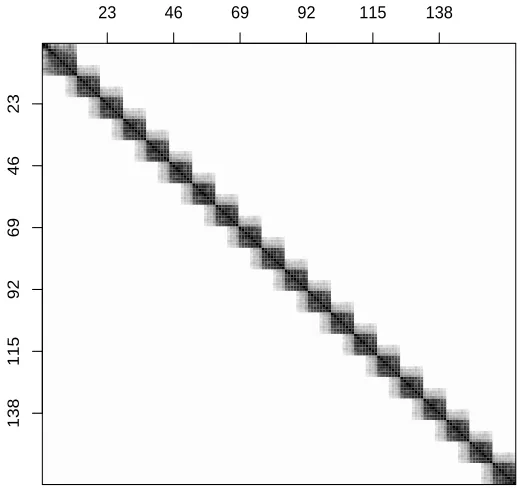
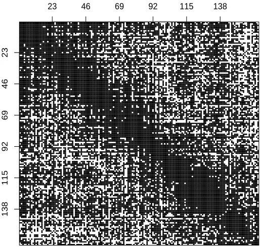
We now describe every step in detail by means of an example. Figure 1 gives the image of a partial correlation matrix for 164 variables. It is made up of 20 diagonal blocks of size 12×12 and there is a 4×4 submatrix overlap between every two adjacent blocks. The associated concentration graph, that we denote by G, has 1206 edges corresponding to 9% of all possible edges. We used this matrix as a concentration matrix to generate n=40 independent observations from a multivariate normal distribution with zero mean.
It is straightforward to check, by using the results of Section 4, that G(20)=G whereas G(3)is the complete graph and in this example we compare the qp-procedure for both q=3 and q=20.
23 46 69 92 115 138
138
115
92
69
46
23
Figure 1: Image of a partial correlation matrix for 164 variables. Every entry of the matrix is represented as a gray-scaled point between zero (white points) and±1 (black points).
Xj, the required statistical tests are computed for a large number of sets randomly sampled from
Q
i j according to a uniform distribution. In the example we are considering, the non-rejection rate is estimated by sampling 500 elements fromQ
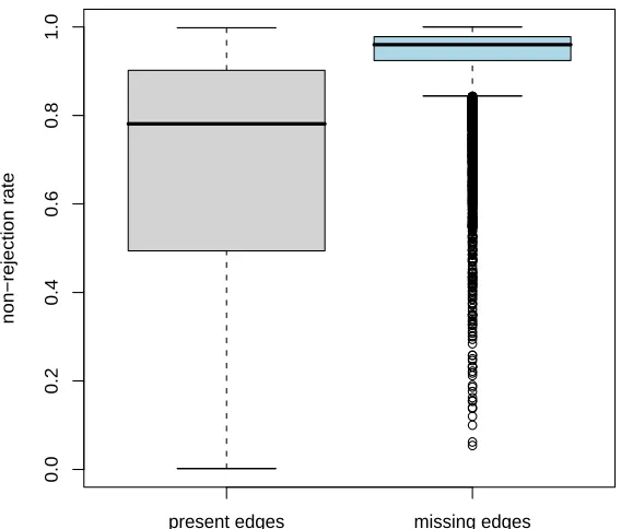
i j, for all of the 13 366 pairs of variables. For the case q=20, Figure 2 gives the boxplots of the estimates of the non-rejection rate for the present and missing edges of G(20). This picture provides a clear example of the different behavior of the non-rejection rate for present and missing edges and it is also worth recalling that that there is a large difference in the number of present and missing edges: 1206 versus 12 160.present edges missing edges
0.0
0.2
0.4
0.6
0.8
1.0
non−rejection rate
Figure 2: Boxplots of the estimated values of the non-rejection rate for the 1206 present edges and for the 12 160 missing edges of G=G(20).
dimensionality reduction. In particular, every circle below the dotted horizontal line corresponds to a model whose dimension is smaller than the sample size, and therefore that can be dealt with standard techniques.
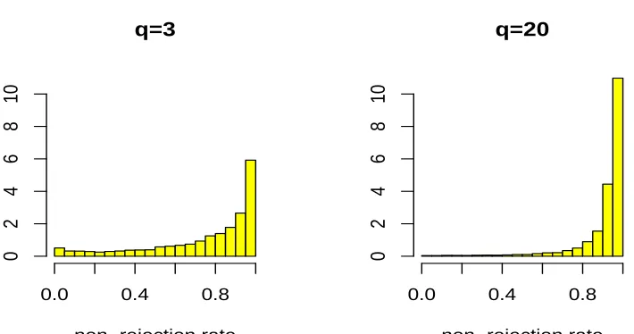
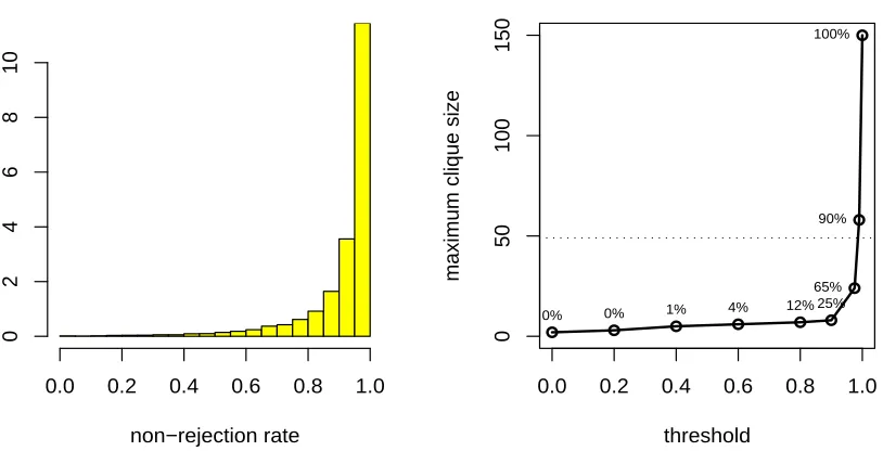
We now analyze these two types of plots for the example considered. Both histograms in Fig-ure 3 are asymmetric but the first histogram, for q=3, is less asymmetric with a heavier left tail, and this is a first indication that for the case q=3 the non-rejection rate may be of limited usefulness because we will not be able to remove many edges that are really missing without removing many others that should not be removed.
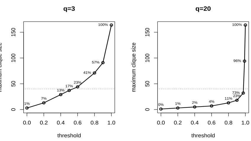
However, a more clear difference between the two cases can be derived from Figure 4. The dimension of models grows almost linearly for q=3 whereas, for the case q=20, it grows expo-nentially, increasing drastically only for threshold values larger than 0.975. For instance, for q=20, a threshold equal to 0.9 would lead to the removal of 77% of edges, returning a graph with 23% of edges left. The same threshold for q=3 would only lead to the removal of 43% of edges, returning a graph with 57% of edges left. Furthermore, the largest threshold that produces a graph for which the dimension of the largest clique is smaller than the sample size is 0.5 for q=3 and 0.975 for
q=3
non−rejection rate 0.0 0.4 0.8
0
2
4
6
8
10
q=20
non−rejection rate 0.0 0.4 0.8
0
2
4
6
8
10
Figure 3: Histograms of the estimated values of the non-rejection rates.
under analysis. For the case q=20 we can setβ∗=0.975 selecting in this way a graphGb(20)with 9751 out of 13 366 possible edges and whose largest clique has size 32. Figure 5 gives the adjacency matrix ofGb(20)and shows that, although this is clearly an overparameterized model, a substantial dimensionality reduction has been achieved while preserving the block diagonal structure of G(20).
Indeed, only 34 of the 1206 present edges are wrongly removed corresponding to an error of 2.8%.
5.3 Experimental Results
In this section we use simulated data to describe the behavior of the non-rejection rate for different values of q, n and different degrees of sparsity of the concentration graph. Furthermore, we present the application of the procedure to a real data set.
For the simulations, we set p=150 and constructed two graphs, G1= (V,E1)and G2= (V,E2) which have been randomly generated by imposing that every vertex has at most 5 and 20 adjacencies respectively. In this way, it follows from the results of Section 4 that for all q≥5 it holds that
G(1q)=G1 whereas for all q≥20 it holds that G( q)
2 =G2. The graph G1 has 375 edges whereas
G2has 1499 edges that correspond to 3.36% and 13.4% of the 11 175 possible edges respectively. Successively, an inverse covariance matrix with the zero pattern induced by G1has been randomly constructed (see Roverato, 2002) and then two samples, of size 20 and 150 respectively, have been randomly generated from a normal distribution with zero mean and the given covariance matrix. The same procedure was used to generate two random samples of size 20 and 50 for G2.
We first consider G1 and n=20 and independently apply the qp-procedure with six different values of q, ranging from 1 to 17; recall that the latter is the maximum possible value of q when
0.0 0.2 0.4 0.6 0.8 1.0
0
50
100
150
q=3
threshold
maximum clique size
1% 7%
13% 17%
23% 41%
57% 100%
0.0 0.2 0.4 0.6 0.8 1.0
0
50
100
150
q=20
threshold
maximum clique size
0% 1% 2% 4%
11%23% 73% 96% 100%
Figure 4: Plots giving the largest clique sizes of the graphs selected with different threshold values. For every graph the percentage of present edges is given and the dotted horizontal line is the sample size n.
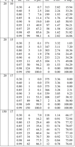
non-rejection rate is very high for all pairs of variables. As the value of(n−q)increases the qp-hist plots show heavier left tails while maintaining a strong negative asymmetric form. As Figure 7 clarifies, this happens because the distributions of the non-rejection rate for present and missing edges become more and more separated as(n−q)increases. We remark that the present and missing edges in Figure 7 are relative to G1and not to G(1q).
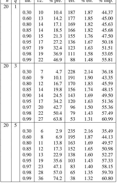
A numerical description of the results of these simulations is given in Tables 1 and 2. The first part of these tables gives the quantities used in the construction of the qp-clique plots: some threshold values (thr.) and, for every threshold, the size of the largest clique (l.c.) and the percentage of present edges (% pre.) of the corresponding graph. The remaining columns provide measures of goodness of the graph associated with each threshold. More specifically, “err.” gives the number of wrongly removed edges, “% err.” is the percentage of wrongly removed edges with respect to all the removed edges and, finally, “% imp.” is the rate of improvement with respect to the random removal of edges: a learning procedure based on the random removal of edges would lead to a relative error whose expected value is the proportion of edges in the graph, that is 3.36% for G1, and the improvement rate of a graph is the relative difference between “% err.” and the proportion of present edges in the concentration graph. We remark that the last three columns of these tables are not available in real applications where the concentration graph is unknown.
23 46 69 92 115 138
138
115
92
69
46
23
Figure 5: Adjacency matrix of the graph selected by the qp-procedure with q=20 andβ∗=0.975. Black points are present edges (value 1 in the adjacency matrix) and white points missing edges (value 0 in the adjacency matrix).
guarantee an adequate sparseness of G(1q). If in Tables 1 and 2 one takes, for the different values of q and n=20, the largest threshold corresponding to a graph whose largest clique size is smaller than
n, then the best solution is provided by q=10 with a graph in which 6601 edges are missing, the
largest clique has size 13 and the absolute error is 97 with a 56.21% improvement rate. However,
also the case q=5 provides a good solution with a graph in which 7194 edges are missing, the
largest clique has size 19 and the absolute error is 103 with a 57.33% improvement rate. A value of
q equal either to 5 or to 10 represents the most natural choice in the trade-off between(n−q)and
(p−q)in (6), however we notice that, apart from q=17 where the relative improvement is only 38.32%, all the other considered values of q provide satisfying solutions. This seems to suggest that the qp-procedure is not very sensitive to the choice of q. We can conclude that the qp-procedure is very effective despite the fact that we are considering an extremely challenging problem where the sample size is very small, n=20, compared to the number of variables, p=150. In order to show the behavior of the non-rejection rate as the sample size increases, in Figure 8 and Table 2
we provide an example in which the sample size is larger, n=150, but still too low to permit
n q thr. l.c. % pre. err. % err. % imp. 20 1
0.30 10 10.4 187 1.87 44.37 0.60 13 14.2 177 1.85 45.00 0.80 14 17.1 169 1.82 45.63 0.85 14 18.5 166 1.82 45.68 0.90 15 21.3 155 1.76 47.50 0.95 17 27.2 136 1.67 50.18 0.97 19 32.4 123 1.63 51.51 0.98 19 36.9 111 1.58 53.05 0.99 22 46.9 88 1.48 55.81 20 3
0.30 7 4.7 228 2.14 36.18 0.60 9 10.1 191 1.90 43.35 0.80 12 16.7 170 1.83 45.59 0.85 14 19.8 156 1.74 48.15 0.90 14 24.5 143 1.69 49.50 0.95 17 34.2 120 1.63 51.36 0.97 20 42.7 96 1.50 55.36 0.98 22 50.4 79 1.43 57.49 0.99 27 63.8 53 1.31 60.99 20 5
0.30 6 2.9 235 2.16 35.49 0.60 8 6.9 195 1.87 44.13 0.80 11 13.8 163 1.69 49.57 0.85 12 17.3 152 1.65 50.98 0.90 13 22.9 138 1.60 52.27 0.95 19 35.6 103 1.43 57.33 0.97 23 47.1 83 1.40 58.15 0.98 28 57.0 65 1.35 59.70 0.99 36 74.2 38 1.32 60.80
n q thr. l.c. % pre. err. % err. % imp. 20 10
0.30 4 0.7 313 2.82 15.94 0.60 5 2.5 244 2.24 33.26 0.80 7 7.6 199 1.93 42.59 0.85 8 11.4 174 1.76 47.66 0.90 9 19.0 149 1.65 50.93 0.95 13 40.9 97 1.47 56.21 0.97 25 67.2 58 1.58 52.83 0.98 45 85.6 26 1.62 51.82 0.99 99 98.1 6 2.82 16.06 20 15
0.30 2 0.1 371 3.32 1.03 0.60 3 0.3 347 3.11 7.20 0.80 5 1.0 303 2.74 18.36 0.85 6 1.9 278 2.54 24.45 0.90 6 5.5 233 2.21 34.28 0.95 11 45.5 104 1.71 49.08 0.97 50 94.2 10 1.53 54.29 0.98 124 99.6 0 0.00 100.00 0.99 150 100.0 0 0.00 100.00 20 17
0.30 1 0.0 375 3.36 0.00 0.60 1 0.0 375 3.36 0.00 0.80 1 0.0 375 3.36 0.00 0.85 2 0.1 366 3.28 2.31 0.90 3 0.4 339 3.05 9.23 0.95 11 53.3 108 2.07 38.32 0.97 89 98.7 2 1.38 58.90 0.98 149 99.9 0 0.00 100.00 0.99 150 100.0 0 0.00 100.00 150 17
0.30 6 7.0 118 1.14 66.17 0.60 9 16.2 85 0.91 72.94 0.80 13 29.4 60 0.76 77.32 0.85 15 35.6 53 0.74 78.07 0.90 17 44.3 44 0.71 78.93 0.95 23 60.4 34 0.77 77.10 0.97 34 70.7 30 0.92 72.72 0.98 44 77.5 21 0.84 75.09 0.99 62 86.3 12 0.78 76.61
q = 17
0.0 0.2 0.4 0.6 0.8 1.0
0
5
10
15
20
25
30
q = 15
0.0 0.2 0.4 0.6 0.8 1.0
0
5
10
15
20
q = 10
0.0 0.2 0.4 0.6 0.8 1.0
0
5
10
15
q = 5
0.0 0.2 0.4 0.6 0.8 1.0
0
5
10
15
q = 3
0.0 0.2 0.4 0.6 0.8 1.0
0
5
10
15
q = 1
0.0 0.2 0.4 0.6 0.8 1.0
0
5
10
15
Figure 6: qp-hist plots for G1= (V,E1)with n=20.
We now apply the qp-procedure for the case with concentration graph G2, n=20,50 and q= 5,10; see Figure 9 and Table 3. The graph G2is not sparse and both G(25)and G(210)are even more dense, and this affects the shape of the qp-hist plots in Figure 9. Indeed, all the three histograms are clearly less asymmetric than the corresponding histograms in Figure 6; note also that this is less evident in the case n=20 and q=10 because the quantity(n−q)is smaller than in the other two cases.
We deem that this kind of behavior of the qp-hist plot should be read as an indication that the considered q-partial graphs do not provide satisfying approximations of the required concentration graphs. Hence, if the value of q cannot be increased then we suggest that the application of any learning procedure based on limited-order partial correlations should be avoided for the problem under analysis.
We close this section applying the qp-procedure to a subset of the gene expression data from the study by West et al. (2001). This subset was extracted and analysed originally by Jones et al. (2005) and contains the expression profiles for p=150 genes associated with the estrogen receptor
pathway coming from n=49 breast tumor samples.
We have applied the qp-procedure with q=20 and the qp-hist and qp-clique plots, given in
present edges missing edges 0.0 0.2 0.4 0.6 0.8 1.0
q = 17
present edges missing edges
0.0 0.2 0.4 0.6 0.8 1.0
q = 15
present edges missing edges
0.0 0.2 0.4 0.6 0.8 1.0
q = 10
present edges missing edges
0.0 0.2 0.4 0.6 0.8 1.0
q = 5
present edges missing edges
0.0 0.2 0.4 0.6 0.8 1.0
q = 3
present edges missing edges
0.0 0.2 0.4 0.6 0.8 1.0
q = 1
Figure 7: Distribution of the non-rejection rate for present and missing edges of G1= (V,E1), to be associated with the corresponding histograms in Figure 6.
q = 17
0.0 0.2 0.4 0.6 0.8 1.0
0
2
4
6
8
present edges missing edges
0.0 0.2 0.4 0.6 0.8 1.0
q = 17
Figure 8: qp-hist plot and associated distributions of the non-rejection rate for present and missing edges of G1= (V,E1), resulting from the application of the qp-procedure where n=150
and q=17.
n = 20, q = 5
0.0 0.2 0.4 0.6 0.8 1.0
0
1
2
3
n = 20, q = 10
0.0 0.2 0.4 0.6 0.8 1.0
0
2
4
6
8
n = 50, q = 10
0.0 0.2 0.4 0.6 0.8 1.0
0
1
2
3
Figure 9: qp-hist plots and associated distributions of the non-rejection rate for present and missing edges of G2= (V,E2), resulting from the application of the qp-procedure for different values of n and q.
the dimension of the data. Such a feature may be a critical piece of information when dealing with real data for which we lack background knowledge on its underlying structure of interactions.
non−rejection rate
0.0 0.2 0.4 0.6 0.8 1.0
0
2
4
6
8
10
0.0 0.2 0.4 0.6 0.8 1.0
0
50
100
150
threshold
maximum clique size
0% 0% 1% 4% 12% 25% 65%
90% 100%
n q thr. l.c. % pre. err. % err. % imp. 20 5
0.30 5 3.6 1342 12.45 6.78 0.60 10 15.7 1099 11.66 12.72 0.80 21 40.8 735 11.11 16.82 0.85 29 54.2 580 11.33 15.16 0.90 55 72.9 328 10.84 18.89 0.95 103 91.6 90 9.59 28.18 0.97 123 96.5 31 7.81 41.55 0.98 134 98.3 23 12.30 7.94 0.99 144 99.5 6 10.00 25.15 20 10
0.30 3 0.5 1451 13.05 2.36 0.60 5 2.8 1333 12.27 8.13 0.80 7 11.9 1094 11.12 16.77 0.85 9 19.5 971 10.80 19.19 0.90 12 34.3 758 10.32 22.72 0.95 43 73.1 292 9.69 27.44 0.97 88 92.4 76 8.91 33.31 0.98 116 97.8 20 8.16 38.90 0.99 141 99.7 2 6.90 48.38 50 10
0.30 6 6.0 1171 11.14 16.59 0.60 9 21.4 869 9.89 25.96 0.80 17 49.2 518 9.13 31.69 0.85 27 64.3 351 8.79 34.20 0.90 62 82.8 152 7.91 40.81 0.95 120 96.9 27 7.87 41.08 0.97 134 99.4 7 9.59 28.23 0.98 143 99.8 3 12.50 6.44 0.99 148 100.0 0 0.00 100.00
Table 3: Graph G2= (V,E2). Numerical description of the output of the qp-procedure applied for different values of n and q. See Table 1 for a description of columns.
6. Discussion
This paper provides two main contributions: the theory related to q-partial graphs and the qp-procedure.
The theory of q-partial graphs clarifies the connection between the sparseness of the concentra-tion graph and the usefulness of marginal distribuconcentra-tions in structure learning, under the assumpconcentra-tion of faithfulness.
lack of faithfulness has a very weak impact on the resulting estimate. Apart from faithfulness, the
qp-procedure does not require any additional assumptions with respect to traditional structure
learn-ing procedures and, in particular, the sparseness of the concentration graph, despite belearn-ing crucial for the effectiveness of the procedure, is not assumed but exploited when present. In the case the
qp-hist and qp-clique plots provide and indication that the concentration graph is not sparse, then
this should be read as a warning on the real usefulness of limited-order partial correlations in the problem under analysis. The fact that the qp-procedure is designed to select an overparameterized model might be regarded as a limitation, but in fact we deem that this is a useful feature that adds additional flexibility in its use. Indeed, the qp-procedure can be used as an explorative tool to assess the sparseness of the concentration graph and, therefore, the usefulness of q-partial correlations in structure learning. Furthermore, the result of the procedure may be applied to obtain a shrinkage estimate of the covariance matrix useful both in the case n is larger, but close, to p and in the case n is smaller than p. Finally, the set of all the submodels of the selected model may identify a restricted search space where a traditional structure learning procedure, either in a Bayesian or in a frequentist approach to inference, can be applied. In Gaussian graphical models it is assumed that XV follows a multivariate normal distribution, and the normality of microarray data is a disputed question. We refer to Wit and McClure (2004; Section 6.2.2) for a discussion of this point, but we remark that the non-rejection rate is a quantity that can be obtained from any test for conditional independence computed on marginal distributions, and therefore it constitutes a general tool that can be used also outside the multivariate normal case.
The qp-procedure, jointly with other functions showing the qp-hist and qp-clique plots, has been implemented in a package, named qp, for the statistical software R (http://www.r-project.org).
This package can be downloaded from The Comprehensive R Archive Network (CRAN) athttp:
//cran.r-project.org/src/contrib/PACKAGES.html.
The qp-procedure is implemented in this package through the R and C programming languages requiring 10 minutes in a laptop 1.33GHz PowerPC G4 with 1.25 Gbyte RAM running Mac OS X, as well as in a desktop Intel 1.60GHz P4 with 1 Gbyte RAM running Linux, to perform the calculations of one of the simulations involving p=150 variables, n=50 observations, and q= 15 sampling 500 conditioning subsets to estimate the non-rejection rate for each of the 11 175 adjacencies. Note also that the p×(p−1)/2 non-rejection rates could be estimated in parallel and thus such an implementation would greatly improve the performance.
Acknowledgments
Appendix A. Graph Theory
In this appendix we present the graph theory required for this paper and, in particular, we introduce the novel concept of outer connectivity that is used in Section 4 to describe the properties of q-partial graphs. We refer to Cowell et al. (1999) for a full account of graph theory usually applied in graphical models, to Diestel (2005) for the theory relating separators and independent paths and, finally, to Rosenberg and Heath (2005) for a comprehensive description of the techniques for obtaining upper and lower bounds on the sizes of graph separators.
An undirected graph is a pair G= (V,E), where V ={1, . . . ,p}is a finite set of vertices and in this paper E, called the edge set, is a subset of the set of unordered distinct pair of vertices. If two vertices i,j∈V form an edge then we say that i and j are adjacent and write(i,j)∈E; recall
that edges are unordered pairs, so that(i,j) = (j,i). Graphs are usually represented by drawing a dot for each vertex and joining two of these dots by a line if the corresponding two vertices form
an edge; see Figure 11 for a few examples. For a subset A⊆V the subgraph of G induced by A
is GA= (A,EA)with EA=E∩(A×A). For two graphs with common vertex set, G= (V,E)and
G0= (V,E0), we say that G0 is larger than G, and write G⊆G0, if E ⊆E0; when the inclusion is strict, that is, E ⊂E0, we write G⊂G0 . The boundary of a vertex v∈V , denoted by bdG(v), is the set of vertices adjacent to v. A subset C⊆V with all vertices being mutually adjacent is called
complete, and when V is complete then we say that G is complete. A subset C⊆V is called a
clique if it is maximally complete, that is, C is complete, and if C⊂D, then D is not complete. An
undirected graph can be identified by the set
C
of its cliques. The set ¯E is the set of missing edges of G; that is, for a pair i,j∈V ,(i,j)∈E if and only if i¯ 6= j and(i,j)6∈E. A path of length l>0 fromv0 to vl is a sequence v0,v1, . . . ,vl of distinct vertices such that (vk−1,vk)∈E for all k=1, . . . ,l. Two or more paths from v0to vlare independent if they have no common vertices other then v0and
vl. We can define an equivalence relation on V as
i∼p j⇔ there is a path v0,v1, . . . ,vl with v0=i,vl= j.
The subgraphs induced by the equivalence classes are the connected components of G. If there is only one equivalence class, we say that G is connected. The subset U ⊆V is said to separate I⊆V
from J⊆V if for every i∈I and j∈J all paths from i to j have at least one vertex in U . For a
pair of vertices i6= j with(i,j)∈E, a set U¯ ⊆V is called a{i,j}-separator if it separates{i}and
{j}in G. If either i∈U or j∈U then we say that U is trivial. If no proper subset of U is a{i,j} -separator we say that U is minimal; see also Cowell et al. (1999). Note that the unique possible minimal {i,j}-separators that are trivial are {i} and {j}. Hereafter, to stress that a separator is nontrivial and minimal we denote it by S; furthermore, we denote by
S
(i,j|G)the set of all nontrivial minimal{i,j}-separators in G, so thatS
(i,j|G)={/0}if and only if i and j are in different connectedcomponents. There is a close connection between the concepts of connectivity and separation: the dimension of the smallest{i,j}-separator, that is the cardinality of the smallest (possibly non unique) set in
S
(i,j|G), is called the connectivity of i and j because it represents both the maximumDefinition 3 Let i6= j be a pair vertices of an undirected graph G= (V,E). The outer connectivity
of i and j is defined as
d(i,j|G) = min
S∈S(i,j|Gi j) |S|
where Gi j is the graph with vertex set V and edge set Ei j=E\{(i,j)}.
Hence, d(i,j|G)is the connectivity of i and j in Gi j. The latter graph is constructed by removing the edge(i,j)from G, so that if(i,j)∈E then G¯ =Gi j. The idea here is that the edge(i,j)represents an
inner, or direct, connection between i and j and it should not be considered when outer, or indirect,
connectivity is of concern.
Example 1 For the vertex set V ={1, . . . ,6}let Gi= (V,Ei), i=1, . . . ,3 be the graphs in Figure
11 and let G4be the complete graph. Then
• d(2,3|Gi) =0 for i=1,2,3 whereas d(2,3|G4) =4;
• d(1,6|G1) =0, d(1,6|Gi) =1 for i=2,3 whereas d(1,6|G4) =4;
• d(3,4|Gi) =0 for i=1,2 whereas d(3,4|G3) =1;
• d(3,6|G1) =0, d(3,6|G2) =1, d(3,6|G3) =2.
PSfrag replacements
1 2 3 4 5 6 G1
PSfrag replacements
1 2 3 4 5 6 G2
PSfrag replacements
1 2 3
4
5
6 G3
Figure 11: Examples of undirected graph.
Computing the connectivity of two vertices is known to be a NP-hard problem, however several algorithms are available to derive both upper and lower bounds to this number; see Rosenberg and Heath (2001). Here we remark that the cardinality of any{i,j}-separator in Gi j is an upper bound to the connectivity of i and j; consequently, since bdGi j(i)and bdGi j(j)are both{i,j}-separators in
Gi j, then the number
e
d(i,j|G):=min{|bdGi j(i)|,|bdGi j(j)|} (7)
provides an easy-to-compute upper bound to the outer connectivity of i and j; formally
d(i,j|G)≤de(i,j|G) for all i,j∈V ; i6= j. (8)
It is useful to consider separately the pairs of vertices that define an edge in G from the pairs of vertices that are not adjacent in G. Hence, we define the outer connectivity of the edges of G= (V,E) as
d(E|G):= max