Spectral Learning of Latent-Variable PCFGs: Algorithms
and Sample Complexity
Shay B. Cohen [email protected]
School of Informatics University of Edinburgh Edinburgh, EH8 9LE, UK
Karl Stratos [email protected]
Michael Collins [email protected]
Department of Computer Science Columbia University
New York, NY 10027, USA
Dean P. Foster [email protected]
Yahoo! Labs
New York, NY 10018, USA
Lyle Ungar [email protected]
Department of Computer and Information Science University of Pennsylvania
Philadelphia, PA 19104, USA
Editor:Alexander Clark
Abstract
We introduce a spectral learning algorithm for latent-variable PCFGs (Matsuzaki et al., 2005; Petrov et al., 2006). Under a separability (singular value) condition, we prove that the method provides statistically consistent parameter estimates. Our result rests on three theorems: the first gives a tensor form of the inside-outside algorithm for PCFGs; the second shows that the required tensors can be estimated directly from training examples where hidden-variable values are missing; the third gives a PAC-style convergence bound for the estimation method.
Keywords: latent-variable PCFGs, spectral learning algorithms
1. Introduction
Recent work has introduced a polynomial-time learning algorithm for an important case of hidden-variable models: hidden Markov models (Hsu et al., 2009). This algorithm uses a spectral method: that is, an algorithm based on eigenvector decompositions of linear systems, in particular singular value decomposition (SVD). In the general case, learning of HMMs is intractable (e.g., see Terwijn, 2002). The spectral method finesses the prob-lem of intractability by assuming separability conditions. More precisely, the algorithm of Hsu et al. (2009) has a sample complexity that is polynomial in 1{σ, where σ is the mini-mum singular value of an underlying decomposition. The HMM learning algorithm is not susceptible to problems with local maxima.
In this paper we derive a spectral algorithm for learning of latent-variable PCFGs (L-PCFGs) (Petrov et al., 2006; Matsuzaki et al., 2005). L-PCFGs have been shown to be a very effective model for natural language parsing. Under a condition on singular values in the underlying model, our algorithm provides consistent parameter estimates; this is in contrast with previous work, which has used the EM algorithm for parameter estimation, with the usual problems of local optima.
The parameter estimation algorithm (see Figure 7) is simple and efficient. The first step is to take an SVD of the training examples, followed by a projection of the training examples down to a low-dimensional space. In a second step, empirical averages are calculated on the training examples, followed by standard matrix operations. On test examples, tensor-based variants of the inside-outside algorithm (Figures 4 and 5) can be used to calculate probabilities and marginals of interest.
Our method depends on the following results:
• Tensor form of the inside-outside algorithm. Section 6.1 shows that the inside-outside algorithm for L-PCFGs can be written using tensors and tensor products. Theorem 3 gives conditions under which the tensor form calculates inside and outside terms correctly.
• Observable representations. Section 7.2 shows that under a singular-value condition, there is an observable form for the tensors required by the inside-outside algorithm. By an observable form, we follow the terminology of Hsu et al. (2009) in referring to quantities that can be estimated directly from data where values for latent variables are unobserved. Theorem 6 shows that tensors derived from the observable form satisfy the conditions of Theorem 3.
• Estimating the model. Section 8 gives an algorithm for estimating parameters of the observable representation from training data. Theorem 8 gives a sample complexity result, showing that the estimates converge to the true distribution at a rate of 1{?M whereM is the number of training examples.
In this paper we derive the basic algorithm, and the theory underlying the algorithm. In a companion paper (Cohen et al., 2013), we describe experiments using the algorithm to learn an L-PCFG for natural language parsing. In these experiments the spectral algorithm gives models that are as accurate as the EM algorithm for learning in L-PCFGs. It is significantly more efficient than the EM algorithm on this problem (9h52m of training time vs. 187h12m), because after an SVD operation it requires a single pass over the data, whereas EM requires around 20-30 passes before converging to a good solution.
2. Related Work
The most common approach for statistical learning of models with latent variables is the expectation-maximization (EM) algorithm (Dempster et al., 1977). Under mild conditions, the EM algorithm is guaranteed to converge to a local maximum of the log-likelihood function. This is, however, a relatively weak guarantee; there are in general no guarantees of consistency for the EM algorithm, and no guarantees of sample complexity, for example within the PAC framework (Valiant, 1984). This has led a number of researchers to consider alternatives to the EM algorithm, which do have PAC-style guarantees.
One focus of this work has been on the problem of learning Gaussian mixture models. In early work, Dasgupta (1999) showed that under separation conditions for the underlying Gaussians, an algorithm with PAC guarantees can be derived. For more recent work in this area, see for example Vempala and Wang (2004), and Moitra and Valiant (2010). These algorithms avoid the issues of local maxima posed by the EM algorithm.
Another focus has been on spectral learning algorithms for hidden Markov models (HMMs) and related models. This work forms the basis for the L-PCFG learning algo-rithms described in this paper. This line of work started with the work of Hsu et al. (2009), who developed a spectral learning algorithm for HMMs which recovers an HMM’s param-eters, up to a linear transformation, using singular value decomposition and other simple matrix operations. The algorithm builds on the idea of observable operator models for HMMs due to Jaeger (2000). Following the work of Hsu et al. (2009), spectral learning algorithms have been derived for a number of other models, including finite state transduc-ers (Balle et al., 2011); split-head automaton grammars (Luque et al., 2012); reduced rank HMMs in linear dynamical systems (Siddiqi et al., 2010); kernel-based methods for HMMs (Song et al., 2010); and tree graphical models (Parikh et al., 2011; Song et al., 2011). There are also spectral learning algorithms for learning PCFGs in the unsupervised setting (Bailly et al., 2013).
Foster et al. (2012) describe an alternative algorithm to that of Hsu et al. (2009) for learning of HMMs, which makes use of tensors. Our work also makes use of tensors, and is closely related to the work of Foster et al. (2012); it is also related to the tensor-based approaches for learning of tree graphical models described by Parikh et al. (2011) and Song et al. (2011). In related work, Dhillon et al. (2012) describe a tensor-based method for dependency parsing.
corresponding to larger tree fragments. Cohen et al. (2013) give definitions of φ and ψ used in parsing experiments with L-PCFGs. In the special case whereφand ψare identity functions, specifying the entire inside or outside tree, the learning algorithm of Bailly et al. (2010) is the same as our algorithm. However, our work differs from that of Bailly et al. (2010) in several important respects. The generalization to allow arbitrary functionsφand ψis important for the success of the learning algorithm, in both a practical and theoretical sense. The inside-outside algorithm, derived in Figure 5, is not presented by Bailly et al. (2010), and is critical in deriving marginals used in parsing. Perhaps most importantly, the analysis of sample complexity, given in Theorem 8 of this paper, is much tighter than the sample complexity bound given by Bailly et al. (2010). The sample complexity bound in theorem 4 of Bailly et al. (2010) suggests that the number of samples required to obtain
|pˆptq ´pptq| ď for some tree t of size N, and for some value , is exponential in N. In contrast, we show that the number of samples required to obtainř
t|pˆptq ´pptq| ďwhere the sum is over alltrees of sizeN is polynomial in N. Thus our bound is an improvement in a couple of ways: first, it applies to a sum over all trees of size N, a set of exponential size; second, it is polynomial inN.
Spectral algorithms are inspired by the method of moments, and there are latent-variable learning algorithms that use the method of moments, without necessarily resorting to spec-tral decompositions. Most relevant to this paper is the work in Cohen and Collins (2014) for estimating L-PCFGs, inspired by the work by Arora et al. (2013).
3. Notation
Given a matrix A or a vector v, we write AJ or vJ for the associated transpose. For any integerně1, we usernsto denote the sett1,2, . . . nu.
We useRmˆ1 to denote the space ofm-dimensional column vectors, andR1ˆm to denote
the space of m-dimensional row vectors. We useRm to denote the space of m-dimensional
vectors, where the vector in question can be either a row or column vector. For any row or column vectory PRm, we use diagpyqto refer to thepmˆmqmatrix with diagonal elements
equal to yh for h“1. . . m, and off-diagonal elements equal to 0. For any statement Γ, we use vΓw to refer to the indicator function that is 1 if Γ is true, and 0 if Γ is false. For a random variableX, we use ErXs to denote its expected value.
We will make use of tensors of rank 3:
Definition 1 A tensor C P Rpmˆmˆmq is a set of m3 parameters Ci,j,k for i, j, k P rms. Given a tensor C, and vectors y1 P Rm and y2 P Rm, we define Cpy1, y2q to be the m
-dimensional row vector with components
rCpy1, y2qsi “
ÿ
jPrms,kPrms
Ci,j,kyj1yk2.
Hence C can be interpreted as a function C :RmˆRm Ñ R1ˆm that maps vectors y1 and
y2 to a row vector Cpy1, y2q PR1ˆm.
In addition, we define the tensor Cp1,2q PRpmˆmˆmq for any tensor C P Rpmˆmˆmq to
be the function Cp1,2q:RmˆRm ÑRmˆ1 defined as
rCp1,2qpy1, y2qsk“
ÿ
iPrms,jPrms
Similarly, for any tensor C we define Cp1,3q:RmˆRmÑRmˆ1 as
rCp1,3qpy1, y2qsj “
ÿ
iPrms,kPrms
Ci,j,kyi1yk2.
Note that Cp1,2qpy1, y2q andCp1,3qpy1, y2q are both columnvectors.
For vectors x, y, z PRm, xyJzJ is the tensor DPRmˆmˆm where Di,j,k “xiyjzk (this is analogous to the outer product: rxyJ
si,j “xiyj).
We use ||. . .||F to refer to the Frobenius norm for matrices or tensors: for a matrixA, ||A||F “
b ř
i,jpAi,jq2, for a tensor C, ||C||F “
b ř
i,j,kpCi,j,kq2. For a matrix A we use ||A||2,o to refer to the operator (spectral) norm,||A||2,o“maxx‰0||Ax||2{||x||2.
4. L-PCFGs
In this section we describe latent-variable PCFGs (L-PCFGs), as used for example by Matsuzaki et al. (2005) and Petrov et al. (2006). We first give the basic definitions for L-PCFGs, and then describe the underlying motivation for them.
4.1 Basic Definitions
An L-PCFG is an 8-tuple pN,I,P, m, n, t, q, πq where:
• N is the set of non-terminal symbols in the grammar. I Ă N is a finite set of in-terminals. P ĂN is a finite set of pre-terminals. We assume that N “IYP, and IXP “ H. Hence we have partitioned the set of non-terminals into two subsets. • rmsis the set of possible hidden states.
• rnsis the set of possible words.
• For all a P I, b P N, c P N, h1, h2, h3 P rms, we have a context-free rule aph1q Ñ
bph2q cph3q.
• For allaPP,hP rms,xP rns, we have a context-free rule aphq Ñx.
• For allaPI, b, cPN, andh1, h2, h3P rms, we have a parametertpaÑb c, h2, h3|h1, aq. • For allaPP,xP rns, and hP rms, we have a parameter qpaÑx|h, aq.
• For all a P I and h P rms, we have a parameter πpa, hq which is the probability of non-terminalapaired with hidden variable h being at the root of the tree.
Note that each in-terminal aPI is always the left-hand-side of a binary rule aÑ b c; and each pre-terminalaPP is always the left-hand-side of a ruleaÑx. Assuming that the non-terminals in the grammar can be partitioned this way is relatively benign, and makes the estimation problem cleaner.
For convenience we define the set of possible “skeletal rules” asR“ taÑb c:aPI, bP
S1 NP2 D3 the
N4 dog
VP5 V6 saw
P7 him
r1 “S Ñ NP VP r2 “NP Ñ D N r3 “D Ñ the r4 “N Ñ dog r5 “VP Ñ V P r6 “V Ñ saw r7 “P Ñ him
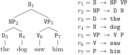
Figure 1: s-tree, and its sequence of rules. (For convenience we have numbered the nodes in the tree.)
These definitions give a PCFG, with rule probabilities
ppaph1q Ñbph2qcph3q|aph1qq “tpaÑb c, h2, h3|h1, aq, and
ppaphq Ñx|aphqq “qpaÑx|h, aq.
Remark 2 In the previous paper on this work (Cohen et al., 2012), we considered an L-PCFG model where
ppaph1q Ñbph2qcph3q|aph1qq “ppaÑb c|h1, aq ˆpph2|h1, aÑb cq ˆpph3|h1, aÑb cq
In this model the random variables h2 and h3 are assumed to be conditionally independent given h1 and aÑb c.
In this paper we consider a model where
ppaph1q Ñbph2qcph3q|aph1qq “tpaÑb c, h2, h3,|h1, aq. (1)
That is, we do not assume that the random variables h2 and h3 are independent when conditioning on h1 and aÑb c. This is also the model considered by Matsuzaki et al. (2005) and Petrov et al. (2006).
Note however that the algorithms in this paper are the same as those in Cohen et al. (2012): we have simply proved that the algorithms give consistent estimators for the model form in Eq. 1.
As in usual PCFGs, the probability of an entire tree is calculated as the product of its rule probabilities. We now give more detail for these calculations.
An L-PCFG defines a distribution over parse trees as follows. A skeletal tree (s-tree) is a sequence of rules r1. . . rN where each ri is either of the formaÑ b c or aÑ x. The rule sequence forms a top-down, left-most derivation under a CFG with skeletal rules. See Figure 1 for an example.
Define ai to be the non-terminal on the left-hand-side of rule ri. For any iP rNs such thatai PI (i.e.,aiis an in-terminal, and ruleri is of the formaÑb c) definehp2qi to be the hidden variable value associated with the left child of the ruleri, and hp3qi to be the hidden variable value associated with the right child. The probability mass function (PMF) over full trees is then
ppr1. . . rN, h1. . . hNq “πpa1, h1q ˆ
ź
i:aiPI
tpri, hp2qi , h p3q
i |hi, aiq ˆ
ź
i:aiPP
qpri|hi, aiq. (2)
The PMF over s-trees is ppr1. . . rNq “
ř
h1...hNppr1. . . rN, h1. . . hNq.
In the remainder of this paper, we make use of a matrix form of parameters of an L-PCFG, as follows:
• For eachaÑb cPR, we define TaÑb c
PRmˆmˆm to be the tensor with values
Tha1Ñ,hb c2,h3 “tpaÑb c, h2, h3|a, h1q.
• For eachaPP,xP rns, we define qaÑx PR1ˆm to be the row vector with values
rqaÑxsh “qpaÑx|h, aq forh“1,2, . . . m.
‚ For eachaPI, we define the column vector πaPRmˆ1 whererπash“πpa, hq.
4.2 Application of L-PCFGs to Natural Language Parsing
L-PCFGs have been shown to be a very useful model for natural language parsing (Mat-suzaki et al., 2005; Petrov et al., 2006). In this section we describe the basic approach.
We assume a training set consisting of sentences paired with parse trees, which are similar to the skeletal tree shown in Figure 1. A naive approach to parsing would simply read off a PCFG from the training set: the resulting grammar would have rules such as
S Ñ NP VP
NP Ñ D N
VP Ñ V NP
D Ñ the
N Ñ dog
and so on. Given a test sentence, the most likely parse under the PCFG can be found using dynamic programming algorithms.
Unfortunately, simple “vanilla” PCFGs induced from treebanks such as the Penn tree-bank (Marcus et al., 1993) typically give very poor parsing performance. A critical issue is that the set of non-terminals in the resulting grammar (S, NP, VP, PP, D, N, etc.) is often quite small. The resulting PCFG therefore makes very strong independence assump-tions, failing to capture important statistical properties of parse trees.
(Collins, 1997; Charniak, 1997), non-terminals such as S are replaced with non-terminals such asS-sleeps: the non-terminals track some lexical item (in this casesleeps), in addition to the syntactic category. For example, the parse tree in Figure 1 would include rules
S-saw Ñ NP-dog VP-saw
NP-dog Ñ D-the N-dog
VP-saw Ñ V-saw P-him
D-the Ñ the
N-dog Ñ dog
V-saw Ñ saw
P-him Ñ him
In this case the number of non-terminals in the grammar increases dramatically, but with appropriate smoothing of parameter estimates lexicalized models perform at much higher accuracy than vanilla PCFGs.
As another example, Johnson describes an approach where non-terminals are refined to also include the non-terminal one level up in the tree; for example rules such as
S Ñ NP VP
are replaced by rules such as
S-ROOT Ñ NP-S VP-S
Here NP-S corresponds to an NPnon-terminal whose parent is S;VP-S corresponds to a VP whose parent isS;S-ROOTcorresponds to an Swhich is at the root of the tree. This simple modification leads to significant improvements over a vanilla PCFG.
Klein and Manning (2003) develop this approach further, introducing annotations cor-responding to parents and siblings in the tree, together with other information, resulting in a parser whose performance is just below the lexicalized models of Collins (1997) and Charniak (1997).
The approaches of Collins (1997), Charniak (1997), Johnson, and Klein and Manning (2003) all use hand-constructed rules to enrich the set of non-terminals in the PCFG. A natural question is whether refinements to non-terminals can be learned automatically. Matsuzaki et al. (2005) and Petrov et al. (2006) addressed this question through the use of L-PCFGs in conjunction with the EM algorithm. The basic idea is to allow each non-terminal in the grammar to have m possible latent values. For example, with m “ 8 we would replace the non-terminal S with non-terminals S-1, S-2, . . ., S-8, and we would replace rules such as
S Ñ NP VP
with rules such as
S-4 Ñ NP-3 VP-2
be estimated using the EM algorithm. More specifically, given training examples consisting of skeletal trees of the formtpiq
“ pr1piq, rp2iq, . . . , rpNiq
iq, fori“1. . . M, whereNiis the number
of rules in thei’th tree, the log-likelihood of the training data is M
ÿ
i“1
logpprp1iq. . . rNpiq
iq “
M
ÿ
i“1
log ÿ h1...hNi
pprp1iq. . . rpNiq
i, h1. . . hNiq
where ppr1piq. . . rpNiq
i, h1. . . hNiq is as defined in Eq. 2. The EM algorithm is guaranteed to
converge to a local maximum of the log-likelihood function. Once the parameters of the L-PCFG have been estimated, the algorithm of Goodman (1996) can be used to parse test-data sentences using the L-PCFG: see Section 4.3 for more details. Matsuzaki et al. (2005) and Petrov et al. (2006) show very good performance for these methods.
4.3 Basic Algorithms for L-PCFGs: Variants of the Inside-Outside Algorithm Variants of the inside-outside algorithm (Baker, 1979) can be used for basic calculations in L-PCFGs, in particular for calculations that involve marginalization over the values for the hidden variables.
To be more specific, given an L-PCFG, two calculations are central:
1. For a given s-treer1. . . rN, calculateppr1. . . rNq “
ř
h1...hNppr1. . . rN, h1. . . hNq.
2. For a given input sentencex“x1. . . xN, calculate the marginal probabilities µpa, i, jq “
ÿ
τPTpxq:pa,i,jqPτ ppτq
for each non-terminal a P N, for each pi, jq such that 1 ď i ď j ď N. Here Tpxq
denotes the set of all possible s-trees for the sentence x, and we write pa, i, jq Pτ if non-terminalaspans words xi. . . xj in the parse tree τ.
The marginal probabilities have a number of uses. Perhaps most importantly, for a given sentencex“x1. . . xN, the parsing algorithm of Goodman (1996) can be used to find
arg max τPTpxq
ÿ
pa,i,jqPτ
µpa, i, jq.
This is the parsing algorithm used by Petrov et al. (2006), for example.1 In addition, we can calculate the probability for an input sentence, ppxq “ řτPTpxqppτq, as ppxq “
ř
aPIµpa,1, Nq.
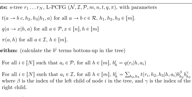
Figures 2 and 3 give the conventional (as opposed to tensor) form of inside-outside algorithms for these two problems. In the next section we describe the tensor form. The algorithm in Figure 2 uses dynamic programming to compute
ppr1. . . rNq “
ÿ
h1...hN
ppr1. . . rN, h1. . . hNq
1. Note that finding arg maxτPTpxqppτq, whereppτq “
ř
Inputs: s-tree r1. . . rN, L-PCFGpN,I,P, m, n, t, q, πq, with parameters • tpaÑb c, h2, h3|h1, aq for all aÑb cPR,h1, h2, h3 P rms.
• qpaÑx|h, aq for all aPP, xP rns, hP rms
• πpa, hq for all aPI,hP rms.
Algorithm: (calculate the bi terms bottom-up in the tree)
• For alliP rNssuch thataiPP, for all hP rms,bih“qpri|h, aiq
• For alliP rNssuch that ai PI, for allhP rms,bih “
ř
h2,h3tpri, h2, h3|h, aiqb β h2b
γ h3 whereβ is the index of the left child of nodeiin the tree, andγ is the index of the right child.
Return: řhb1hπpa1, hq “ppr1. . . rNq
Figure 2: The conventional inside-outside algorithm for calculation of ppr1. . . rNq.
for a given parse tree r1. . . rN. The algorithm in Figure 3 uses dynamic programming to compute marginal terms.
5. Roadmap
The next three sections of the paper derive the spectral algorithm for learning of L-PCFGs. The structure of these sections is as follows:
• Section 6 introduces atensor formof the inside-outside algorithms for L-PCFGs. This is analogous to the matrix form for hidden Markov models (see Jaeger 2000, and in particular Lemma 1 of Hsu et al. 2009), and is also related to the use of tensors in spectral algorithms for directed graphical models (Parikh et al., 2011).
• Section 7.2 derives anobservable form for the tensors required by algorithms of Sec-tion 6. The implicaSec-tion of this result is that the required tensors can be estimated directly from training data consisting of skeletal trees.
• Section 8 gives the algorithm for estimation of the tensors from a training sample, and gives a PAC-style generalization bound for the approach.
6. Tensor Form of the Inside-Outside Algorithm
This section first gives a tensor form of the inside-outside algorithms for L-PCFGs, then give an illustrative example.
6.1 The Tensor-Form Algorithms
Inputs: Sentence x1. . . xN, L-PCFGpN,I,P, m, n, t, q, πq, with parameters • tpaÑb c, h2, h3|h1, aq for all aÑb cPR,h1, h2, h3 P rms.
• qpaÑx|h, aq for all aPP, xP rns, hP rms
• πpa, hq for all aPI,hP rms. Data structures:
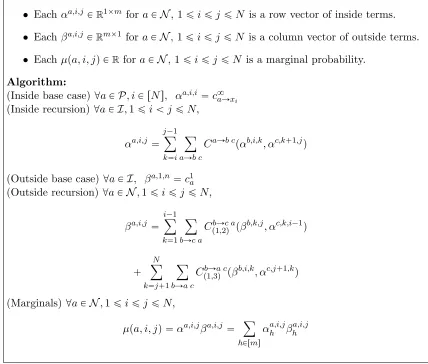
• Each ¯αa,i,j P
R1ˆm foraPN, 1ďiďj ďN is a row vector of inside terms.
• Each ¯βa,i,j PRmˆ1 foraPN, 1ďiďjďN is a column vector of outside terms.
• Each ¯µpa, i, jq PRforaPN, 1ďiďjďN is a marginal probability. Algorithm:
(Inside base case)@aPP, iP rNs, hP rms α¯a,i,ih “qpaÑxi|h, aq (Inside recursion)@aPI,1ďiăjďN, hP rms
¯ αa,i,jh “
j´1 ÿ
k“i
ÿ
aÑb c
ÿ
h2Prms ÿ
h3Prms
tpaÑb c, h2, h3|h, aq ˆα¯b,i,kh 2 ˆα¯
c,k`1,j h3
(Outside base case) @aPI, hP rms β¯ha,1,n “πpa, hq
(Outside recursion) @aPN,1ďiďjďN, hP rms
¯ βha,i,j “
i´1 ÿ
k“1 ÿ
bÑc a
ÿ
h2Prms ÿ
h3Prms
tpbÑc a, h3, h|h2, bq ˆβ¯hb,k,j2 ˆα¯c,k,ih3 ´1
` N
ÿ
k“j`1 ÿ
bÑa c
ÿ
h2Prms ÿ
h3Prms
tpbÑa c, h, h3|h2, bq ˆβ¯hb,i,k2 ˆα¯ c,j`1,k h3
(Marginals)@aPN,1ďiďjďN,
¯
µpa, i, jq “α¯a,i,jβ¯a,i,j “ ÿ hPrms
¯
αa,i,jh β¯ha,i,j
Inputs: s-tree r1. . . rN, L-PCFGpN,I,P, m, nq, parameters • CaÑb c
PRpmˆmˆmq for all aÑb cPR
• c8
aÑx PRp1ˆmq for all aPP, xP rns • c1aPRpmˆ1q for all aPI.
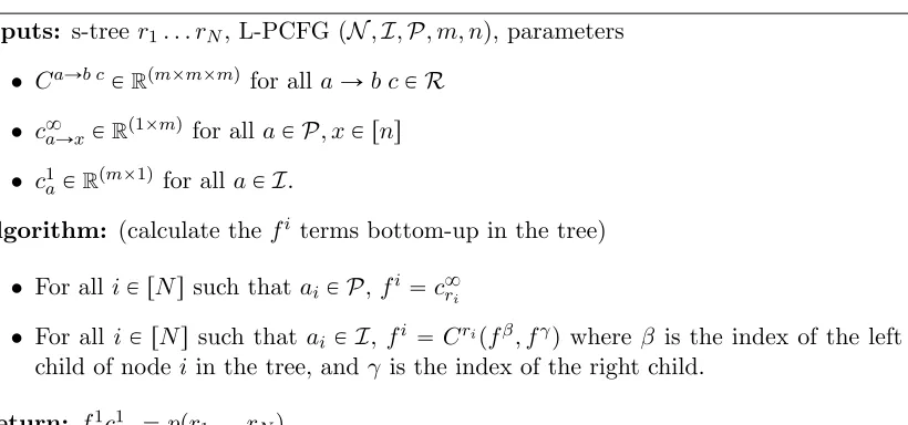
Algorithm: (calculate the fi terms bottom-up in the tree) • For alliP rNssuch thataiPP,fi “c8ri
• For all iP rNs such that ai PI,fi “Cripfβ, fγq where β is the index of the left child of nodeiin the tree, and γ is the index of the right child.
Return: f1c1a1 “ppr1. . . rNq
Figure 4: The tensor form for calculation of ppr1. . . rNq.
1. For a given s-treer1. . . rN, calculateppr1. . . rNq.
2. For a given input sentencex“x1. . . xN, calculate the marginal probabilities µpa, i, jq “ ÿ
τPTpxq:pa,i,jqPτ ppτq
for each non-terminal a P N, for each pi, jq such that 1 ď i ď j ď N, where Tpxq
denotes the set of all possible s-trees for the sentence x, and we write pa, i, jq Pτ if non-terminalaspans words xi. . . xj in the parse tree τ.
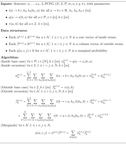
The tensor form of the inside-outside algorithms for these two problems are shown in Figures 4 and 5. Each algorithm takes the following inputs:
1. A tensor CaÑb c
PRpmˆmˆmq for each rule aÑb c. 2. A vector c8
aÑx PRp1ˆmq for each rule aÑx.
3. A vector c1
aPRpmˆ1q for each aPI.
The following theorem gives conditions under which the algorithms are correct:
Theorem 3 Assume that we have an L-PCFG with parametersqaÑx, TaÑb c,πa, and that there exist matrices Ga P Rpmˆmq for all aP N such that each Ga is invertible, and such
that:
1. For all rules aÑb c,CaÑb c
py1, y2q “`TaÑb c
py1Gb, y2Gcq˘pGaq´1. 2. For all rules aÑx, c8
Then: 1) The algorithm in Figure 4 correctly computes ppr1. . . rNq under the L-PCFG. 2) The algorithm in Figure 5 correctly computes the marginals µpa, i, jq under the L-PCFG.
Proof: see Section A.1. The next section (Section 6.2) gives an example that illustrates
the basic intuition behind the proof.
Remark 4 It is easily verified (see also the example in Section 6.2), that if the inputs to the tensor-form algorithms are of the following form (equivalently, the matrices Ga for all a are equal to the identity matrix):
1. For all rules aÑb c,CaÑb cpy1, y2q “TaÑb cpy1, y2q. 2. For all rules aÑx, c8
aÑx“qaÑx. 3. For all aPI, c1
a“πa.
then the algorithms in Figures 4 and 5 are identical to the algorithms in Figures 2 and 3 respectively. More precisely, we have the identities
bih“fhi for the quantities in Figures 2 and 4, and
¯
αa,i,jh “αa,i,jh ¯
βa,i,jh “βha,i,j for the quantities in Figures 3 and 5.
The theorem shows, however, that it is sufficient2 to have parameters that are equal to TaÑb c,q
aÑxandπaup to linear transforms defined by the matricesGafor all non-terminals a. The linear transformations add an extra degree of freedom that is crucial in what follows in this paper: in the next section, on observable representations, we show that it is possible to directly estimate values forCaÑb c,c8
aÑx andc1athat satisfy the conditions of the theorem, but where the matrices Ga are not the identity matrix.
The key step in the proof of the theorem (see Section A.1) is to show that under the assumptions of the theorem we have the identities
fi “bipGaq´1 for Figures 2 and 4, and
αa,i,j “α¯a,i,jpGaq´1
βa,i,j “Gaβ¯a,i,j
for Figures 3 and 5. Thus the quantities calculated by the tensor-form algorithms are equiv-alent to the quantities calculated by the conventional algorithms, up to linear transforms. The linear transforms and their inverses cancel in useful ways: for example in the output from Figure 4 we have
µpa, i, jq “αa,i,jβa,i,j “α¯a,i,jpGaq´1Gaβ¯a,i,j “ÿ h
¯
αa,i,jh β¯ha,i,j,
showing that the marginals calculated by the conventional and tensor-form algorithms are identical.
Inputs: Sentence x1. . . xN, L-PCFG pN,I,P, m, nq, parameters CaÑb c P Rpmˆmˆmq
for allaÑb cPR,c8
aÑx PRp1ˆmq for all aPP, xP rns,c1aPRpmˆ1q for all aPI.
Data structures:
• Eachαa,i,j PR1ˆm foraPN, 1ďiďj ďN is a row vector of inside terms.
• Eachβa,i,j PRmˆ1 foraPN, 1ďiďjďN is a column vector of outside terms.
• Eachµpa, i, jq PRforaPN, 1ďiďjďN is a marginal probability. Algorithm:
(Inside base case)@aPP, iP rNs, αa,i,i “c8 aÑxi
(Inside recursion)@aPI,1ďiăjďN,
αa,i,j “ j´1
ÿ
k“i
ÿ
aÑb c CaÑb c
pαb,i,k, αc,k`1,jq
(Outside base case) @aPI, βa,1,n “c1a (Outside recursion) @aPN,1ďiďjďN,
βa,i,j “ i´1 ÿ
k“1 ÿ
bÑc a CbÑc a
p1,2q pβb,k,j, αc,k,i´1q
` N
ÿ
k“j`1 ÿ
bÑa c
Cp1bÑ,3qa cpβb,i,k, αc,j`1,kq
(Marginals)@aPN,1ďiďjďN,
µpa, i, jq “αa,i,jβa,i,j “ ÿ hPrms
αa,i,jh βha,i,j
Figure 5: The tensor form of the inside-outside algorithm, for calculation of marginal terms µpa, i, jq.
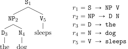
6.2 An Example
In the remainder of this section we give an example that illustrates how the algorithm in Figure 4 is correct, and gives the basic intuition behind the proof in Section A.1. While we concentrate on the algorithm in Figure 4, the intuition behind the algorithm in Figure 5 is very similar.
S1 NP2 D3 the
N4 dog
V5 sleeps
r1“ S Ñ NP V r2“ NP Ñ D N r3“ D Ñ the r4“ N Ñ dog r5“ V Ñ sleeps
Figure 6: An s-tree, and its sequence of rules. (For convenience we have numbered the nodes in the tree.)
1. We first show that the algorithm in Figure 4, when run on the tree in Figure 6, calculates the probability of the tree as
CSÑN P V
pCN PÑD N pc8
DÑthe, c8NÑdogq, c8VÑsleepsqc1S. Note that this expression mirrors the structure of the tree, with c8
aÑx terms for the leaves, CaÑb c terms for each rule production aÑb c in the tree, and a c1
S term for the root.
2. We then show that under the assumptions in the theorem, the following identity holds:
CSÑN P V
pCN PÑD N pc8
DÑthe, c8NÑdogq, c8VÑsleepsqc1S.
“ TSÑN P VpTN PÑD NpqDÑthe, qNÑdogq, qVÑsleepsqπS (3)
This follows because the Ga and pGaq´1 terms for the various non-terminals in the tree cancel. Note that the expression in Eq. 3 again follows the structure of the tree, but withqaÑx terms for the leaves, TaÑb c terms for each rule productionaÑb cin the tree, and aπS term for the root.
3. Finally, we show that the expression in Eq. 3 implements the conventional dynamic-programming method for calculation of the tree probability, as described in Eqs. 11–13 below.
We now go over these three points in detail. The algorithm in Figure 4 calculates the following terms (each fi is anm-dimensional row vector):
f3 “ c8 DÑthe f4 “ c8NÑdog f5 “ c8VÑsleeps f2 “ CN PÑD N
pf3, f4q
f1 “ CSÑN P V
The final quantity returned by the algorithm is
f1c1S“
ÿ
h
fh1rc1Ssh.
Combining the definitions above, it can be seen that
f1c1S “CSÑN P VpCN PÑD NpcD8Ñthe, c8NÑdogq, c8VÑsleepsqc1S, demonstrating that point 1 above holds.
Next, given the assumptions in the theorem, we show point 2, that is, that
CSÑN P VpCN PÑD Npc8DÑthe, c8NÑdogq, c8VÑsleepsqc1S
“ TSÑN P VpTN PÑD NpqDÑthe, qNÑdogq, qVÑsleepsqπS. (4)
This follows because the Ga and pGaq´1 terms in the theorem cancel. More specifically, we have
f3 “ c8DÑthe“qDÑthepGDq´1 (5) f4 “ c8NÑdog “qNÑdogpGNq´1 (6)
f5 “ c8VÑsleeps“qVÑsleepspGVq´1 (7)
f2 “ CN PÑD N
pf3, f4q “TN PÑD N
pqDÑthe, qDÑdogqpGN Pq´1 (8) f1 “ CSÑN P V
pf2, f5q “TSÑN P V
pTN PÑD N
pqDÑthe, qNÑdogq, qVÑsleepsqpGSq´1(9)
Eqs. 5, 6, 7 follow by the assumptions in the theorem. Eq. 8 follows because by the assump-tions in the theorem
CN PÑD N
pf3, f4q “ TN PÑD N
pf3GD, f4GNqpGN Pq´1
hence
CN PÑD Npf3, f4q “ TN PÑD NpqDÑthepGDq´1GD, qNÑdogpGNq´1GNqpGN Pq´1 “ TN PÑD NpqDÑthe, qNÑdogqpGN Pq´1
Eq. 9 follows in a similar manner.
It follows by the assumption that c1S “GSπS that CSÑN P V
pCN PÑD N pc8
DÑthe, c8NÑdogq, c8VÑsleepsqc1S
“ TSÑN P VpTN PÑD NpqDÑthe, qNÑdogq, qVÑsleepsqpGSq´1GSπS “ TSÑN P V
pTN PÑD N
pqDÑthe, qNÑdogq, qVÑsleepsqπS (10)
The final step (point 3) is to show that the expression in Eq. 10 correctly calculates the probability of the example tree. First consider the term TN PÑD N
is anm-dimensional row vector, call thisb2. By the definition of the tensor TN PÑD N, we have
b2h “ “TN PÑD NpqDÑthe, qNÑdogq
‰
h
“ ÿ
h2,h3
tpN P ÑD N, h2, h3|h, N Pq ˆqpDÑthe|h2, Dq ˆqpN Ñdog|h3, Nq(11)
By a similar calculation,TSÑN P V
pTN PÑD N
pqDÑthe, qNÑdogq, qVÑsleepsq—call this vector b1—is
b1h “
ÿ
h2,h3
tpSÑN P V, h2, h3|h, Sq ˆb2h2 ˆqpV Ñsleeps|h3, Vq (12) Finally, the probability of the full tree is calculated as
ÿ
h
b1hπSh. (13) It can be seen that the expression in Eq. 4 implements the calculations in Eqs. 11, 12 and 13, which are precisely the calculations used in the conventional dynamic programming algorithm for calculation of the probability of the tree.
7. Estimating the Tensor Model
A crucial result is that it is possible to directly estimate parameters CaÑb c, c8
aÑx and c1a that satisfy the conditions in Theorem 3, from a training sample consisting of s-trees (i.e., trees where hidden variables are unobserved). We first describe random variables underlying the approach, then describe observable representations based on these random variables.
7.1 Random Variables Underlying the Approach
Each s-tree with N rules r1. . . rN has N nodes. We will use the s-tree in Figure 1 as a running example.
Each node has an associated rule: for example, node 2 in the tree in Figure 1 has the rule NP Ñ D N. If the rule at a node is of the form aÑb c, then there are left and right inside treesbelow the left child and right child of the rule. For example, for node 2 we have a left inside tree rooted at node 3, and a right inside tree rooted at node 4 (in this case the left and right inside trees both contain only a single rule production, of the form a Ñ x; however in the general case they might be arbitrary subtrees).
In addition, each node has an outside tree. For node 2, the outside tree is S
NP VP
V
saw P
him
The outside tree contains everything in the s-tree r1. . . rN, excluding the subtree below node i.
• Sample a full treer1. . . rN, h1. . . hN from the PMFppr1. . . rN, h1. . . hNq. • Choose a nodeiuniformly at random fromrNs.
If the ruleri for the nodeiis of the formaÑb c, we define random variables as follows:
• R1 is equal to the ruleri (e.g., NPÑD N).
• T1 is the inside tree rooted at node i. T2 is the inside tree rooted at the left child of nodei, and T3 is the inside tree rooted at the right child of node i.
• H1, H2, H3 are the hidden variables associated with node i, the left child of node i, and the right child of nodeirespectively.
• A1, A2, A3 are the labels for nodei, the left child of nodei, and the right child of node irespectively. (e.g.,A1 “NP,A2“D,A3“N.)
• O is the outside tree at node i.
• B is equal to 1 if nodei is at the root of the tree (i.e.,i“1), 0 otherwise.
If the rule ri for the selected node i is of the form a Ñ x, we have random variables R1, T1, H1,
A1, O, B as defined above, butH2, H3, T2, T3, A2, and A3 are not defined.
We assume a function ψ that maps outside trees o to feature vectors ψpoq P Rd 1
. For example, the feature vector might track the rule directly above the node in question, the word following the node in question, and so on. We also assume a function φ that maps inside trees t to feature vectors φptq P Rd. As one example, the function φ might be an
indicator function tracking the rule production at the root of the inside tree. Later we give formal criteria for what makes good definitions of ψpoq and φptq. One requirement is that d1
ěmand děm.
In tandem with these definitions, we assume projection matrices Ua P Rpdˆmq and
Va P Rpd 1ˆmq
for all a P N. We then define additional random variables Y1, Y2, Y3, Z as
Y1 “ pUa1qJφpT1q Z “ pVa1qJψpOq Y2 “ pUa2qJφpT2q Y3 “ pUa3qJφpT3q
whereai is the value of the random variable Ai. Note that Y1, Y2, Y3, Z are all inRm.
7.2 Observable Representations
Given the definitions in the previous section, our representation is based on the following matrix, tensor and vector quantities, defined for allaPN, for all rules of the formaÑb c, and for all rules of the formaÑx respectively:
Σa “ ErY1ZJ|A1“as, DaÑb c
“ E“vR1 “aÑb cwZY2JY3J|A1 “a ‰
Assuming access to functionsφandψ, and projection matricesUa andVa, these quantities can be estimated directly from training data consisting of a set of s-trees (see Section 8).
Our observable representation then consists of:
CaÑb c
py1, y2q “ DaÑb c
py1, y2qpΣaq´1, (14) c8
aÑx “ d8aÑxpΣaq´1, (15)
c1a “ ErvA1“awY1|B “1s. (16) We next introduce conditions under which these quantities satisfy the conditions in Theo-rem 3.
The following definition will be important:
Definition 5 For all aPN, we define the matricesIaPRpdˆmq and JaPRpd 1ˆmq
as
rIasi,h “ErφipT1q |H1 “h, A1 “as,
rJasi,h“ErψipOq |H1 “h, A1 “as.
In addition, for any aPN, we useγaPRm to denote the vector with γah“PpH1 “h|A1“
aq.
The correctness of the representation will rely on the following conditions being satisfied (these are parallel to conditions 1 and 2 in Hsu et al. (2009)):
Condition 1 @a P N, the matrices Ia and Ja are of full rank (i.e., they have rank m). For all aPN, for all hP rms, γa
h ą0.
Condition 2 @a P N, the matrices Ua P Rpdˆmq and Va P Rpd 1ˆmq
are such that the matrices Ga“ pUaqJIa and Ka“ pVaqJJa are invertible.
We can now state the following theorem:
Theorem 6 Assume conditions 1 and 2 are satisfied. For all aPN, define Ga “ pUaqJIa. Then under the definitions in Eqs. 14-16:
1. For all rules aÑb c,CaÑb c
py1, y2q “`TaÑb c
py1Gb, y2Gcq˘pGaq´1 2. For all rules aÑx, c8
aÑx“qaÑxpGaq´1. 3. For all aPN, c1a“Gaπa
Proof: The following identities hold (see Section A.2):
DaÑb cpy1, y2q “
´
TaÑb cpy1Gb, y2Gcq
¯
diagpγaqpKaqJ (17) d8
aÑx “ qaÑxdiagpγaqpKaqJ (18) Σa “ GadiagpγaqpKaqJ (19)
Under conditions 1 and 2, Σa is invertible, and pΣaq´1 “ ppKaqJq´1pdiagpγaqq´1pGaq´1. The identities in the theorem follow immediately.
This theorem leads directly to the spectral learning algorithm, which we describe in the next section. We give a sketch of the approach here. Assume that we have a training set consisting of skeletal trees (no latent variables are observed) generated from some under-lying L-PCFG. Assume in addition that we have definitions ofφ,ψ,Ua and Va such that conditions 1 and 2 are satisfied for the L-PCFG. Then it is straightforward to use the train-ing examples to derive i.i.d. samples from the joint distribution over the random variables
pA1, R1, Y1, Y2, Y3, Z, Bq used in the definitions in Eqs. 14–16. These samples can be used to estimate the quantities in Eqs. 14–16; the estimated quantities ˆCaÑb c, ˆc8
aÑx and ˆc1a can then be used as inputs to the algorithms in Figures 4 and 5. By standard arguments, the estimates ˆCaÑb c, ˆc8
aÑx and ˆc1a will converge to the values in Eqs. 14–16.
The following lemma justifies the use of an SVD calculation as one method for finding values for Ua andVa that satisfy condition 2, assuming that condition 1 holds:
Lemma 7 Assume that condition 1 holds, and for all aPN define
Ωa“ErφpT1q pψpOqqJ|A1“as (21) Then ifUais a matrix of themleft singular vectors ofΩacorresponding to non-zero singular values, and Va is a matrix of the m right singular vectors of Ωa corresponding to non-zero singular values, then condition 2 is satisfied.
Proof sketch: It can be shown that Ωa“IadiagpγaqpJaqJ. The remainder is similar to
the proof of lemma 2 in Hsu et al. (2009).
The matrices Ωa can be estimated directly from a training set consisting of s-trees, assuming that we have access to the functionsφand ψ. Similar arguments to those of Hsu et al. (2009) can be used to show that with a sufficient number of samples, the resulting estimates of Ua andVasatisfy condition 2 with high probability.
8. Deriving Empirical Estimates
Figure 7 shows an algorithm that derives estimates of the quantities in Eqs. 14, 15, and 16. As input, the algorithm takes a sequence of tuples prpi,1q, tpi,1q, tpi,2q, tpi,3q, opiq, bpiq
q for iP rMs.
These tuples can be derived from a training set consisting of s-treesτ1. . . τM as follows: ‚ @iP rMs, choose a single node ji uniformly at random from the nodes in τi. Define rpi,1qto be the rule at nodej
i. tpi,1qis the inside tree rooted at nodeji. Ifrpi,1qis of the form aÑb c, thentpi,2q is the inside tree under the left child of node j
i, and tpi,3q is the inside tree under the right child of nodeji. Ifrpi,1q is of the formaÑx, thentpi,2q“tpi,3q“NULL. opiq is the outside tree at node j
i. bpiq is 1 if nodeji is at the root of the tree, 0 otherwise. Under this process, assuming that the s-treesτ1. . . τM are i.i.d. draws from the distribu-tionppτqover s-trees under an L-PCFG, the tuplesprpi,1q, tpi,1q, tpi,2q, tpi,3q, opiq, bpiqq are i.i.d. draws from the joint distribution over the random variables R1, T1, T2, T3, O, B defined in the previous section.
The matrices are then used to project inside and outside treestpi,1q, tpi,2q, tpi,3q, opiq down to m-dimensional vectors ypi,1q, ypi,2q, ypi,3q, zpiq; these vectors are used to derive the estimates of CaÑb c,c8
aÑx, andc1a. For example, the quantities DaÑb c
“ E“vR1“aÑb cwZY2JY3J|A1“a ‰
d8aÑx “ E“vR1“aÑxwZJ|A1 “a‰ can be estimated as
ˆ
DaÑb c “δaˆ M
ÿ
i“1
vrpi,1q “aÑb cwzpiqpypi,2qqJpypi,3qqJ
ˆ
d8aÑx“δaˆ M
ÿ
i“1
vrpi,1q “aÑxwpzpiqqJ
whereδa“1{
řM
i“1vai “aw, and we can then set ˆ
CaÑb c
py1, y2q “DˆaÑb c
py1, y2qpΣˆaq´1
ˆ c8
aÑx“dˆ8aÑxpΣˆaq´1.
We now state a PAC-style theorem for the learning algorithm. First, we give the fol-lowing assumptions and definitions:
• We have an L-PCFGpN,I,P, m, n, t, q, πq. The samples used in Figures 7 and 8 are i.i.d. samples from the L-PCFG (for simplicity of analysis we assume that the two algorithms use independent sets of M samples each: see above for how to draw i.i.d. samples from the L-PCFG).
• We have functions φptq PRd andψpoq PRd 1
that map inside and outside trees respec-tively to feature vectors. We will assume without loss of generality that for all inside trees||φptq||2ď1, and for all outside trees||ψpoq||2 ď1.
• See Section 7.2 for a definition of the random variables
pR1, T1, T2, T3, A1, A2, A3, H1, H2, H3, O, Bq, and the joint distribution over them.
• For allaPN define
Ωa“ErφpT1qpψpOqqJ|A1 “as
and defineIa PRdˆm to be the matrix with entries
rIasi,h “ErφipT1q|A1 “a, H1“hs • Define
σ“min a σmpΩ
a q
and
ξ“min a σmpI
a q
• Define
γ “ min a,b,cPN,h1,h2,h3Prms
tpaÑb c, h2, h3|a, h1q
• DefineTpa, Nq to be the set of of all skeletal trees withN binary rules (hence 2N`1 rules in total), with non-terminal aat the root of the tree.
The following theorem gives a bound on the sample complexity of the algorithm:
Theorem 8 There exist constants C1, C2, C3, C4, C5 such that the following holds. Pick any ą 0, any value for δ such that 0 ă δ ă 1, and any integer N such that N ě 1. Define L “ log2|Nδ|`1. Assume that the parameters CˆaÑb c, ˆc8
aÑx and ˆc1a are output from the algorithm in Figure 7, with values for Na,Ma andR such that
@aPI, Naě
C1LN2m2
γ22ξ4σ4 @aPP, Naě
C2LN2m2n 2σ4
@aPI, Maě
C3LN2m2
γ22ξ4σ2 @aPP, Maě
C4LN2m2 2σ2 Rě C5LN
2m3 2σ2
It follows that with probability at least 1´δ, for allaPN,
ÿ
tPTpa,Nq
|pˆptq ´pptq| ď
, wherepˆptq is the output from the algorithm in Figure 4 with parametersCˆaÑb c,cˆ8 aÑx and ˆ
c1a, andpptq is the probability of the skeletal tree under the L-PCFG. See Appendix B for a proof.
The method described of selecting a single tupleprpi,1q, tpi,1q, tpi,2q, tpi,3q, opiq, bpiq
qfor each s-tree ensures that the samples are i.i.d., and simplifies the analysis underlying Theorem 8. In practice, an implementation should use all nodes in all trees in training data; by Rao-Blackwellization we know such an algorithm would be better than the one presented, but the analysis of how much better would be challenging (Bickel and Doksum, 2006; section 3.4.2). It would almost certainly lead to a faster rate of convergence of ˆptop.
9. Discussion
There are several applications of the method. The most obvious is parsing with L-PCFGs (Cohen et al., 2013).3 The approach should be applicable in other cases where EM has traditionally been used, for example in semi-supervised learning. Latent-variable HMMs for sequence labeling can be derived as special case of our approach, by converting tagged sequences to right-branching skeletal trees (Stratos et al., 2013).
3. Parameters can be estimated using the algorithm in Figure 7; for a test sentencex1. . . xN we can first use the algorithm in Figure 5 to calculate marginalsµpa, i, jq, then use the algorithm of Goodman (1996) to find arg maxτPTpxq
ř
Inputs: Training examplesprpi,1q, tpi,1q, tpi,2q, tpi,3q, opiq, bpiq
q foriP t1. . . Mu, whererpi,1q is a context free rule; tpi,1q, tpi,2q and tpi,3q are inside trees; opiq is an outside tree; and bpiq“1 if the rule is at the root of tree, 0 otherwise. A functionφthat maps inside trees tto feature-vectors φptq PRd. A functionψ that maps outside trees oto feature-vectors
ψpoq PRd 1
.
Definitions: For each a P N, define Na “
řM
i“1vai “aw. Define R “ řM
i“1vbpiq “ 1w. (These definitions will be used in Theorem 8.)
Algorithm:
Define ai to be the non-terminal on the left-hand side of rule rpi,1q. If rpi,1q is of the formaÑb c, definebi to be the non-terminal for the left-child of rpi,1q, andci to be the non-terminal for the right-child.
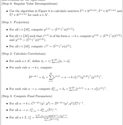
(Step 0: Singular Value Decompositions)
• Use the algorithm in Figure 8 to calculate matrices ˆUaPRpdˆmq, ˆVaPRpd 1ˆmq
and ˆ
ΣaPRpmˆmq for each aPN.
(Step 1: Projection)
• For alliP rMs, computeypi,1q
“ pUˆaiqJφptpi,1qq.
• For alliP rMssuch thatrpi,1qis of the formaÑb c, computeypi,2q“ pUˆbiqJφptpi,2qq
andypi,3q
“ pUˆciqJφptpi,3qq.
• For alliP rMs, computezpiq“ pVˆaiqJψpopiqq.
(Step 2: Calculate Correlations)
• For eachaPN, defineδa“1{
řM
i“1vai “aw. • For each rule aÑb c, compute
ˆ DaÑb c
“δaˆ M
ÿ
i“1
vrpi,1q
“aÑb cwzpiq
pypi,2q
qJpypi,3q
qJ.
• For each rule aÑx, compute ˆd8
aÑx “δaˆ
řM
i“1vrpi,1q “aÑxwpzpiqqJ. (Step 3: Compute Final Parameters)
• For allaÑb c, ˆCaÑb c
py1, y2q “DˆaÑb c
py1, y2qpΣˆaq´1. • For allaÑx, ˆc8
aÑx“dˆ8aÑxpΣˆaq´1. • For allaPI, ˆc1a“
řM
i“1vai“aandbpiq“1wypi,1q
řM
i“1vbpiq“1w
.
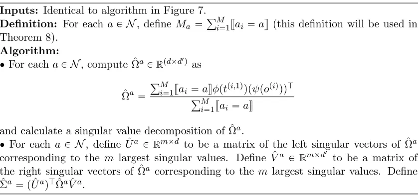
Inputs: Identical to algorithm in Figure 7. Definition: For each aPN, define Ma “
řM
i“1vai “aw (this definition will be used in Theorem 8).
Algorithm:
‚For each aPN, compute ˆΩaPRpdˆd 1q
as
ˆ Ωa“
řM
i“1vai“awφptpi,1qqpψpopiqqqJ
řM
i“1vai “aw and calculate a singular value decomposition of ˆΩa.
‚ For each a P N, define ˆUa P Rmˆd to be a matrix of the left singular vectors of ˆΩa
corresponding to the m largest singular values. Define ˆVa P Rmˆd 1
to be a matrix of the right singular vectors of ˆΩa corresponding to the m largest singular values. Define
ˆ
Σa“ pUˆaqJΩˆaVˆa.
Figure 8: Singular value decompositions.
In terms of efficiency, the first step of the algorithm in Figure 7 requires an SVD cal-culation: modern methods for calculating SVDs are very efficient (e.g., see Dhillon et al., 2011 and Tropp et al., 2009). The remaining steps of the algorithm require manipulation of tensors or vectors, and requireOpM m3q time.
The sample complexity of the method depends on the minimum singular values of Ωa; these singular values are a measure of how well correlatedψ andφare with the unobserved hidden variable H1. Experimental work is required to find a good choice of values for ψ and φfor parsing.
For simplicity we have considered the case where each non-terminal has the same num-ber,m, of possible hidden values. It is simple to generalize the algorithms to the case where the number of hidden values varies depending on the non-terminal; this is important in applications such as parsing.
Acknowledgements
Appendix A. Proofs of Theorems 1 and 2
This section gives proofs of Theorems 3 and 6.
A.1 Proof of Theorem 3
The key idea behind the proof of Theorem 3 is to show that the algorithms in Figures 4 and 5 compute the same quantities as the conventional version of the inside outside algorithms, as shown in Figures 2 and 3.
First, the following lemma leads directly to the correctness of the algorithm in Figure 4:
Lemma 9 Assume that conditions 1-3 of Theorem 3 are satisfied, and that the input to the algorithm in Figure 4 is an s-tree r1. . . rN. Define ai for iP rNs to be the non-terminal on the left-hand-side of rule ri. For all i P rNs, define the row vector bi P Rp1ˆmq to be
the vector computed by the conventional inside-outside algorithm, as shown in Figure 2, on the s-tree r1. . . rN. Define fi P Rp1ˆmq to be the vector computed by the tensor-based
inside-outside algorithm, as shown in Figure 4, on the s-tree r1. . . rN. Then for all iP rNs, fi“bipGpaiqq´1. It follows immediately that
f1c1a1 “b1pGpa1qq´1Ga1π a1 “b
1π a1 “
ÿ
h
b1hπpa, hq.
Hence the output from the algorithms in Figures 2 and 4 is the same, and it follows that the tensor-based algorithm in Figure 4 is correct.
This lemma shows a direct link between the vectorsfi calculated in the algorithm, and the termsbih, which are terms calculated by the conventional inside algorithm: eachfi is a linear transformation (throughGai) of the corresponding vector bi.
Proof: The proof is by induction.
First consider the base case. For any leaf—i.e., for any i such that ai P P—we have bih “qpri|h, aiq, and it is easily verified thatfi “bipGpaiqq´1.
The inductive case is as follows. For all i P rNssuch that ai PI, by the definition in the algorithm,
fi “ Cri
pfβ, fγq “
´ Tri
pfβGaβ, fγGaγ
q
¯
pGai
q´1
Assuming by induction thatfβ “bβpGpaβqq´1 andfγ “bγpGpaγqq´1, this simplifies to
fi“
´ Tri
pbβ, bγq
¯
pGai
q´1. (22)
By the definition of the tensor Tri,
”
Tripbβ, bγq
ı
h “
ÿ
h2Prms,h3Prms
tpri, h2, h3|ai, hqbβh2bγh3
But by definition (see the algorithm in Figure 2),
bih“ ÿ h2Prms,h3Prms
hencebi “Tripbβ, bγqand the inductive case follows immediately from Eq. 22.
Next, we give a similar lemma, which implies the correctness of the algorithm in Figure 5:
Lemma 10 Assume that conditions 1-3 of Theorem 3 are satisfied, and that the input to the algorithm in Figure 5 is a sentence x1. . . xN. For any aPN, for any 1ďiďj ďN, define α¯a,i,j P Rp1ˆmq, β¯a,i,j P Rpmˆ1q and µ¯pa, i, jq P R to be the quantities computed
by the conventional inside-outside algorithm in Figure 3 on the input x1. . . xN. Define αa,i,j P Rp1ˆmq, βa,i,j P Rpmˆ1q and µpa, i, jq P R to be the quantities computed by the
algorithm in Figure 3.
Then for all iP rNs, αa,i,j “ α¯a,i,jpGaq´1 and βa,i,j “Gaβ¯a,i,j. It follows that for all pa, i, jq,
µpa, i, jq “αa,i,jβa,i,j “α¯a,i,jpGaq´1Gaβ¯a,i,j “α¯a,i,jβ¯a,i,j “µ¯pa, i, jq.
Hence the outputs from the algorithms in Figures 3 and 5 are the same, and it follows that the tensor-based algorithm in Figure 5 is correct.
Thus the vectorsαa,i,j andβa,i,j are linearly related to the vectors ¯αa,i,j and ¯βa,i,j, which are the inside and outside terms calculated by the conventional form of the inside-outside algorithm.
Proof: The proof is by induction, and is similar to the proof of Lemma 9. First, we prove that the inside terms satisfy the relation αa,i,j “α¯a,i,jpGaq´1.
The base case of the induction is as follows. By definition, for anyaPP, iP rNs, hP rms, we have ¯αha,i,i “ qpa Ñ xi|h, aq. We also have for any a P P, i P rNs, αa,i,i “ c8aÑxi “
qaÑxipG
aq´1. It follows directly that αa,i,i “α¯a,i,ipGaq´1 for any aPP, iP rNs.
The inductive case is as follows. By definition, we have @aPI,1ďiăj ďN, hP rms
¯ αa,i,jh “
j´1 ÿ
k“i
ÿ
b,c
ÿ
h2Prms ÿ
h3Prms
tpaÑb c, h2, h3|h, aq ˆα¯b,i,kh 2 ˆα¯
c,k`1,j h3 .
We also have @aPI,1ďiăjďN,
αa,i,j “ j´1
ÿ
k“i
ÿ
b,c
CaÑb cpαb,i,k, αc,k`1,jq (23)
“ j´1
ÿ
k“i
ÿ
b,c
´
TaÑb cpαb,i,kGb, αc,k`1,jGcq
¯
pGaq´1 (24)
“ j´1
ÿ
k“i
ÿ
b,c
´ TaÑb c
pα¯b,i,k,α¯c,k`1,j ¯
pGaq´1 (25)
“ α¯a,i,jpGaq´1. (26)
Eq. 23 follows by the definitions in algorithm 5. Eq. 24 follows by the assumption in the theorem that
CaÑb cpy1, y2q “
´
TaÑb cpy1Gb, y2Gcq
¯
Eq. 25 follows because by the inductive hypothesis,
αb,i,k “α¯b,i,kpGbq´1
and
αc,k`1,j “α¯c,k`1,jpGcq´1. Eq. 26 follows because
” TaÑb c
pα¯b,i,k,α¯c,k`1,jq
ı
h “
ÿ
h2,h3
tpaÑb c, h2, h3|h, aqα¯b,i,kh2 α¯c,kh3`1,j
hence
j´1 ÿ
k“i
ÿ
b,c TaÑb c
pα¯b,i,k,α¯c,k`1,jq “α¯a,i,j.
We now turn the outside terms, proving that βa,i,j “ Gaβ¯a,i,j. The proof is again by induction.
The base case is as follows. By the definitions in the algorithms, for all aPI, βa,1,n “ c1a“Gaπa, and for all aPI, hP rms, ¯βa,h1,n “πpa, hq. It follows directly that for all aPI,
βa,1,n“Gaβ¯a,1,n.
The inductive case is as follows. By the definitions in the algorithms, we have @a P
N,1ďiďjďN, hP rms
¯
βha,i,j “γh1,a,i,j`γh2,a,i,j where
γh1,a,i,j “ i´1 ÿ
k“1 ÿ
bÑc a
ÿ
h2Prms ÿ
h3Prms
tpbÑc a, h3, h|h2, bq ˆβ¯hb,k,j2 ˆα¯c,k,ih3 ´1
γh2,a,i,j “ N
ÿ
k“j`1 ÿ
bÑa c
ÿ
h2Prms ÿ
h3Prms
tpbÑa c, h, h3|h2, bq ˆβ¯hb,i,k 2 ˆα¯
c,j`1,k h3
and @aPN,1ďiďjďN,
βa,i,j “ i´1 ÿ
k“1 ÿ
bÑc a
Cp1bÑ,2qc apβb,k,j, αc,k,i´1q ` N
ÿ
k“j`1 ÿ
bÑa c
Cp1bÑ,3qa cpβb,i,k, αc,j`1,kq.
Critical identities are
i´1 ÿ
k“1 ÿ
bÑc a CbÑc a
p1,2q pβ
b,k,j, αc,k,i´1
q “ Gaγ1,a,i,j (27)
N
ÿ
k“j`1 ÿ
bÑa c CbÑa c
p1,3q pβb,i,k, αc,j`1,kq “ Gaγ2,a,i,j (28) from which βa,i,j “Gaβ¯a,i,j follows immediately.
• By the inductive hypothesis, βb,k,j “Gbβ¯b,k,j and βb,i,k “Gbβ¯b,i,k.
• By correctness of the inside terms, as shown earlier in this proof, it holds that αc,k,i´1 “α¯c,k,i´1pGcq´1 andαc,j`1,k “α¯c,j`1,kpGcq´1.
• By the assumptions in the theorem,
CaÑb c
py1, y2q “
´ TaÑb c
py1Gb, y2Gcq
¯
pGaq´1.
It follows (see Lemma 11) that
CbÑc a
p1,2q pβb,k,j, αc,k,i´1q “ Ga ´
TbÑc a
p1,2q ppGbq´1βb,k,j, αc,k,i´1Gcq ¯
“ Ga ´
Tp1bÑ,2qc apβ¯b,k,j,α¯c,k,i´1q
¯
and
Cp1bÑ,3qa cpβb,i,k, αc,j`1,kq “ Ga ´
Tp1bÑ,3qa cpβ¯b,i,k,α¯c,j`1,kq
¯
Finally, we give the following Lemma, as used above:
Lemma 11 Assume we have tensors C P Rmˆmˆm and T P Rmˆmˆm such that for any
y2, y3,
Cpy2, y3q “`Tpy2A, y3Bq˘D where A, B, D are matrices in Rmˆm. Then for anyy1, y2,
Cp1,2qpy1, y2q “B `
Tp1,2qpDy1, y2Aq ˘
(29)
and for any y1, y3,
Cp1,3qpy1, y3q “A `
Tp1,3qpDy1, y3Bq ˘
. (30)
Proof: Consider first Eq. 29. We will prove the following statement:
@y1, y2, y3, y3Cp1,2qpy1, y2q “y3B `
Tp1,2qpDy1, y2Aq ˘
This statement is equivalent to Eq. 29.
First, for all y1, y2, y3, by the assumption that Cpy2, y3q “`Tpy2A, y3Bq˘D, Cpy2, y3qy1“Tpy2A, y3BqDy1
hence
ÿ
i,j,k
Ci,j,ky1iy2jyk3“
ÿ
i,j,k
Ti,j,kzi1z2jzk3 (31)
In addition, it is easily verified that
y3Cp1,2qpy1, y2q “ ÿ
i,j,k
Ci,j,kyi1y2jy3k (32) y3B`Tp1,2qpDy1, y2Aq˘ “ ÿ
i,j,k
Ti,j,kz1izj2zk3 (33)
where again z1 “Dy1,z2 “y2A,z3 “y3B. Combining Eqs. 31, 32, and 33 gives y3Cp1,2qpy1, y2q “y3B`Tp1,2qpDy1, y2Aq˘,
thus proving the identity in Eq. 29.
The proof of the identity in Eq. 30 is similar, and is omitted for brevity.
A.2 Proof of the Identity in Eq. 17
We now prove the identity in Eq. 17, repeated here:
DaÑb cpy1, y2q “
´
TaÑb cpy1Gb, y2Gcq
¯
diagpγaqpKaqJ.
Recall that
DaÑb c “E“vR1 “aÑb cwZY2JY3J|A1 “a‰, or equivalently
DaÑb c
i,j,k “ErvR1“aÑb cwZiY2,jY3,k|A1 “as. Using the chain rule, and marginalizing over hidden variables, we have
Dai,j,kÑb c “ ErvR1 “aÑb cwZiY2,jY3,k|A1 “as
“ ÿ
h1,h2,h3Prms
ppaÑb c, h1, h2, h3|aqErZiY2,jY3,k|R1“aÑb c, h1, h2, h3s.
By definition, we have
ppaÑb c, h1, h2, h3|aq “γha1 ˆtpaÑb c, h2, h3|h1, aq
In addition, under the independence assumptions in the L-PCFG, and using the definitions of Ka andGa, we have
ErZiY2,jY3,k|R1 “aÑb c, h1, h2, h3s
“ ErZi|A1 “a, H1“h1s ˆErY2,j|A2 “b, H2 “h2s ˆErY3,k|A3“c, H3 “h3s “ Ki,ha 1 ˆGbj,h2 ˆGck,h3.
Putting this all together gives
Dai,j,kÑb c “ ÿ h1,h2,h3Prms
γha1ˆtpaÑb c, h2, h3|h1, aq ˆKi,ha 1ˆGbj,h2 ˆGck,h3
“ ÿ
h1Prms
γha1ˆKi,ha 1ˆ ÿ h2,h3Prms
By the definition of tensors,
rDaÑb cpy1, y2qsi
“ ÿ
j,k
DaÑb c i,j,k yj1yk2
“
ÿ
h1Prms
γha1ˆKi,ha 1ˆ
ÿ
h2,h3Prms
tpaÑb c, h2, h3|h1, aq ˆ ˜
ÿ
j
yj1Gbj,h2 ¸
ˆ
˜ ÿ
k
y2kGck,h3 ¸
“ ÿ
h1Prms
γha1ˆKi,ha 1ˆ
” TaÑb c
py1Gb, y2Gcq
ı
h1
. (34)
The last line follows because by the definition of tensors,
”
TaÑb cpy1Gb, y2Gcq
ı
h1
“ ÿ
h2,h3
Tha1Ñ,hb c2,h3 ”
y1Gb ı
h2 “
y2Gc‰h 3
and we have
TaÑb c
h1,h2,h3 “ tpaÑb c, h2, h3|h1, aq ”
y1Gb ı
h2
“ ÿ
j
y1jGbj,h2 “
y2Gc‰h 3 “
ÿ
k
y2kGck,h3.
Finally, the required identity
DaÑb c
py1, y2q “
´ TaÑb c
py1Gb, y2Gcq
¯
diagpγaqpKaqJ
follows immediately from Eq. 34.
A.3 Proof of the Identity in Eq. 18
We now prove the identity in Eq. 18, repeated below:
d8
aÑx“qaÑxdiagpγaqpKaqJ. Recall that by definition
d8 aÑx“E
“
vR1 “aÑxwZJ|A1“a ‰
,
or equivalently
rd8aÑxsi“ErvR1“aÑxwZi|A1 “as. Marginalizing over hidden variables, we have
rd8aÑxsi “ ErvR1 “aÑxwZi|A1“as “
ÿ
h
By definition, we have
ppaÑx, h|aq “γhaqpaÑx|h, aq “γharqaÑxsh.
In addition, by the independence assumptions in the L-PCFG, and the definition ofKa,
ErZi|H1 “h, R1 “aÑxs “ErZi|H1“h, A1“as “Ki,ha . Putting this all together gives
rd8aÑxsi“
ÿ
h
γharqaÑxshKi,ha
from which the required identity
d8
aÑx “qaÑxdiagpγaqpKaqJ
follows immediately.
A.4 Proof of the Identity in Eq. 19
We now prove the identity in Eq. 19, repeated below:
Σa “GadiagpγaqpKaqJ
Recall that by definition
Σa“ErY1ZJ|A1 “as or equivalently
rΣasi,j “ErY1,iZj|A1 “as Marginalizing over hidden variables, we have
rΣasi,j “ ErY1,iZj|A1 “as
“ ÿ
h
pph|aqErY1,iZj|H1“h, A1“as
By definition, we have
γha“pph|aq
In addition, under the independence assumptions in the L-PCFG, and using the definitions of Ka andGa, we have
ErY1,iZj|H1 “h, A1 “as “ ErY1,i|H1 “h, A1 “as ˆErZj|H1 “h, A1 “as
“ Gai,hKj,ha Putting all this together gives
rΣasi,j “ÿ h
γhaGai,hKj,ha
from which the required identity
Σa “GadiagpγaqpKaqJ
A.5 Proof of the Identity in Eq. 20
We now prove the identity in Eq. 19, repeated below:
c1a“Gaπa. Recall that by definition
c1a“ErvA1 “awY1|B “1s, or equivalently
rc1asi“ErvA1“awY1,i|B “1s. Marginalizing over hidden variables, we have
rc1asi “ ErvA1 “awY1,i|B “1s “
ÿ
h
PpA1 “a, H1“h|B“1qErY1,i|A1 “a, H1“h, B“1s.
By definition we have
PpA1 “a, H1“h|B“1q “πpa, hq
By the independence assumptions in the PCFG, and the definition of Ga, we have
ErY1,i|A1“a, H1 “h, B“1s “ ErY1,i|A1 “a, H1“hs
“ Gai,h.
Putting this together gives
rc1asi“
ÿ
h
πpa, hqGai,h
from which the required identity
c1a“Gaπa
follows.
Appendix B. Proof of Theorem 8
In this section we give a proof of Theorem 8. The proof relies on three lemmas:
• In Section B.1 we give a lemma showing that if estimates ˆCaÑb c, ˆc
aÑx and ˆc1a are close (up to linear transforms) to the parameters of an L-PCFG, then the distribution defined by the parameters is close (inl1-norm) to the distribution under the L-PCFG. • In Section B.2 we give a lemma showing that if the estimates ˆΩa, ˆDaÑb c, ˆd8
aÑx and ˆ
c1a are close to the underlying values being estimated, the estimates ˆCaÑb c, ˆc
aÑx and ˆ
c1
a are close (up to linear transforms) to the parameters of the underlying L-PCFG.
• In Section B.3 we give a lemma relating the number of samples in the estimation algorithm to the errors in estimating ˆΩa, ˆDaÑb c, ˆd8
B.1 A Bound on How Errors Propagate
In this section we show that if estimated tensors and vectors ˆCaÑb c, ˆc8
aÑx and ˆc1a are sufficiently close to the underlying parameters TaÑb c, q8
aÑx, and πa of an L-PCFG, then the distribution under the estimated parameters will be close to the distribution under the L-PCFG. Section B.1.1 gives assumptions and definitions; Lemma 12 then gives the main lemma; the remainder of the section gives proofs.
B.1.1 Assumptions and Definitions
We make the following assumptions:
• Assume we have an L-PCFG with parametersTaÑb c
PRmˆmˆm,qaÑx PRm,πaPRm.
Assume in addition that we have an invertible matrix Ga P Rmˆm for each a P N.
For convenience defineHa“ pGaq´1 for all aPN. • We assume that we have parameters ˆCaÑb c P
Rmˆmˆm, ˆc8aÑxPR1ˆm and ˆc1aPRmˆ1 that satisfy the following conditions:
– There exists some constant ∆ą0 such that for all rulesaÑb c, for all y1, y2P
Rm,
||CˆaÑb cpy1Hb, y2HcqGa´TaÑb cpy1, y2q||8 ď∆||y1||2||y2||2. – There exists some constantδ ą0 such that for all aPP, for all hP rms,
ÿ
x
|rˆc8aÑxGash´ rqa8Ñxsh| ďδ.
– There exists some constantκą0 such that for alla,
||pGaq´1ˆc1a´πa||1 ďκ. We give the following definitions:
• For any skeletal treet “r1. . . rN, definebiptq to be the quantities computed by the algorithm in Figure 4 witht together with the parametersTaÑb c,q8
aÑx,πaas input. Define ˆfiptqto be the quantities computed by the algorithm in Figure 4 withttogether with the parameters ˆCaÑb c, ˆc8
aÑx, ˆc1a as input. Define ξptq “b1ptq, and
ˆ
ξptq “f1ptqGa1.
where as beforea1 is the non-terminal on the left-hand-side of ruler1. Define ˆpptqto be the value returned by the algorithm in Figure 4 withttogether with the parameters
ˆ
CaÑb c, ˆc8
aÑx, ˆc1a as input. Define pptq to be the value returned by the algorithm in Figure 4 witht together with the parameters TaÑb c,q8
aÑx,πa as input.