Foreign Direct Investment and Economic Growth in Bangladesh Economy

Published online December 17, 2014 (http://www.sciencepublishinggroup.com/j/ijefm) doi: 10.11648/j.ijefm.20140206.16

ISSN: 2326-9553 (Print); ISSN: 2326-9561 (Online)

Foreign direct investment and economic growth in

Bangladesh economy

Khairul Kabir Sumon

Department of Finance and Banking, Begum Rokeya University, Rangpur, Bangladesh

Email address:

kksumon7608@gmail.com

To cite this article:

Khairul Kabir Sumon. Foreign Direct Investment and Economic Growth in Bangladesh Economy. International Journal of Economics,

Finance and Management Sciences. Vol. 2, No. 6, 2014, pp. 339-346. doi: 10.11648/j.ijefm.20140206.16

Abstract: The paper attempted to investigate the dependence of gross domestic product (GDP) on foreign direct investment

(FDI), external debt (ED) and remittance (REM) based on annual data from 1986 to 2013. The selected variables were gross domestic product (GDP), foreign direct investment (FDI), external debt (ED) and remittances (REM). Results have been analyzed by using advanced econometric tools like- unit root test (both ADF and PP), OLS methods and Granger causality test. The results confirmed that, both FDI and REM have positive relationship with GDP, where as ED has negative influence on GDP of Bangladesh. In order to minimize the gap between domestic saving and investment and to bring the technology and managerial know-how, FDI could play important role on the way of economic development of Bangladesh. Similarly remittance (REM) is also playing an important role in the economic development by increasing the foreign currency reserve and strengthening the foreign exchange rate. Therefore, government should take pragmatic policy, develop infrastructure, stabilized the political environment, law and order situation. On the other hand it should decrease the dependence on external debt (ED). If Bangladesh pay due attention to the role of FDI in the economic development it can facilitate human capital formation, domestic investment and technology transfer in the country.

Keywords: Foreign Direct Investment, Growth, Unit Root Test, Granger Causality, Bangladesh

1. Introduction

Now a days it is widely accepted that foreign direct investment (FDI) produces economic benefits to the recipient countries by providing capital, foreign exchange, technology, competition and by enhancing access to foreign markets (e.g., Brooks and Sumulong, 2003; World Bank, 1999; Caves, 1974; Crespo and Fontura, 2007; Romer, 1993; UNCTAD, 1991). It is argued that FDI can also enhance domestic investment and innovation (Brooks and Sumulong, 2003). Thus, for the developing countries, most of which operate in the low-level equilibrium trap, that is low savings rate, followed by low investment rate and therefore, low per capita income growth rate, may escape from the trap by importing capital from abroad in the form of foreign direct investment (Hayami, 2001). The effects of FDI from the point of view of the target country have also been examined thoroughly, but the empirical results are contradictory. The benefits of FDI are not unknown to the Bangladeshi policy maker. They are trying to attract the FDI by taking different policy. At the time of independence in 1971, Bangladesh inherited only a

small stock of FDI, most of it by TNCs and geared toward exploiting a domestic market protected by the then prevailing import-substitution policy. Since then Bangladesh has been trying to attract foreign investment to underwrite its savings-investment gap as well as to redress its export-import imbalance. The country has over the last two decades deregulated and liberalized its foreign investment regime.

(MIGA), and member of World Intellectual Property Organization (WIPO) and the world Association of Investment Promotion Agencies (WAIPA). Hence, property and other rights of foreign investors are safeguarded according to international standards. Trade has been liberalized and duties are reduced. Customs and bonded warehouses assist exporters. Free repatriation of profits is allowed, and the Taka is almost fully convertible on the current account. No prior approval is required for FDI except registration with the Board of Investment (BOI). In spite of such an easy policies and reforms, Bangladesh has failed to attract FDI for the lack of its infrastructure and unstable political situation.

1.1. Objective of the Study

To study the relationship between GDP growth and FDI To examine the effect of remittance(REM) and external debt (ED) on GDP of Bangladesh

To investigate the long-run relationship among the GDP, FDI, REM and ED

To recommend appropriate policies for taking measures to address policy for FDI, REM and ED on the way of supporting the economic growth.

1.2. The Empirical Evidence

The empirical evidence on FDI and economic growth is ambiguous, although in theory FDI is believed to have several positive effects on the economy of the host country (such as productivity gains, technology transfers, the introduction of new processes, managerial skills and know-how, employee training) and in general it is a significant factor in modernizing the host country’s economy and promoting its growth, especially for the developing countries. Hence, we focus on this subject in our present study to investigate further the effects of FDI on the Bangladesh’s economic growth.

Singer (1950) and Prebisch (1968) claimed that very few benefits of FDI receive by the target countries, because most benefits are transferred to the multinational company’s country. One view about the negative effect of FDI on the host country’s economic growth is that although FDI raises the level of investment and perhaps the productivity of investments, as well as the consumption in the host country, it lowers the rate of growth due to factor price distortions or misallocations of resources.

Bos, Sanders and Secchi (1974) examined the effects of FDI by U.S. companies on the host country’s growth. Their results revealed a negative relationship between these two variables. The explanation offered was that the outflow of profits back to the U.S. exceeded the level of new investment for each year for the period examined 1965-1969. In the new investment there were also included the reinvested earnings, causing the outflows to exceed the inflows even more. Hence, most FDI was coming through capital raised in the host country instead of the U.S. which led FDI to cause a redistribution of capital from labor intensive countries to

capital intensive countries. They identified another factor that caused the negative effects of FDI on growth, the price distortions due to protectionism and monopolization and finally natural resources depletion.

Reza, S., and Rashid, M.A. (1987) conducted a study and defined FDI as investment by multinational corporations in foreign countries in order to control assets and manage production activities in those countries.

Saltz (1992) examined the effect of FDI on economic growth for the third world countries. The results of his empirical tests revealed a negative correlation between the level of FDI and growth during the period 1970-1980. His explanations agree with those of Bos, Sanders and Secchi (1974), that the level of output of a host country will stagnate in cases of FDI where there might occur monopolization and pricing transfers, which will cause under-utilization of labor, that will cause a lag in the level of domestic consumption demand and eventually will lead growth to stagnate.

Mallampally and Sauvant (1999) states that FDI is mainly thought to bring it into the host country, a bundle of productive assets, long-term foreign capital, entrepreneurship, technology, skills, innovative capacity and managerial competence, organizational diversity export marketing and know-how.

Campos and Kinoshita (2002) studied the effects of FDI on growth for the period 1990-1998, for 25 Central and Eastern European and former Soviet Union transition economies. There was pure technology transfer in these countries. Their results mention that FDI had a significant positive effect on the economic growth on these countries. These results were consistent with the theory that equates FDI with technology transfers that benefit the host country. Same results were found by Madura and Picou (1990), La Follette (1990) and Hooley et al. (1996). Kamaly (2002), Used a dynamic panel model covering the period 1990-1999. In this study, economic growth and the lagged value of FDI/GDP were founded as only significant determinants of FDI flows to the MENA countries.

Chowdhury and Mavrotas (2005) studied the causal link between FDI and economic growth over the period 1969-2000 from Chile, Malaysia and Thailand. They find bidirectional causality between FDI and economic growth in Malaysia and Thailand and one-way causality running from economic growth to FDI in Chile.

Johnson (2006) using panel and cross section data of 90 countries concludes that FDI increases economic growth in developing countries due to technology spillovers but not in developed economies. The study also examines the impact of FDI on economic growth in primary manufacturing and services sectors. Alfaro (2003) is of opinion that the benefits of FDI vary across sectors and the impact of FDI on primary sector is negative and its impact is positive and ambiguous on manufacturing and services sectors respectively.

Pardhan (2009) investigates the causal relationship between FDI and economic growth in ASEAN countries namely Indonesia Malaysia, Thailand Singapore and Philippines over the period 1970-2007. The study finds bidirectional causality between FDI and economic growth except Malaysia.

Duasa, (2007) investigated the impact of FDI on economic growth in Malaysia. He used 1990-2002 quarterly data. The analysis techniques of GARCH and causality approach were applied to the data. This study does not find any casual relationship between economic growth and FDI. Moreover flow of FDI is less volatile in economic growth and findings show that there is no cause and effect relationship between these variables in Malaysia.

Imran Ali Meerza (2009) investigated the relationships between trade, FDI and economic growth of Bangladesh. The data covered the time period of 1973 to 2008. Johansen co integration test and granger causality test were applied to the data. The results revealed long run equilibrium relationship among the variables. Granger causality test showed causal relationship among the variables.

Mohamed and Sidiropoulos, (2010) analyzed the impact of remittances on economic growth by using time series data for time period of 1975-2006 of MENA countries. The experiment is used for fixed and random models. The result of data analysis shows that remittances influence economic growth of any country directly and indirectly through financial institutions.

M. Azam and L. Lukman (2010) examined to various economic factors on economic growth effects on FDI of Pakistan, India and Indonesia. The data covers the time period 1971 to 2005. The techniques of OLS and Log Linear Regression Model were applied to the data. The results revealed the important determinants of market size, external debt, domestic investment, trade openness, and physical infrastructure. The results for Pakistan and India were much similar excluding two variables (trade openness and government consumption) while the results of Indonesia do not match with the results of determinants of FDI India and Pakistan.

Samimi et al. (2010) examine the role of FDI in economic growth of oil importing countries (OIC) countries using panel data from 2000-2006. The results of panel regression approach show that FDI and openness contribute positively to the growth performance of OIC countries. Further, the study finds significant impact of FDI on growth in selected countries.

Agrawal et al. (2011) examined the effect of FDI for the time period of 1993-2009 on economic growth for China and India. They accumulated the modified growth model from the basic growth model. The factors integrated in growth model were GDP, Human Capital, Labor Force, FDI and Gross Capital Formation. After running OLS method of regression, they found that 1% increase in FDI would result in 0.07% increase in GDP of china and 0.02% increase in GDP of India. They also found that China’s growth is more affected by FDI than India’s growth. The majority of the foreign investors prefer china over India for investment

because China has a bigger market size than India, offers easy accessibility to export market, government incentives, developed infrastructure, cost – effectiveness, and macro-economic climate.

2. Methodology

2.1. Source of Data

The secondary data is used for the study. The data has been taken from different sources such as World Bank data bank, various issue of Bangladesh bank, and from different periodicals issue of Bangladesh statistical bureau. The data is taken from time period of 1986 to 2013.

2.2. Measuring Variables

Dependent Variables:

2.3. Gross Domestic Product (GDP)

Gross domestic Product measures the total output made by a country. It includes all goods and services produced by people and firms with in the country. This is the best way to understand a country’s economy by looking at GDP produced by that country. Investors look at the GDP of a country to assess its economic conditions. Investors invest in the countries with higher GDP. They also prefer to purchase shares of companies of first growing economies.

Independent Variables:

2.4. Foreign Direct Investment (FDI)

The net inflow of FDI describes investments made by foreign investors to obtain a lasting management interest in an enterprise located in an economy other than that in which the foreign investor lives. The forms of FDI are usually participation in management of enterprises, joint ventures, technology transfer and expertise. The foreign direct investment made by foreign investor can be an individual or a group of related individuals, an entity, a public or private company, a government body, an estate, trust or a social organization. The investment can be made either through incorporating a company in host country, obtaining shares in a company of host country, or making participation in equity joint venture.

2.5. External Debt (ED)

economies of South Asia in recent decades as many of these states have enjoyed the benefits of external debts in recent years. This external debt can be obtained either from Capital Markets or FDI. If funds obtained from external debt are applied to economic parts where efficiency is higher than loan interest rates then this debt can put economy on the road to development. No doubt the South Asian economies are heavily indebted but if this external debt funds are used wisely than it can help the economies not only to come out of crises but it will also help them to grow.

2.6. Remittances (REM.)

Remittances play vital role in development of states especially developing countries. The strong increase in remittances makes them the most important source of foreign exchange after exports. The selected region is under developing countries so remittances are of far off value for these states. Remittances are an important and growing source of foreign exchange for the region of South Asia. Remittances households are better off than non-remittances households.

However remittances can bring poverty and inequality in the region when there is unequal distribution of wealth.

2.7. Statistical Tools

Granger Casualty Test Co Integration Test

Ordinary Least Square Method

Model:

The model built for the purpose of testing hypotheses is as follow:

lnGDP= α+ β1 (lnFDI) +β2(lnED) +β3 (lnREM) +eye

lnGDP = Gross Domestic Product

lnFDI = Foreign Direct investment

lnED = External Debt

lnRem = Remittances

α = Intercept

β = Coefficient

e = Error Term

β1, β 2, β3 are the coefficients of respective variables. In the specified model lnGDP (Gross Domestic Product) is dependent variable while lnFDI (Foreign Direct Investment), lnED (External Debt), and lnREM (Remittance) are used as controlled or independent variables.

Hypotheses

H1: FDI has positive relationship with GDP

H2: External Debt has positive relationship with GDP H3: Remittances has positive relationship with GDP

3. Data Analysis

3.1. Stationary Test

The unit root test has been applied to check whether data is stationary or not. In this unit root we have tested Augmented Dickey-Fuller test has been used. For reliability of results data should be stationary. If data is non-stationary then the results will be invalid.

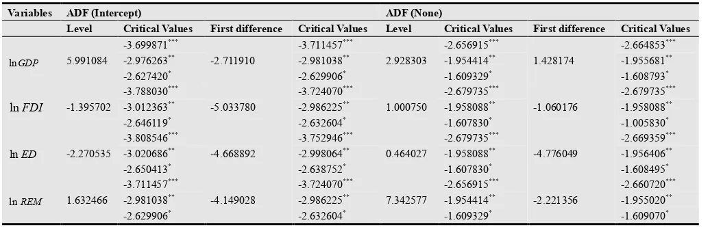
Table: 1 shows the Augmented Dickey - Fuller (ADF) t-statistics and critical values for two cases of the test equation (with constant and without constant). The null hypothesis is that the variable has unit root i.e. non-stationary. The decision rule is as follows:

If t-statistics (t*) > ADF critical value, we fail to reject null hypothesis, i.e., unit root exists (variable is non-stationary).

If t-statistics (t*) < ADF critical value, reject null hypothesis, i.e., unit root does not exists (variable is stationary).

Table 1. Augmented Dickey – Fuller (ADF) Unit Root Test

Variables ADF (Intercept) ADF (None)

Level Critical Values First difference Critical Values Level Critical Values First difference Critical Values

GDP

ln 5.991084

-3.699871***

-2.711910

-3.711457***

2.928303

-2.656915***

1.428174

-2.664853***

-2.976263** _-2.981038** _-1.954414** _-1.955681**

-2.627420* _-2.629906* _-1.609329* _-1.608793*

FDI

ln -1.395702

-3.788030***

-5.033780

-3.724070***

1.000750

-2.679735***

-1.060176

-2.679735***

-3.012363** _-2.986225** _-1.958088** _-1.958088**

-2.646119* _-2.632604* _-1.607830* _-1.005830*

ED

ln -2.270535

-3.808546***

-4.668892

-3.752946***

0.464027

-2.679735***

-4.776049

-2.669359***

-3.020686** _-2.998064** _-1.958088** _-1.956406**

-2.650413* _-2.638752* _-1.607830* _-1.608495*

REM

ln 1.632466

-3.711457***

-4.149028

-3.724070***

7.342577

-2.656915***

-2.221356

-2.660720***

-2.981038** _-2.986225** _-1.954414** _-1.955020**

-2.629906* _-2.632604* _-1.609329* _-1.609070*

N.B: The null hypothesis is that the variable is non-stationary. A variable is said to be non- stationary if the absolute value of ADF is lower than the critical value or the test-statistics of ADF is greater than the critical value. Superscripts***, ** and * indicate Critical values at 1%, 5% & 10% level of significance.

At level with intercept, the computed ADF test-statistics

(5.991084) of lnGDP is greater than critical values (-3.699871, -2.976263 and -2.627420 at 1%, 5% and 10%

significant level, respectively), so we can not reject null

difference, the computed ADF test-statistics is smaller than the critical values of both case (Intercept and none) and we can reject the null hypothesis that variable has a unit root. That means the first-difference of lnGDP becomes stationary. So the variable is non-stationary and it is integrated of order one I(1).

The Augmented Dickey-Fuller test statistics at level with intercept is (-1.395702) for the variable log of foreign direct investment (ln FDI) is larger than the critical values (-3.788030, -3.012363 and -2.646119 at 1%, 5% and 10% significant level, respectively) so we fail to reject the null hypothesis (non-stationary). That means the log FDI (ln FDI) series has unit root problem and ln FDI is non-stationary series. It is also non stationary when we used no intercept and no trend (none) at level. To make the series stationary we have to take the first difference and found ADF test-statistics is smaller than critical value for both the cases (Intercept, None). Thus, we conclude that the variable is non-stationary and it is integrated of order one I(1).

Similarly we got the series log ED (ln ED) and log REM (ln REM) with both intercept and non at level have the unit root problem that means they (the series) are non-stationary. As in previous cases if we take the first difference for both

log ED (ln ED) and log REM (ln REM) then for both intercept and none cases we can overcome the unit root problem that means the series become stationary. So the variables are non-stationary and they (the series) are integrated of order one I(1).

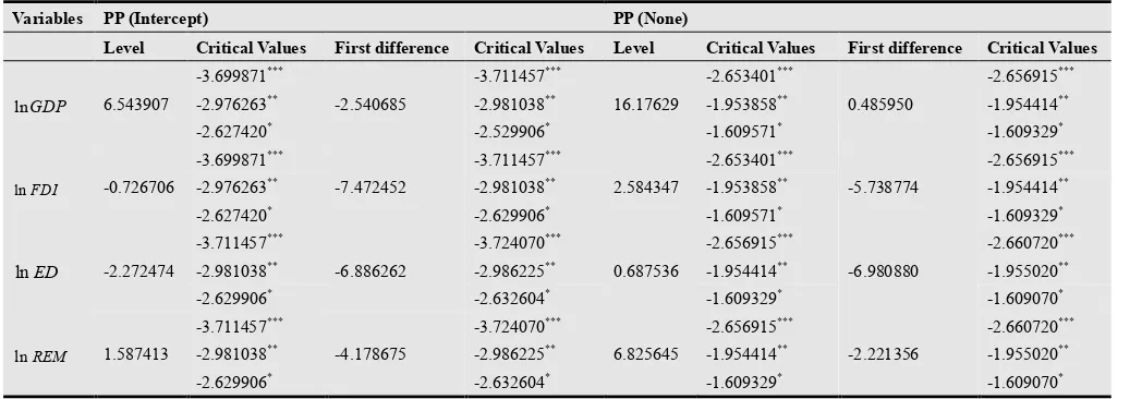
3.2. The Phillips-Perron (PP) Unit Root Test

The alterative test for existence of a unit root in the residuals of the cointegrating regression is that suggested by Phillips (1987) and extended by Perron (1988) and Philips and Perron (1988). An important assumption of the DF test is that the error terms ut are independently and identically

distributed. The ADF test adjusts the DF test to take care of possible serial correlation in the error terms by adding the lagged difference terms of the regressed. Phillips and Perron (1988) use nonparametric statistical methods to take care of the serial correlation in the error terms without adding lagged difference terms. The asymptotic distribution of the PP test is same as the ADF test statistics. The Phillips-Perron unit root test results for the logarithms of level and first difference of both the variables are present in Table: 2

Table 2. Phillips-Perron Unit Root Test

Variables PP (Intercept) PP (None)

Level Critical Values First difference Critical Values Level Critical Values First difference Critical Values

GDP

ln 6.543907

-3.699871***

-2.540685

-3.711457***

16.17629

-2.653401***

0.485950

-2.656915***

-2.976263** _-2.981038** _-1.953858** _-1.954414**

-2.627420* _-2.529906* _-1.609571* _-1.609329*

FDI

ln -0.726706

-3.699871***

-7.472452

-3.711457***

2.584347

-2.653401***

-5.738774

-2.656915***

-2.976263** _-2.981038** _-1.953858** _-1.954414**

-2.627420* -2.629906* -1.609571* -1.609329*

ED

ln -2.272474

-3.711457***

-6.886262

-3.724070***

0.687536

-2.656915***

-6.980880

-2.660720***

-2.981038** _-2.986225** _-1.954414** _-1.955020**

-2.629906* _-2.632604* _-1.609329* _-1.609070*

REM

ln 1.587413

-3.711457***

-4.178675

-3.724070***

6.825645

-2.656915***

-2.221356

-2.660720***

-2.981038** _-2.986225** _-1.954414** _-1.955020**

-2.629906* _-2.632604* _-1.609329* _-1.609070*

N.B: The null hypothesis is that the variable is non-stationary. A variable is said to be non- stationary if the absolute value of PP is lower than the critical value or the test-statistics of PP is greater than the critical value. Superscripts***, ** and * indicate Critical values at 1%, 5% & 10% level of significance.

The result of the Phillips-Perron unit root tests are presented in Table 1.2. we have tested all four variables- gross domestic product (GDP), foreign direct investment (FDI), external debt (ED) and remittance (REM). All variables are used in logarithmic form (ln GDP, ln FDI, ln ED, and ln REM). The bandwidth is automatically selected by Newey-West Bandwidth. The null hypothesis is that the variable has unit root i.e. non-stationary.

The decision rule as follows:

If t-statistics (t*) > PP critical value, not reject null hypothesis, i.e., unit root exists (variable is non-stationary). If t-statistics (t*) < PP critical value, reject null hypothesis, i.e., unit root does not exists (variable is stationary).

From the Table: 2, we found that the PP test-statistics for all variables at level are not significant irrespective of whether it is run with intercept or no trend no intercept (none). The test-statistics of these four series are not significant at 1%, 5% and 10% levels. Thus it can be concluded that all the data series ln GDP, ln FDI, ln ED and ln REM contained unit root at level. But if we take the first difference of all series, we found that they become stationary for all cases [with intercept and no trend no intercept (none)]. That means all the variables are integrated of order one in level and zero in first difference.

Phillips-Perron (PP) unit root test is same as the results of Augmented Dickey-Fuller (ADF) test.

Generally we know that if R-squared value of OLS is 65% it shows the model is moderately adequate and if the R square value is more than 80% then it shows that accuracy of the model is very good. We also know that if P value of an individual variable is less than 5% then that variable is statistically significant. And again we also know that if the residual of an OLS regression model free from serial correlation, heteroskedasticity and if the residuals are normally distributed then the model is fitted well.

Table 3. Result of OLS regression

Dependent Variable: LGDP Method: Least Squares Date: 11/18/14 Time: 02:21 Sample (adjusted): 1986 2012

Included observations: 27 after adjustments

Variable Coefficient Std. Error t-Statistic Prob.

C 18.21949 0.527063 34.56797 0.0000

LFDI 0.017672 0.006893 2.563723 0.0174

LED -0.092219 0.030066 -3.067175 0.0055

LREM 0.367293 0.019362 18.96940 0.0000

R-squared 0.992242 Mean dependent var 24.53360

Adjusted R-squared 0.991230 S.D. dependent var 0.404050 S.E. of regression 0.037840 Akaike info criterion -3.574971

Sum squared resid 0.032932 Schwarz criterion -3.382995

Log likelihood 52.26211 Hannan-Quinn criter. -3.517887

F-statistic 980.4992 Durbin-Watson stat 1.230655

Prob(F-statistic) 0.000000

Table 3 represent that R-squared value is 0.992242 that means 99% it show that model is accurate. The P values of all the independent variables are less than 5%, which means all coefficients of the independent variables are statistically significant and can influence the dependent variable GDP. The coefficient value shows the relationship of dependent variable and independent variable; here we got positive relationship with GDP, FDI and REM but negative relationship between GDP and ED.

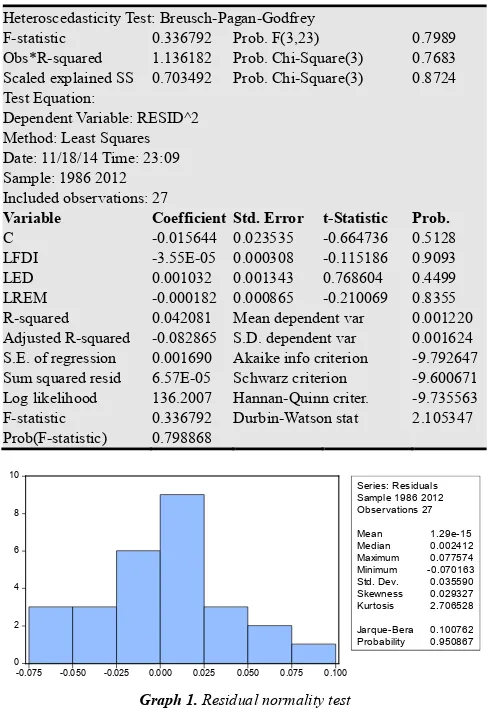
We also found that residual of our OLS model is not serially correlated, homoscedastic and the residual of the OLS is normally distributed (Results are the attached to the annex in table: 5, 6, Graph-1).So we can say that our model is fitted well.

lnGDP= α+ β1 (lnFDI) +β2(lnED) +β3 (lnREM) +eye

= 18.21949+0.017672 (lnFDI)-0.092219 (lnED) +0.367293 (lnREM)

LGDP does Granger cause LREM because its P value is less than 5% and LFDI does not Granger cause LED, LED does not Granger cause LFDI, LGDP does not Granger Cause LED, LED does not Granger Cause LGDP, LREM does not Granger Cause LED, LED does not Granger Cause LREM, LGDP does not Granger Cause LFDI, LFDI does not Granger Cause LGDP, LREM does not Granger Cause LFDI, LFDI does not Granger Cause LREM, LREM does not

Granger Cause LGDP because all of these pair has P value more than 5%.

Table 4. Granger Causality Tests

Pairwise Granger Causality Tests

Date: 11/19/14 Time: 00:45

Sample: 1986 2013

Lags: 2

Null Hypothesis: Obs F-Statistic Prob.

LFDI does not Granger Cause LED 25 1.20401 0.3208

LED does not Granger Cause LFDI 0.64315 0.5362

LGDP does not Granger Cause LED 25 1.82492 0.1871

LED does not Granger Cause LGDP 0.92923 0.4112

LREM does not Granger Cause LED 25 2.03429 0.1570

LED does not Granger Cause LREM 0.91678 0.4160

LGDP does not Granger Cause LFDI 26 2.86599 0.0793

LFDI does not Granger Cause LGDP 0.07279 0.9300

LREM does not Granger Cause LFDI 25 1.34109 0.2841

LFDI does not Granger Cause LREM 1.64452 0.2182

LREM does not Granger Cause LGDP 25 2.04406 0.1557

LGDP does not Granger Cause LREM 5.13364 0.0159

3.3. Analysis of the Results

OLS method has been applied to the annual data of 1986 to 2013 for Bangladesh on the variables Gross domestic product (GDP) as dependent variable and foreign direct investment (FDI), external debt (ED) and remittance (REM) are as independent variable. The results are significant for all the variables; but they do not affect the GDP in same way. Both FDI and REM affect the GDP positively, where as ED affect the GDP negatively. On the basis of the results of the OLS it can be concluded that two hypothesis (FDI has positive relationship with GDP, Remittances has positive relationship with GDP) are accepted, except the hypothesis ED has positive relationship with GDP.

The external debt is not on increase in the Bangladesh economy. The external debt shows negative relationship with GDP because of too much interest on external debt, strict restriction of use of debt money. On the top of these international authority imposes different restrictive policy on issuing debt. International lenders group imposes policy to bring structural change in the economy which is not appropriate for the economy. Sometimes the lenders groups imposes conditions like where to use the loan, how to use the loan. In many cases they determine from where to purchases raw materials, technology, technical human resources; which increases the cost of the project. Shield out the benefits of the projects. Finally we can say, higher current account and fiscal deficits are among major reasons for higher debt burden on these countries. When debt exceeds a specified limit then debt servicing can be a burden for the country.

4. Conclusion and Recommendations

economic growth in the Bangladesh. FDI brings prosperity to the Bangladesh through technology transfer, increasing volume of exports, enhancing job opportunities and increasing the government revenue. Similarly remittance also contribute to the economic growth throw injecting foreign currency consequently stagnating the foreign exchange reserve in the country and contributing to the capital formation in Bangladesh. ED could also be the alternative sources of minimizing the gap between the savings and capital need if it could use as according to the need and structure of the economy.

Bangladesh should reinforce its infrastructure facilities, and improve the quality of services. Furthermore, a consistent incentive package should be implemented which may include fiscal measures (such as rationalization of Para tariffs, elimination of non-tariff barriers), financial measures (such as reducing interest rates, access to financing), and institutional measures (such as enhancement of competitiveness through capacity building) to attract the FDI.

To increase the REM Bangladesh government should take the measures to enhance the human resources quality and should take the policy to bring the Bangladeshi foreign worker and nonresident Bangladeshi’s money through proper channel so that these REM can be used according to the national plan.

ED shows a negative relationship with GDP. So the authority should use external debt carefully and considering the needs, structural adjustment. Fiscal policy’s gap should minimize by using internal debt from money market and long term projects should finance through capital market.

Annex

Table 5. Serial correlation test

Breusch-Godfrey Serial Correlation LM Test:

F-statistic 2.758491 Prob. F(2,21) 0.0864

Obs*R-squared 5.617477 Prob. Chi-Square(2) 0.0603

Test Equation:

Dependent Variable: RESID Method: Least Squares Date: 11/18/14 Time: 23:01 Sample: 1986 2012 Included observations: 27

Presample missing value lagged residuals set to zero.

Variable Coefficient Std. Error t-Statistic Prob.

C -0.189031 0.551993 -0.342452 0.7354

LFDI 0.002028 0.007042 0.287987 0.7762

LED 0.012652 0.029495 0.428956 0.6723

LREM -0.005060 0.019176 -0.263881 0.7944

RESID(-1) 0.518512 0.231916 2.235780 0.0364

RESID(-2) -0.327123 0.250968 -1.303447 0.2065

R-squared 0.208055 Mean dependent var 1.29E-15

Adjusted R-squared 0.019496 S.D. dependent var 0.035590 S.E. of regression 0.035241 Akaike info criterion -3.660086

Sum squared resid 0.026080 Schwarz criterion -3.372122

Log likelihood 55.41116 Hannan-Quinn criter. -3.574459

F-statistic 1.103397 Durbin-Watson stat 1.869645

Prob(F-statistic) 0.388165

Table 6. Heteroscedasticity test

Heteroscedasticity Test: Breusch-Pagan-Godfrey

F-statistic 0.336792 Prob. F(3,23) 0.7989

Obs*R-squared 1.136182 Prob. Chi-Square(3) 0.7683

Scaled explained SS 0.703492 Prob. Chi-Square(3) 0.8724 Test Equation:

Dependent Variable: RESID^2 Method: Least Squares Date: 11/18/14 Time: 23:09 Sample: 1986 2012 Included observations: 27

Variable Coefficient Std. Error t-Statistic Prob.

C -0.015644 0.023535 -0.664736 0.5128

LFDI -3.55E-05 0.000308 -0.115186 0.9093

LED 0.001032 0.001343 0.768604 0.4499

LREM -0.000182 0.000865 -0.210069 0.8355

R-squared 0.042081 Mean dependent var 0.001220

Adjusted R-squared -0.082865 S.D. dependent var 0.001624 S.E. of regression 0.001690 Akaike info criterion -9.792647 Sum squared resid 6.57E-05 Schwarz criterion -9.600671 Log likelihood 136.2007 Hannan-Quinn criter. -9.735563

F-statistic 0.336792 Durbin-Watson stat 2.105347

Prob(F-statistic) 0.798868

0 2 4 6 8 10

-0.075 -0.050 -0.025 0.000 0.025 0.050 0.075 0.100

Series: Residuals Sample 1986 2012 Observations 27 Mean 1.29e-15 Median 0.002412 Maximum 0.077574 Minimum -0.070163 Std. Dev. 0.035590 Skewness 0.029327 Kurtosis 2.706528 Jarque-Bera 0.100762 Probability 0.950867

Graph 1. Residual normality test

References

[1] Agrawal, G. and A. Khan, 2011, “Impact on FDI on GDP: A

Comparative Study of China and India” International Journal

of Business and Management, 6(10), P: 71-79.

[2] Alfaro, L. (2003), “Foreign Direct Investment and Growth:

Does the Sector Matter?” Mimeo. Boston, MA: Harvard

Business School.

[3] Bos, H.C., Sanders, M. and Secchi C. (1974) “Private Foreign Investment in Developing Countries: A Quantitative Study on

the Macroeconomic Effects”, Dardrecht: Reidel.

[4] Caves, R. E. (1974) “Multinational firms, Competition and

Productivity in Host Country Markets”, Economica , 41,

176-93.

[5] Chowdhury, A. and G. Mavrotas (2005), “FDI and growth: A

causal relation”, WIDER Research Paper. Finland: UNU

World Institute for Development Economics Research. [6] Crespo, Nuno and Fontoura, Maria Paula (2007).

“Determinant Factors of FDI Spillovers- What do we really

know?” World Development, Vol. 35, No. 3, pp 410-425.

[7] Duasa, J (2007), “Malaysian Foreign Direct Investment and

Growth: Does Stability Matters”. Journal of Economic

[8] Granger, C. (1981), “Some Properties of Time Series Data

and Their use in Econometric Model Specification.” Journal

of Econometrics, 16. P: 121-130.

[9] Gujrati, N. Damodar. (2003) “Basic Econometrics” (4th

Editions) McGraw-Hill/Irwin.

[10] Hayami, Yujiro (2001). “Development Economics: From

Poverty Alleviation to the Wealth of Nations”, 2nd Edition.

New York: Oxford University Press.

[11] Kamaly, A. 2002. “Evaluation of FDI Flows into the MENA

Region.” Working Paper Series. Cairo, Egypt: Economic

Research Forum.

[12] Kukeli, Agim, Chuen-Mei Fan and Liang-Shing Fan (2006),

“FDI and growth in transition economies: Does the mode of

transition make a difference?” RISEC, 53(3): 302-322.

[13] Mohammed S. and Sidiropoulos (2010), “Do Worker Remittances Affect Growth: Evidence from Labor Exporting

MENA Countries?” International Research Journal of Finance

and Economics 46(2010):181-194.

[14] Phillips, P.C.B and P. Perron (1988) “Testing for a Unit Root

in Time Series Regression” Biometrika, 75, P: 335-346.

[15] Pradhan, R. P. (2009), “The FDI-led-growth hypothesis in ASEAN-5 countries: Evidence from cointegrated panel

analysis”, International Journal Business and Management,

4(12): 153-164.

[16] Prebisch, R. (1968) “Development Problems of the Peripheral

Countries and the Terms of Trade, in: James D.” Theberge, ed.

Economics of Trade and Development. New York: John Wiley and Sons Inc.

[17] Reza, S. Rashid, M.A. and Alam, M (1987). “Private

Investment in Bangladesh”, The University Press Ltd.:Dhaka.

[18] Saltz, S. (1992) “The Negative Correlation between Foreign Direct Investment and Economic Growth in the Third World:

Theory and Evidence,” Rivista Internazionale di Scienze

Economiche e Commerciali, 39, 617-633.

[19] Samimi, A. J., Zeinab Rezanejad and Faezeh Ariani (2010),

“Growth and FDI in OIC Countries”, Australian Journal of

Basic and Applied Sciences, 4(10): 4883-4885.

[20] Singer, H.W. (1950) “The Distribution of Gains between

Investing and Borrowing Countries”, American Economic