http://www.sciencepublishinggroup.com/j/pamj doi: 10.11648/j.pamj.20170605.11
ISSN: 2326-9790 (Print); ISSN: 2326-9812 (Online)
On One Justification on the Use of Hybrids for the Solution
of First Order Initial Value Problems of Ordinary Differential
Equations
Kamoh Nathaniel Mahwash
1, Gyemang Dauda Gyang
2, Soomiyol
Mrumun Comfort
31
Department of Mathematics/Statistics, Bingham University, Karu, Nigeria
2Department of Mathematics and Computer Science, Benue State University, Makurdi, Nigeria 3Department of Mathematics/Statistics, Plateau State Polytechnic, BarkinLadi, Nigeria
Email address:
[email protected] (K. N. Mahwash), [email protected] (G. D. Gyang), [email protected] (S. M. Comfort)
To cite this article:
Kamoh Nathaniel Mahwash, Gyemang Dauda Gyang, Soomiyol Mrumun Comfort. On One Justification on the Use of Hybrids for the Solution of First Order Initial Value Problems of Ordinary Differential Equations. Pure and Applied Mathematics Journal.
Vol. 6, No. 5, 2017, pp. 137-143. doi: 10.11648/j.pamj.20170605.11
Received: September 7, 2017; Accepted: September 18, 2017; Published: October 11, 2017
Abstract:
This paper is aimed at discussing and comparing the performance of standard method with its hybrid method of the same step number for the solution of first order initial value problems of ordinary differential equations. The continuous formulation for both methods was obtained via interpolation and collocation with the application of the shifted Legendre polynomials as approximate solution which was evaluated at some selected grid points to generate the discrete block methods. The order, consistency, zero stability, convergent and stability regions for both methods were investigated. The methods were then applied in block form as simultaneous numerical integrators over non-overlapping intervals. The results revealed that the hybrid method converges faster than the standard method and has minimum absolute error values.Keywords:
Hybrid Method, Collocation, Interpolation, Shifted Legendre Polynomials Approximation, Continuous Block Method, Order, Consistency, Zero Stability, Convergent1. Introduction
Most physical phenomena in science and engineering used mathematical models to help in the understanding of the physical world problems. These models often yield equations that contain some derivatives of an unknown function of one or several variables. Such equations are called differential equations. Differential equations play an important role in the modeling of physical problems arising from almost every discipline of study such as economics, medicine, psychology, operation research, space technology and even in areas such as biology and astronomy.
Interestingly, differential equations arising from the modeling of such physical phenomena often are very difficult or impossible to solve analytically. Hence, the need for the development of numerical methods to obtain approximate solutions becomes inevitable.
Many scholars have worked extensively on the solution of differential equations. These authors proposed different
methods ranging from predictor corrector method to block method using different polynomials as basis functions evaluated at some desired points.
In this work, two types of block methods are proposed, the first is the five-step standard block method and the second is the five-step hybrid method with four off- grid points, using the shifted Legendre polynomials evaluated at some grid and off-grid points to give the needed discrete schemes.
Consider a numerical method for solving general first order initial value problems of ordinary differential equations of the form:
0
( , ), (0)
y′ = f x y y =y (1)
the Continuous implicit hybrid one step methods for the solution of initial value problems of general second order ordinary differential equations. [5], introduced the application of two step continuous hybrid Butcher’s method in block form for the solution of first order initial value problems; this approach eliminates requirements for a starting value. [2], introduced a new hybrid method for systems of stiff equations. [11], developed a new Butcher type two-step block hybrid multistep method for accurate and efficient parallel solution of ordinary differential equations. [1], used hybrid formula of order four to generate starting values for Numerov method. [3], developed linear multistep hybrid methods with continuous coefficients for solving stiff ordinary differential equations. [10], introduced a hybrid linear collocation multistep scheme for solving first order initial value problems of ordinary differential equations. [9], developed a three step implicit hybrid linear multistep method for the solution of third order ordinary differential equations.
2. Derivation of the Method
In this section, two methods are developed namely five-step block method and five-five-step with three off-grid points, by interpolating and collocating at some selected points.
Consider the shifted Legendre approximation of the form
0
( ) i i( )
i
y x C P t
φ
=
=
∑
(2)where = + − 1, and are interpolation and collocation points. The first derivative of (2) gives
0
( ) i i( )
i
y x C P t
φ
=
′ =
∑
′ (3)substituting (3) in (1), to get
0
( , ) i i( )
i
f x y C P t
φ
=
′
=
∑
(4)2.1. Five Step Method
Interpolating (2) at and collocating (3) at , , , , and gives the system of nonlinear equations of the form
AX = B (5)
where
0 1 2
1 1 1 1
0 1 2
1 1 1 1
0 1 2
1 1 1 1
0 1 2
1 1 1 1
0 1 2
1 1 1 1
0 1 2
1 1 1
0 1 0
(4 ) (4 ) (4 ) . . . (4 )
. . .
(0) (0) (0) . . (0)
.. .
( ) ( ) ( ) . . . ( )
(2 ) (2 ) (2 ) . . . (2 )
(3 ) (3 ) (3 ) . . . (3 )
. .
(4 ) (4 ) (4 ) . (4 )
. .
(5 ) (5 )
p h p h p h p h
p p p p
p h p h p h p h
p h p h p h p h
A
p h p h p h p h
p h p h p h p h
p h p h p
φ
φ
φ
φ
φ
φ =
1
(5 )h . . . pφ(5 )h
0
4
1
1
2
3
5
. . .
, . . .
. .
.
n
n
n
n
n
n
c
y
c
f
f
X B f
f
f cφ
+
+
+
+
+
= =
Solving for the ′ using inverse of a matrix method and substituting in (2) gives the continuous formulation
4 5
0 0
( ) j( ) n j j( ) n j
j j
y x α x y + h β x f +
= =
=
∑
+∑
(6)where
= = = = 0, = 1
= −14
45ℎ −
17
96ℎ ⁴ +
1
40ℎ ⁵ −
1
720ℎ ⁶
= −64
45ℎ +
5
2ℎ ² −
77
36ℎ ³ +
71
96ℎ ⁴ −
7
60ℎ ⁵ +
1
144ℎ ⁶
= − 8
15ℎ −
5
2ℎ ² −
59
48ℎ ⁴ −
1
72ℎ ⁶ +
13
60ℎ ⁵ +
107
= −64
45ℎ +
5
3ℎ ² −
13
6ℎ ³ +
49
48ℎ ⁴ −
1
5ℎ ⁵ +
1
72ℎ ⁶
= 11
120ℎ ⁵ −
14
45ℎ +
61
72ℎ ³ −
1
144ℎ ⁶ −
41
96ℎ ⁴ −
5 8ℎ ² = ( − )(* + + ,)(- −) (. ++ (/
) (7)
Evaluating (6) with coefficients (7) at , , , and with = ( − ) the following discrete schemes is respectively obtained as;
3 = 3 −14
45ℎ −
64
45ℎ −
8
15ℎ −
64
45ℎ −
14
45ℎ
3 = 3 + 3
160ℎ −
69
160ℎ −
87
80ℎ −
87
80ℎ −
69
160ℎ +
3
160ℎ
3 = 3 + 1
90ℎ −
17
45ℎ −
19
15ℎ −
17
45ℎ +
1
90ℎ
3 = 3 + 11
1440ℎ −
77
1440ℎ +
43
240ℎ −
511
720ℎ −
637
1440ℎ +
3
160ℎ
3 = 3 +
) ℎ − +
ℎ +
+ ℎ − ℎ +
+
ℎ + ,
44ℎ (8) 2.2. Five Step Method with Three Off-Grid Points
Interpolating (2) at and collocating (3) at , , , , , 5
-, 6 *
, 5.
and gives a system of nonlinear equations of the form
AX = B (9)
where
0 1 2
1 1 1 1
0 1 2
1 1 1 1
0 1 2
1 1 1 1
0 1 2
1 1 1 1
0 1 2
1 1 0 1 1 0 1 0 1 0
(4 ) (4 ) (4 ) . . . (4 )
. . .
(0) (0) (0) . . (0)
.. .
( ) ( ) ( ) . . . ( )
(2 ) (2 ) (2 ) . . . (2 )
(3 ) (3 ) (3 ) . . . (3 )
(4 ) (4
13 3 9 2 14 3
p h p h p h p h
p p p p
p h p h p h p h
p h p h p h p h
p h p h p h p h
A p h p
p h p h p h φ φ φ φ φ = 1 1 2
1 1 1
1 1
1 1 1
1 2
1 1 1
1 2
1 1 1 1
0 1 0
(4 )
) (4 )
13 13 13
3 3 3
. .
.
. .
9 9 9
2 2 2
14 14 14
3 3 3
(5 ) (5 ) (5 ) . . . (5 )
p h
h p h
p h p h p h
p h p h p h
p h p h p h
p h p h p h p h
φ φ φ φ φ 0 4 1 1 2 3 4 13 3 9 2 14 3 5 . . . . . . . , . . . . n n n n n n n n n n c y c f f f f f X B f f f f cφ + + + + + + + + + = =
1 0 0 ( ) ( ) ( ) ( ) i i i k k
j n j j n j n
j j
y x x y h x f h ω x f ω
ω
α β β
−
+ + +
= =
=
∑
+∑
+∑
(10)where
7 = 5, 8 = , 8 =,, 8 = , = = = = 0 and = 1
= − 351518 1289925ℎ −
48331
32760ℎ ² + 87149
73710ℎ2 ³ −
16811
29120ℎ3 ⁴ +
88541
491400ℎ4 ⁵ −
7123
196560ℎ5 ⁶ +
1567
343980ℎ6 ⁷ −
19
58240ℎ7 ⁸ +
1
98280ℎ8 ⁹
= 3
896ℎ+ ⁸ −
31951
4620ℎ ³ −
1
9240ℎ4 ⁹ −
212552
121275ℎ +
15689
3696ℎ ⁴ +
117
22ℎ ² −
140117
92400ℎ ⁵ +
7393
22176ℎ ⁶ −
5773
129360ℎ) ⁷
= 10016
11025ℎ −
117
8ℎ ² +
40141
1680ℎ ³ −
228173
13440ℎ ⁴ +
56431
8400ℎ ⁵ −
3211
2016ℎ ⁶ +
2657
11760ℎ) ⁷ −
159
8960ℎ+ ⁸ +
1
1680ℎ4 ⁹
=91
2ℎ ² −
31672
4725 ℎ −
42871
540ℎ ³ +
14603
240ℎ ⁴ −
92887
3600ℎ ⁵ −
4891
5040ℎ) ⁷ +
1871
288ℎ ⁶ +
51
640ℎ+ ⁸ −
1
360ℎ4 ⁹
=19454
315 ℎ −
4095
8ℎ ² +
11059
12ℎ ³ −
141121
192ℎ ⁴ +
39097
120ℎ ⁵ −
12361
144ℎ ⁶ +
563
42ℎ) ⁷ −
147
128ℎ+ ⁸ +
1
24ℎ4 ⁹
5
-=59049
26ℎ ² −
4391496
15925 ℎ −
7494849
1820ℎ ³ +
4826709
1456ℎ ⁴ +
1154007
2912ℎ ⁶ −
3195207 50960ℎ) ⁷ −
729
3640ℎ4 ⁹ +
63423
11648ℎ+ ⁸ −
54082323
36400ℎ ⁵
6 *
=35618816
99225 ℎ −
26624
9ℎ ² +
15254528
2835ℎ ³ −
456704
105ℎ ⁴ +
9257216
4725ℎ ⁵ −
99328
189ℎ ⁶ +
553472
6615ℎ) ⁷ −
256
35ℎ+ ⁸ +
256
945ℎ4 ⁹
5.
-=767637
616ℎ ² −
2035368
13475 ℎ −
14003361
6160ℎ ³ +
90907029
49280ℎ ⁴ −
25712559
30800ℎ ⁵ +
554769
2464ℎ ⁶ −
1554957 43120ℎ) ⁷ +
28431
8960ℎ+ ⁸ −
729
6160ℎ4 ⁹
= ,
+ ℎ − 4 ,
( ² + , ) (* ³ −
, (- + )+ + (. − ,+ (/ )+ )4 (<
+− ) (=
4+ (>
, (11)
Evaluating (10) with coefficients (11) at , , , , 5
-, 6 *
, 5.
and with = ( − ) the following discrete schemes are respectively obtained as;
3 = 3 − 351518
1289925ℎ −
212552
121275ℎ +
10016
11025ℎ −
31672
4725 ℎ +
19454
315 ℎ +
15592
1575 ℎ
+35618816
99225 ℎ 6*
−4391496
15925 ℎ 5-
-− 2035368
13475 ℎ 5.
-3 = 32951
6115200ℎ + 3 −
568893
1724800ℎ −
459807
313600ℎ +
1189
22400ℎ −
50499
4480 ℎ −
34107
22400ℎ
−212224
3675 ℎ 6*
+92569149
2038400 ℎ 5-
-+ 82333989
3449600 ℎ 5.
-3 = 3 − 247
396900ℎ +
43
3675ℎ −
3509
9800ℎ −
6701
4725ℎ +
871
420ℎ +
69
175ℎ +
1466368
99225 ℎ 6*
−13851
1225 ℎ 5-
-−60507
9800 ℎ 5.
-3 = 14669
165110400ℎ + 3 −
20869
15523200ℎ +
36329
2822400ℎ −
202169
604800ℎ −
100187
40320 ℎ −
31411
201600ℎ
−745216
99225 ℎ 6*
+13557213
2038400 ℎ 5-
-+9737253
3449600ℎ 5.
-3
5
-= 690797
1083 289334400ℎ + 3 −
910757
101 847715200ℎ +
1336457
18 517766400ℎ −
2512217
3968092800ℎ +
31844549
− 3364243
1322697600ℎ −
134364928
651015225ℎ 6*
+19955023
55036800ℎ 5-
-+ 5577703
93139200ℎ 5.
-3 6
*
= 24863
42 268262400ℎ + 3 −
32833
3973939200ℎ +
48323
722534400ℎ −
91493
154828800ℎ +
1220071
10321920ℎ
− 115447
51609600ℎ −
21389
198450ℎ 6*
+231041241
521830400ℎ 5-
-+ 43797591
883097600ℎ 5.
-3 5.
-= 22037
33 852791700ℎ + 3 −
7253
795685275ℎ +
42467
578680200ℎ −
19853
31000725ℎ +
993749
8266860ℎ
− 29107
10333575ℎ +
7757824
651015225ℎ 6*
+180667
429975ℎ 5-
-+ 342733
2910600ℎ 5.
-3 = 3 − 179
165110400ℎ +
73
5174400ℎ −
31
313600ℎ +
359
604800ℎ +
1079
13440ℎ +
1989
22400ℎ −
61184
99225ℎ 6*
+
,)) +
4 ℎ 5-- + 4, +
,) ℎ 5.- (12)
3. Analysis of the Method
In this section the error constant, order, consistency, zero stability, convergent and region of absolute stability of the schemes generated are discussed.
3.1. Order and Error Constant
Expanding (8) and (12) in Taylor’s series and collecting like terms in powers of ℎ, the order and error constant are respectively obtained as follows;
Table 1. Order and Error Constants of the Discrete Schemes of the Block Method (8).
Scheme Order Error constant
3 6 += −5. 8035714 × 10⁻³
3 6 += −1. 3227513 × 10⁻³
3 6 += −4. 4808201 × 10⁻³
3 6 += 8. 46560850 × 10⁻³
3 6 += −1. 4269180 × 10⁻²
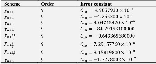
Table 2. Order and Error Constants of the Discrete Schemes of the Hybrid Block Method (12).
Scheme Order Error constant
3 9 = 4. 9057933 × 10⁻⁴
3 9 = −4. 255200 × 10⁻⁵
3 9 = 9. 04215420 × 10⁻⁶
3 9 = −84. 29153100000
3
5-- 9 = −0.643365680000
3 6
* 9 = 7. 29157760 × 10⁻⁸
3 5.
- 9 = 8. 15819800 × 10⁻⁸
3 9 = −1. 7278002 × 10⁻⁷
Hence the block methods are of order BC = 6, 9 and error constant of D+, D
respectively
3.2. Consistency
Following [8] and [6], the block methods are said to be consistent if they satisfy the following conditions:
(i) the order Ě ≥ 1
(ii) ∑JIK CI= 0
(iii) B(1) = BL(1)
(iv) BLL(1) = 2! N(1)
Where B(O) and N(O) are the first and second characteristics polynomials of the block method. According to [8] and [6], condition (i) above is a sufficient condition for the block methods to be consistent. Hence the block methods are consistent since Ě = 6, 9 > 1.
3.3. Zero Stability
The block methods are said to be zero stable if the roots
QR; O = 1, … , U of the first characteristic polynomial E(Q),
defined by
E(Q) = VW |QY − Z|
satisfies |QR| ≤ 1 and every root with |QR| = 1 has
multiplicity not exceeding two in the limit as ℎ → 0. Calculations from all available information revealed that the block methods (8) and (12) have the following roots respectively.
Q (Q − 1) = 0 and Q4(Q − 1) = 0
Hence the block methods are zero stable, since all roots with modulus one do not have multiplicity exceeding the order of the differential equation in the limit as ℎ → 0.
3.4. Convergence
According to [7], we can safely assert the convergence of the block methods (8) and (12)
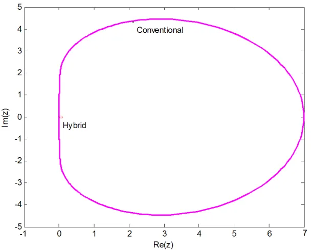
3.5. Region of Absolute Stability
Reformulating the block methods (8) and (12) as a General Linear Methods (GLM) containing a partition of matrices A, Band C and then substituting into the stability polynomial
O(] − Q) − ^. Using a MATLAB code based on the idea of
Figure 1. The regions of absolute stability for methods (8) and (12).
4. Numerical Illustrations
The following numerical experiments are performed with the aid of MAPLE 18 software package in order to further affirm the earlier established convergence of the methods.
Example 1
The ordinary differential equation
( )
5 , 0 1, 0 1, 0.01
y′ = y ≤ ≤x y = h= (13)
The exact solution is 3( ) = W _. ([12])
Example 2
The ordinary differential equation
( )
, 0 1, 0 0, 0.1
y′ = −x y ≤ ≤x y = h= (14)
The exact solution is 3( ) = + W`_− 1. ([10]).
Example 3
The ordinary differential equation
( )
2
1, 0 2, 0 0.5, 0.2
y′ = − +y x ≤ ≤x y = h= (15)
The exact solution is 3( ) = ( + 1) + 0.5W_,
([13])
Table 3. Absolute Error Values for Example 1 of Methods (8) and (12).
a Exact Solution Result of Method (8) Absolute error of (8) Result of Method (12) Absolute error of (12) 0.01 1.05127109637602 1.05127109638904 1.302 × 10` 1.05127109637607 5.0 × 10`
0.02 1.10517091807565 1.10517091808526 9.610 × 10` 1.10517091807569 4.0 × 10`
0.03 1.16183424272828 1.16183424274126 1.298 × 10` 1.16183424272835 7.0 × 10`
0.04 1.22140275816017 1.22140275816975 9.580 × 10` 1.22140275816017 0.00000000
0.05 1.28402541668774 1.28402541671072 2.298 × 10` 1.28402541668780 6.0 × 10`
0.06 1.34985880757600 1.34985880761687 4.087 × 10` 1.34985880757611 1.1 × 10`
0.07 1.41906754859326 1.41906754863098 3.772 × 10` 1.41906754859338 1.2 × 10`
0.08 1.49182469764127 1.49182469768462 4.335 × 10` 1.49182469764142 1.5 × 10`
0.09 1.56831218549017 1.56831218553052 4.035 × 10` 1.56831218549031 1.4 × 10`
0.10 1.64872127070013 1.64872127075914 5.901 × 10` 1.64872127070028 1.5 × 10`
Table 4. Absolute Error Values for Example 2 of Methods (8) and (12).
a Exact Solution Result of Method (8) Absolute error of (8) Result of Method (12) Absolute error of (12) 0.1 0.004837418035960 0.0048374169836170 1.05 × 10`, 0.0048374180358260 1.34 × 10`
0.2 0.018730753077982 0.0187307524576758 6.20 × 10` 0.0187307530778861 9.59 × 10`
0.3 0.040818220681718 0.0408182198857461 7.96 × 10` 0.0408182206816284 8.96 × 10`
0.4 0.070320046035639 0.0703200456495184 3.86 × 10` 0.0703200460355589 8.01 × 10`
0.5 0.106530659712633 0.106530658294696 1.42 × 10`, 0.106530659712561 7.20 × 10`
0.6 0.148811636094026 0.148811634172747 1.92 × 10`, 0.148811636093972 5.40 × 10`
0.7 0.196585303791410 0.196585302254268 1.54 × 10`, 0.196585303791371 3.90 × 10`
0.8 0.249328964117222 0.249328962584008 1.53 × 10`, 0.249328964117176 4.60 × 10`
0.9 0.306569659740599 0.306569658555933 1.85 × 10`, 0.306569659740559 4.00 × 10`
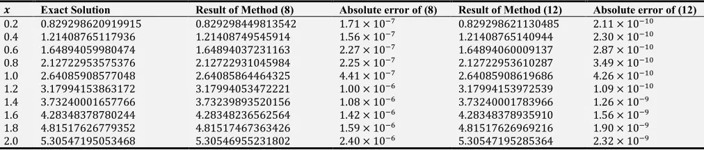
Table 5. Absolute Error Values for Example 3 of Methods (8) and (12).
a Exact Solution Result of Method (8) Absolute error of (8) Result of Method (12) Absolute error of (12) 0.2 0.829298620919915 0.829298449813542 1.71 × 10`+ 0.829298621130485 2.11 × 10`
0.4 1.21408765117936 1.21408749545914 1.56 × 10`+ 1.21408765140944 2.30 × 10`
0.6 1.64894059980474 1.64894037231163 2.27 × 10`+ 1.64894060009137 2.87 × 10`
0.8 2.12722953575376 2.12722931045984 2.25 × 10`+ 2.12722953610287 3.49 × 10`
1.0 2.64085908577048 2.64085864464325 4.41 × 10`+ 2.64085908619686 4.26 × 10`
1.2 3.17994153863172 3.17994053472221 1.00 × 10`) 3.17994153972539 1.09 × 10`
1.4 3.73240001657766 3.73239893520156 1.08 × 10`) 3.73240001783966 1.26 × 10`,
1.6 4.28348378780244 4.28348236562564 1.42 × 10`) 4.28348378935910 1.56 × 10`,
1.8 4.81517626779352 4.81517467363426 1.59 × 10`) 4.81517626969216 1.90 × 10`,
2.0 5.30547195053468 5.30546955231802 2.40 × 10`) 5.30547195285364 2.32 × 10`,
5. Discussion of Result
Two different methods for solving first order initial value problems of ordinary differential equations have been proposed in this work, the conventional or standard method and the hybrid method with the hybrid having more advantages over the conventional method the hybrid higher order and accuracy. The methods does not require developing separate predictors to implement this makes it simple and attractive for solving initial value problems of ordinary differential equations. A careful observation of Tables 1, 2 and 3 showed that both standard and hybrid methods performed well as their absolute error values are convergent, hence affirming the earlier established convergence of the methods. The hybrid method is useful as it reduces the step number of a method and still remains zero stable; in addition, the absolute error values presented in Tables 3, 4 and 5 indicated that the hybrid method performed better than the standard method when applied to stiff and non-stiff differential equations respectively. The results also revealed that the hybrid method converges faster than the standard method, since it has minimum absolute error values.
6. Conclusion
Justifying from the numerical calculations, it has been observed that the hybrid method performed well than the conventional method, it has also been established from the calculations that the hybrid method has high order and relatively small error constants than the conventional method. Finally, it has been established that hybrid methods gives better results than the standard methods when applied to either stiff or non-stiff initial value problems.
References
[1] Adee, S. O., Onumanyi, P., Sirisena, U. W. andYahaya, Y. A. (2005) Note on Starting the Numerov Method More Accurately by a Hybrid Formula of Order Four for Initial Value Problems. Journal of Computational and Applied Mathematics, 175: 369-373.
[2] Ademiluyi, R. A. (1987) New Hybrid Methods for Systems of Stiff Equations, Benin City, Nigeria: PhD Thesis, University of Benin.
[3] Akinfenwa, O. A., Jator, S. N. and Yao, N. M. (2011) Linear Multistep Hybrid Methods with Continuous Coefficients for Solving Stiff Ordinary Differential Equations, Journal of Modern Mathematics and Statistics, 5(2): 47-57.
[4] Anake, T. A. (2011). Continuous Implicit Hybrid One-Step Methods for the Solution of Initial Value Problems of Second Order Ordinary Differential Equations. Ogun State, Nigeria. PhD Thesis, Covenant University, Ota.
[5] Awari, Y. S., Abada, A. A., Emma, P. M. and Kamoh, N. M. (2013) Application of Two Step Continuous Hybrid Butcher’s Method in Block Form for the Solution of First Order Initial Value Problems. Natural and Applied Sciences, 4(4): 209-218. [6] Fatunla, S. O. (1988) Numerical Methods for Initial Value Problems for Ordinary Differential Equations USA, Academy press, Boston 295.
[7] Henrici, P. (1962) Discrete Variable Methods for ODE`s, New York, USA, John Wiley and Sons, (1962).
[8] Lambert, J. D. (1991) Numerical Methods for Ordinary Differential Equations, New York: John Wiley and Sons pp 293.
[9] Mohammed, U. and Adeniyi, R. B (2014) A Three Step Implicit Hybrid Linear Multistep Method for the Solution of Third Order Ordinary Differential Equations. General Mathematics Notes, 25(1): 62-74.
[10] Odejide, S. A. and Adenira, A. O. (2012) A Hybrid Linear Collocation Multistep Scheme For Solving First Order Initial Value Problems. Journal of the Nigerian Mathematical Society 31: 229-241.
[11] Serisina, U. W., Kumleng, G. M. and Yahaya, Y. A. (2004) A New Butcher Type Two-Step Block Hybrid Multistep Method for Accurate and Efficient Parallel Solution of Ordinary Differential Equations, Abacus Mathematics Series. 31: 1-7. [12] Yakusak, N. S., Emmanuel, S. and Ogunniran, M. O. (2015)
Uniform Order Legendre Approach for Continuous Hybrid Block Methods for the Solution of First Order Ordinary Differential Equations. IOSR Journal of Mathematics, 11(1): 09-14.