Gradients Weights improve Regression and Classification
Samory Kpotufe∗ [email protected]
Princeton University, Princeton, NJ
Abdeslam Boularias [email protected]
Rutgers University, New Brunswick, NJ
Thomas Schultz [email protected]
University of Bonn, Germany
Kyoungok Kim [email protected]
Seoul National University of Science & Technology (SeoulTech), Korea
Editor:Hui Zou
Abstract
In regression problems overRd, the unknown functionf often varies more in some coordinates than in others. We show that weighting each coordinateiaccording to an estimate of the variation off along coordinatei– e.g. theL1 norm of theith-directional derivative off – is an efficient way to significantly improve the performance of distance-based regressors such as kernel andk -NN regressors. The approach, termed Gradient Weighting (GW), consists of a first pass regression estimatefnwhich serves to evaluate the directional derivatives off, and a second-pass regression
estimate on the re-weighted data. The GW approach can be instantiated for both regression and classification, and is grounded in strong theoretical principles having to do with the way regression bias and variance are affected by a generic feature-weighting scheme. These theoretical principles provide further technical foundation for some existing feature-weighting heuristics that have proved successful in practice.
We propose a simple estimator of these derivative norms and prove its consistency. The pro-posed estimator computes efficiently and easily extends to run online. We then derive a classifica-tion version of the GW approach which evaluates on real-worlds datasets with as much success as its regression counterpart.
Keywords: Nonparametric learning, feature selection, feature weighting, nonparametric sparsity, metric learning.
1. Introduction
High-dimensional regression is the problem of inferring an unknown function f from data pairs
(Xi, Yi), i = 1,2, . . . n, where the input Xi belongs to a Euclidean subspace X ⊂ Rd and the
outputYi is a noisy version off(Xi). The problem is significantly harder for larger dimensiond,
and various pre-processing approaches have been devised over time to alleviate this so-calledcurse
of dimension. A simple and common approach is that of reducing the dimension of the inputX by
properly selecting a few coordinate-variables with the most influence on the problem. The general motivating assumption for these methods is that of (approximate)sparsity: the unknown function
∗. A significant part of this work was conducted when the authors were at the Max Planck Institute for Intelligent
f only varies along a few relevant coordinates in some subset R of [d] =. {1,2, . . . , d}, that is
f(X) =f X(R)
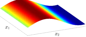
whereX(R)picks out the set of relevant coordinates. However, as illustrated by
Fig. 3, there are many real-world examples in whichf varies significantly along all coordinates, but varies more in some coordinates than in others. The natural approach in this case, implicit in some methods and heuristics (see Section 1.2), is toweighteach coordinate according to some measure of relevance learned from data. The learned coordinate-relevance would typically rely on various assumptions on the form off, for examplefmight be assumed linear.
In the case of nonparametric regression, where little is assumed about the form off, the ques-tion of how to properly weight coordinates has not received much theoretical attenques-tion. We present and analyze a simple approach termed Gradient Weighting (GW), consisting of weighting each co-ordinateiaccording to the (unknown) variation off alongi. To this end,f is estimated from data in a first pass asfn, wherefn serves to assess the coordinate-wise variation off and accordingly
weight the data; the transformed data is then used to re-estimatef in a second pass. This proce-dure can be iterated into a multi-pass proceproce-dure, although we only consider the two-pass version just described. We show that such weighting can be learned efficiently, is easily extended online, and can significantly improve the performance of distance-based regressors (e.g. kernel andk-NN regression) in real-world applications. Moreover the method easily extends to distance-based clas-sification methods such ask-NN classification and-NN classification.
The GW approach is grounded in strong theoretical principles (developed in Section 2) having to do with the way regression bias and variance are affected by the distribution of weights in a generic feature-weighting method. We argue in Section 2 that a good situation for distance-based regressors is one where the unknown functionf varies in a few coordinates more than in others, and the weights correlate with the variation off along coordinates. The theoretical intuition developed is kept general enough to also explain the practical success of some existing heuristics (see Section 6.2) which inherently learn weights that are correlated with the variation of the unknownf along coordinates. We validate the theoretical intuition in extensive experiments on many real-world datasets in Section 5.
There are many possible ways of capturing the variation of f along coordinates, thus the par-ticular instantiations of GW considered here are simply ones that work well in practice. Our aim is therefore not of arguing in favor of a particular way of capturing the coordinate-wise variation of
f, but rather that the general approach of weighting coordinates according to this variation offcan yield significant improvements in learning performance. The theoretical intuition developed in Sec-tion 2 uses, as a measure of the variaSec-tion off alongi, the maximum variation|fi0|sup,supx|fi0(x)|
along coordinatei. The maximum variation is a natural measure of smoothness and as such is intu-itive to argue about; however it is hard to estimate. Therefore, for practical instantiations of the GW approach, we instead measure the average variation offalong coordinates, specifically we estimate the normskfi0k1,µ=EX∼µ|fi0(X)|, whereµdenotes the marginal measure overX.
A significant portion of this work is dedicated to efficiently estimating the gradient-norms
1.1 GW for distance-based nonparametric methods
For distance-based methods, the weights can be incorporated into a distance function of the form
ρ(x, x0),(x−x0)>W(x−x0)1/2, (1)
where each elementWi of the diagonal matrixWis an estimate of the variation off along
coor-dinatei, as captured for instance by kf0
ik1,µ. In our evaluations we setWito an estimate ∇n,iof kfi0k1,µ, or to the square estimate∇2
n,i.
To estimate kf0
ik1,µ, one does not need to estimate f 0
i well everywhere, just well on average.
While many elaborate derivative estimators exist (see e.g. (H¨ardle and Gasser, 1985)), we have to keep in mind our need for a fast but consistent estimator ofkfi0k1,µ. We propose a simple estimator
∇n,iwhich averages the differences alongiof an estimatorfn,hoff. More precisely (see Section 3) ∇n,ihas the formEn|fn,h(X+tei)−fn,h(X−tei)|/2twhereEndenotes empirical expectation
over a sample{Xi}n1.∇n,ican therefore be updated online at the cost of just two estimates offn,h,
given a proper online version offn,h(see e.g. Gu and Lafferty (2012)).
In this paperfn,h is a kernel estimator, although any regression method might be used in
esti-matingkfi0k1,µ. We prove in Section 4 that, under mild conditions,Wi is a consistent estimator of
the unknown normkf0
ik1,µ. Moreover we prove finite sample convergence bounds to help guide the
practical tuning of the two parameterstandh.
1.2 Related Work
The GW approach is close in spirit tometric learning(Weinberger and Tesauro, 2007; Xiao et al., 2009; Shalev-shwartz et al., 2004; Davis et al., 2007), where the best metricρis found by optimizing over a sufficiently large space of possible metrics. Clearly metric learning can only yield better performance, but the optimization over a larger space will result in heavier preprocessing time, oftenO(n2)on datasets of sizen. Yet, preprocessing time is especially important in many modern applications where data sizes are large, or where training and prediction have real-time constraints (e.g. robotics, finance, advertisement, recommendation systems). Here we do not optimize over a space of metrics, but rather estimate asinglemetricρ based on the coordinate-wise variation of
f. Our metricρis efficiently obtained, can be estimated online, and still significantly improves the performance of distance-based regressors.
We also note that there are actually few metric learning approaches for regression and these are typically designed around a particular regression approach or problem. The method by Weinberger and Tesauro (2007) is designed for Gaussian-kernel regression, the one by Xiao et al. (2009) is tuned to the particular problem of age estimation. For the problem of classification, the metric-learning approaches of Shalev-shwartz et al. (2004); Davis et al. (2007) are meant for online applications – they are therefore relatively efficient methods – but cannot be used in regression.
In the case of kernel regression and local polynomial regression, multiple bandwidths can be used, one for each coordinate. However, tuningdbandwidth parameters requires searching a d -dimensional grid, i.e. the number of possible settings is exponential ind, which is impractical even in batch mode. The RODEOmethod of Lafferty and Wasserman (2005) alleviates this problem, however only in the particular case of local linear regression. Our method applies to any distance-based regressor.
just a few coordinates (e.g. Hoffmann and Lepski (2002); Lafferty and Wasserman (2005); Rigollet and Tsybakov (2011); Rosasco et al. (2012)). The method of Rosasco et al. (2012) is most related to the present work in that they employ a penalized learning objective based on the coordinate-wise variation off, as captured by theL2 gradient normskfi0k2,µ. However, as in the other works on
sparsity just mentioned, Rosasco et al. (2012) relies onf being actually sparse or at least close to sparse. In the present work we do not need sparsity, instead we only need the target functionf to vary in some coordinates more than in others which is most likely the case in practice. Our approach therefore works in practice even in cases where the target function is far from sparse.
One line of work which also does away with the assumption of sparsity off, is that ofanisotropic
regression (Nusbaum (1983); Hoffmann and Lepski (2002)). Anisotropic regression assumes that the target function f does not have the same degree of smoothness in all coordinate directions, where smoothness is roughly captured by the number of bounded derivatives off. The attainable rates in anisotropic regression are better than the usual minimax rates for nonparametric regression (e.g. Stone (1980)) which consider the worst-case degree of smoothness across all coordinates. In the present work, we only consider the first derivatives off across coordinates, in other wordsf is allowed to have the same degree of smoothness across coordinates, but we are interested in the case where these coordinate-wise derivatives have different magnitudes. We show in Section 2 that this is enough to attain better rates than the usual minimax rates, in particular by using the GW approach proposed here.
As previously mentioned, the theoretical intuition developed in this work helps explain the practical success of some existing heuristics. In particular the popular Relief family of heuristics (e.g. Kira and Rendell (1992); Kononenko (1994); Robnik- ˇSikonja and Kononenko (2003)) can be viewed as inherently learning weights that are correlated with the coordinate-wise variation of
f. Our work therefore offers new insights about existing heuristics and opens possible avenues of further development of these heuristics. This theme is further developed in Section 6.2.
Finally, part of this work appeared as a conference version Kpotufe and Boularias (2012) cov-ering the case of regression. The present work covers both regression and classification and further differs in the technical motivation offered for the GW approach. While Kpotufe and Boularias (2012) argues for GW under strong uniform assumptions on the marginal distributionµonX, the theoretical intuition developed in the present work assumes a general distributionµ. The more gen-eral assumptions are made possible by introducing a new set of techniques dealing with the covering numbers of the spaceX after data weighting.
1.3 Paper Outline
In summary, we develop theoretical intuition for GW in Section 2. In Section 3 we derive a concrete method for estimating the coordinate-wise variablity off; the method is both simple and efficient. We show in Section 4 that the method is a consistent estimator of the gradient norms kfi0k1,µ. In Section 5 we validate our theory on various real-world applications. We finish with a general discussion of our results in Section 6, including possible future directions.
2. Theoretical Justification of GW
Figure 1: Illustration of a sparse function. Here x = (x1, x2), and f(x) = f(x2). There is no
variation inf along coordinate1, in other words|f0
1|sup= 0andkf10k1,µ= 0.
even when the target functionf depends on all coordinates, provided f does not vary equally in all coordinates, and the gradient weightsWi are correlated with the coordinate-wise variation in f. The coordinate-wise variation will be captured in this discussion by the quantities |f0
i|sup , supx∈X|f0
i(x)|,i∈[d], as previously mentioned.
We will consider the metricρgenerally: instead of assuming a particular form, we will let the analysis uncover a form of ρ which yields improved regression rates. Improvement is measured here in a minimax sense which will soon be made clear. The analysis of this section will thus yield intuition not only about GW, but about coordinate-weighting generally.
We have the following assumption throughout the section.
Assumption 2.1 The input spaceX is full-dimensional inRd, connected1, and has bounded
diam-eterkX k,supx,x0∈Xkx−x0k= 1. The output space isY = [0,1].
2.1 Rough Intuition: the sparse case
We start with a simple case where the unknown function is actually R-sparse, i.e. depends on a small set of coordinatesR ([d](illustrated in Figure 2.1). The functionf then varies only along
coordinates inR, i.e.fi0 6= 0only for coordinatesi∈R. Hence if the metricρis defined by setting the gradient weightsWito either|fi0|supandkf
0
ik1,µ, the resulting space(X, ρ)is a (weighted)
pro-jection of the original EuclideanX down to just the relevant coordinatesR([d]. Thus regression
or classification on(X, ρ)would have performance depending on the lower-dimension|R|of this space, rather than the high-dimensiondof the original space.
To make this intuition precise, we introduce the following definition and minimax theorem.
Definition 1 (The classFλ) Givenλ > 0, we letFλ denote all distributions PX,Y on X ×[0,1]
such that, for all i ∈ [d], the directional derivatives of f(x) , E[Y|X = x]satisfy |fi0|sup ,
supx∈X|fi0(x)| ≤λ.
The worst-case rate for the classFλis given in the following minimax theorem of Stone.
Theorem 2 (Minimax rate forFλ: Stone (1982)) There exists˜c <1, independent ofn, such that
for all sample sizesn∈N,
inf fn
sup f∈Fλ
E
Xn,Ynkfn−fk
2 ≥2˜c2/(2+d)(dλ)2d/(2+d)n−2/2+d,
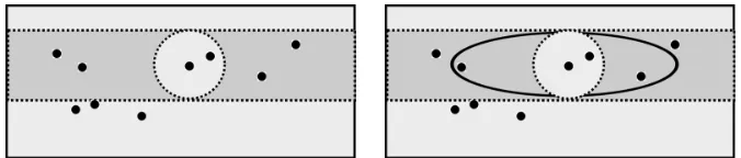
Figure 2: Balls B(x, h) before and after projection or reweighting. The dotted points are sam-ple {Xi}. Left: after projection onto 1 dimension, the new ball B(x, h) contains all
the points shown in the dotted rectangle, much more than the original ball (dotted cir-cle).Right:feature-reweighting has the approximate effect of a projection; the new ball
B(x, h)is an ellipsoid containing more points in the directions with small weight.
where the infimum is taken over all regressorsfnmapping samplesXn,Ynto anL2 measureable
function (also denotedfnfor simplicity of notation), and the expectation is taken over the draw of
ann-sample from a distribution whereE[Y|X =x] =f(x).
Thus, in a minimax sense, the best rate achievable for (non-sparse) Lipschitz functions is f the formO n−2/(2+d)
. However when the unknown function happens to beR-sparse, the better rate ofO n−2/(2+|R|)
is achievable (see e.g. Lafferty and Wasserman (2005)). The better rates are achieved for instance by performing regression on the data projected to the span ofR. This is the same as setting the weightsWi,i /∈R, to0. In other words, we would letWi be correlated with
the variation off along coordinateias discussed earlier.
To better understand why better rates are possible after a dimension reduction to the span ofR
as described above, let’s consider the case of a kernel estimatefn,h(x)using a bandwidthh. The
error offn,h(x)depends on its variance and bias. The variance itself decreases with the number of
points contributing most to the estimate: this is roughly (depending on the kernel) the number of points falling in the ballB(x, h)in the given metric space. Since balls of a fixed radius have larger mass in smaller dimensional space (illustrated in Fig. 2), projection decreases the variance of the kernel estimatefn,h(x). In addition, if the unknownf does not vary along those directionsi /∈R
eliminated by the projection, the bias of the estimatefn,h(x) remains unaffected; in other words,
the projection loses no information about the unknown f. This combined effect on variance and bias decreases the error of the estimate.
(a)SARCOS robot, joint 7. (b)Parkinson’s. (c)Telecom.
Figure 3: Typical gradient norms (estimates ofkfi0k1,µ, i∈[d]) for some real-world datasets.
2.2 Technical intuition: the non-sparse case
In this section we aim to understand how regression performance is affected by the distribution of weightsWi with respect to the variation off along coordinates. The main situation of interest is
one wherefvaries in all coordinates, but in some coordinates more than in others. This situation is captured by assuming the quantities|f0
i|supare all nonzero but some are considerably smaller than
others. We also assume that the weightsWiare nonzero for alli∈[d].
We will be bounding the error of a box-kernel regressor operating on the transformed space
(X, ρ), in terms of how the weightsWi scale relative to each other, and relative to the variation |fi0|sup. We will see that, even in non-sparse situations where all|fi0|supare far from0, it is possible to achieve finite-sample rates better than the minimax rate of Theorem 2, provided (i) the weights
Wi are sufficiently larger in scale for a small subsetR of the coordinates (for low variance), and
(ii) eachWiis sufficiently correlated with|fi0|sup(for low bias).
The results of this section uncover an interesting phenomenon, also observed in experiments, that improvement might only be possible in a specific mid-range sample size regime depending on problem parameters. This is unsurprising: when the sample size is too small, any algorithm will likely only fit noise and good rates would not be possible; as the sample size gets quite large, algorithms operating in the original space tend to also do well, and the advantage of operating in
(X, ρ)becomes negligible (see Remark below). We believe this behavior is not limited to the GW approach, because the results here are not directly tied to GW since our analysis is in terms of a general metricρof the form (1).
We will see that the attainable convergence rates are smaller than the minimax rate ofΩ(n−2/(2+d))
forngreater than some problem-specificn0 (Corollary 8). These rates tend towards the minimax
rate from below asn→ ∞.
Remark 2.1 There is theoretical intuition as to why improvement over the minimax rate is unlikely
in the asymptotic regime where n → ∞. Remember that the metric ρ is norm-induced and all
norms are equivalent on finite-dimensional spaces. In other words there existC, C0 such that for
all x, x0 ∈ Rd, Ckx−x0k ≤ ρ(x, x0) ≤ C0kx−x0k. As a consequence there exists C00 such
that, forsufficiently small, anyr-cover of aρ-ballB(x, r) centered onx ∈ X has size at least
C00−d. HereC00 depends on the metric(X, ρ). It is known (see e.g. the lower-bound of Kpotufe
(2011)) that such space covering properties influence the attainable regression rates, where larger
data sizes ncorrespond to finer coverings of the space, hence to small. We therefore postulate
only expect improvements over the minimax rate in small sample regimes, wheresmallis problem-specific. Note that this remark is of independent interest since other approaches such as metric learning would typically use norm-induced metrics.
The analysis in this section, although focusing on kernel regression, yields general intuition about the behavior of other related distance-based regressors such ask-NN, since such regressors are similarly affected by characteristics of the regression problem (e.g. smoothness off, intrinsic dimension of(X, ρ)).
We start by defining quantities which serve to describe the distribution of weightsWi.
Definition 3 For any subset of coordinatesR⊂[d], defineκR,
p
maxi∈RWi/mini∈RWi, and
let6R,2pmaxi /∈RWi. Finally we define theρ-diameterofX asρ(X),supx,x0∈Xρ(x, x0).
As discussed earlier, regression variance is small if there exists a small subset R for which the weightsWi are relatively larger than those for coordinates not inR. Formally, we want the
quanti-ties|R|,6RandκRrelatively small for someR⊂[d]. How small will become gradually clearer.
We start with two results (Lemmas 4 and 5 below) on properties of the metric space (X, ρ)
which affect the behavior of a distance-based regressor such asfn,,ρ. All omitted proofs are given
in the appendix.
The first Lemma 4 concerns the size of minimal covers (at different scales) of the metric(X, ρ). Such cover sizes influence the variance of a distance-based regressor operating on(X, ρ). If(X, ρ)
has small cover-sizes, it can typically be covered by large balls, each ball likely to contain enough data for small regression variance. Lemma 4 roughly states that, while a minimal-cover of the Euclidean spaceX ⊂Rdhas sizeO −d
, anρ(X)-cover of(X, ρ)has smaller sizeC−rwhere
|R| ≤r −−→→0 d. BothCand the functionr()depend on the relative distribution of weightsWias
captured by the quantities|R|,6RandκR.
Lemma 4 (Covering numbers) Consider R ⊂ [d]such thatmaxi /∈RWi < mini∈RWi. There
existC≤C0(4κR)|R|such that, for any >0, the smallestρ(X)-cover of(X, ρ)has size at most
C−r(), wherer()is a nondecreasing function ofsatisfying
r()≤
(
|R| if≥6R/ρ(X)
d−(d− |R|)·log(ρ(X)/6R)
log(1/) if < 6R/ρ(X)
The functionr()captures thedimensionof(X, ρ)2. We thus wantrto be small so that the transfor-mationρacts like a low-dimensional projection and hence helps reduce variance. The functionris smallest when most weights are concentrated in a small subsetR, i.e. we want small|R|and small
6R/ρ(X)(this term captures the difference in magnitude between weights not inRand weights in R). It might therefore seem preferable to chooseρ in this way, but we have to be careful: not all dimension reduction is good since such a transformation ρ might introduce additional regression bias. We therefore need to understand how regression bias is affected by the distribution of weights
Wi in the transformationρ.
Lemma 5 below captures the smoothness properties of the target functionf in the transformed metric(X, ρ). These smoothness properties affect the bias of distance-based regressors on(X, ρ).
Lemma 5 (Change in Lipschitz smoothness forf) Suppose each derivativefi0 is bounded onX
by|fi0|sup. AssumeWi >0whenever|fi0|sup > 0. Denote byRthe largest subset of[d]such that
|fi0|sup>0fori∈R. We have for allx, x0 ∈X,
f(x)−f(x0)
≤
X
i∈R |f0
i|sup
√
Wi
!
ρ(x, x0).
We want f to be as smooth as possible, in other words we want the Lipschitz parameter
P
i∈R |f0
i|sup
√
Wi
as small as possible. Suppose Wi is uncorrelated with the variation off along
i, e.g. Wi is small for those coordinates where|fi0|supis large, then the function f might end up
lacking smoothness in the modified space(X, ρ). While it is hard to estimate|fi0|sup, we can ex-pect it to be correlated withkfi0k1,µ which is easier to estimate (Section 3). Thus by keeping the weightsWi correlated with the gradient normskfi0k1,µ, we expect the functionf to remain
rela-tively smooth in the space(X, ρ)and hence we expect to maintain control on regression bias. Since it is unlikely in practice thatf varies equally in all coordinates (Figure 3), in light of Lemma 20, we will expect better regression performance in the space(X, ρ)as variance should decrease while bias remains controlled.
Remark 2.2 As previously mentioned, there are many ways to incorporate the coordinate-wise
variability of f into the weights ρ, and GW (or Relief heuristics discussed in Section 6.2) is just
one of this. In light of the Lipschitz parameter
P
i∈R |fi0|
sup
√
Wi
, we could reasonably set Wi to
approximate kfi0kq1,µ for some q > 0 (q = 1,2 in this work), or to kfi0kqi
1,µ for some power qi
depending oni. These are interesting questions deserving further investigation.
We now go further in formalizing the intuition discussed so far by considering the case of kernel regression in(X, ρ). We will derive exact conditions on the distribution of weightsWi that allow
improvements over the minimax rate ofO n−2/(2+d)in the non-asymptotic regime. The box-kernel regression estimate is defined as follows.
Definition 6 Given >0andx∈ X, the box-kernel estimate atxis defined as follows. Recall that
ρ(X),supx,x0∈Xρ(x, x0)denotes theρ-diameter ofX:
fn,,ρ(x),averageYi of pointsXi ∈B(x, ρ(X)), or0ifB(x, ρ(X))is empty.
The next lemma establishes the convergence rate for a box-kernel regressor using any given band-width ρ(X). The lemma is a simple application of known results on the bias and variance of a kernel regressor combined with the previous two lemmas on the dimension of (X, ρ) and the smoothnness off on(X, ρ).
Lemma 7 (Rate forfn,,ρ, arbitrary) Consider anyR⊂[d]such thatmaxi /∈RWi <mini∈RWi.
There exist1≤CκR ≤C
0(4κ
R)|R|, a universal constantC, andλρ≥supi|fi0|sup/
√
Wisuch that
E
Xn,Yn|fn,,ρ−f|
2≤C
κR
−r()
n +C
2d2λ2
ρ2ρ(X)2,
Proof By Lemma 5,f is (dλρ)-Lipschitz on(X, ρ). We can then apply Theorem 5.2 of Gyorfi
et al. (2002)3to bound theL2 error as
E
Xn,YnEX|fn,,ρ(X)−f(X)|
2 ≤C2
1
N n +C
2d2λ2
ρ2ρ(X)2,
for some universal constantsC1, C, whereNdenotes the size of a minimalρ(X)-cover of(X, ρ).
Apply Lemma 4 to conclude.
We can now derive conditions on the distribution of weights (X, ρ) that permit good perfor-mance relative to the minimax rate ofO n−2/(2+d). These conditions are given in equation (2). The main message of Corollary 8 below is that improvement in rate is possible in the non-asymptotic regime under rather mild conditions on the distribution of weightsWi, even though improvement
might not be possible in the asymptotic regime. In light of (2) sparseness (as described in Section 2.1) is not required, we simply need the functionfto vary more along a small subset of coordinates (R ⊂[d]) than along other coordinates, provided the weightsWi are properly correlated with the
variation inf along coordinates. The correlation betweenWiand gradients off is implicit in the
ratioλρρ(X)/λof (2). The quantity λcaptures the smoothness of f before the data
transforma-tionρ, whileλρcaptures the smoothness off after the transformationρ. The ratioλρρ(X)/λthus
captures the loss in smoothness (taking into account the change in diameter from1 toρ(X)) due to the transformation ρ, and this loss is controlled if Wi is correlated with the magnitude of the
coordinate-wise derivatives off.
Corollary 8 (Rate forfn,,ρ, optimal) Letλ,supi∈[d]|fi0|supandλρ ,supi∈[d]|fi0|sup/
√
Wi.
Note that by definitionf ∈ Fλ. LetCκR andC be defined as in Lemma 7, and˜cas in Theorem 2.
Suppose the following holds for someR⊂[d]:
(d− |R|) log
ρ(X
) 6R
≥dlog
Cλρρ(X) λ
+ log
CκR
˜ c
. (2)
Then there existsn0 for which the following holds. For alln≥n0, there exist a bandwidthn, and
r=r(n), where|R| ≤r < d, such that,
Ekfn,n,ρ−fk
2≤2C2/2+r
κR (Cdλρρ(X))
2r/(2+r)n−2/2+r<inf
fn
sup Fλ
Ekfn−fk2.
Proof For >0, andn∈N. Letr()as in Lemma 4. Define the functionsψn,ρ() =CκR
−r()/n,
andψn,6ρ() =C10−d/n, whereC10 = ˜c(λ/Cλρρ(X))d. We also defineφ() =C2d2λ2ρρ(X)2·2.
Now recall (Theorem 2) that the minimax rate can be bounded below by
2˜c2/(2+d)(dλ)2d/(2+d)n−2/2+d.
For any fixedn, letn,6ρbe a solution toψn,6ρ() =φ(). Solving forn,6ρ, we see that the minimax
rate is bounded below by
2φ(n,6ρ) = 2˜c2/(2+d)(dλ)2d/(2+d)n−2/2+d.
For anyn∈ N, there exists a solutionn,ρto the equationψn,ρ() = φ()sincer()is
nonde-creasing. Therefore, by Lemma 7, we have
E
Xn,Ynkfn,,ρ−fk
2 ≤2φ(
n,ρ).
We therefore want to show for a certain range ofn∈ Nthatφ(n,ρ) < φ(n,6ρ), equivalently that n,ρ < n,6ρ. First notice that, since φ is independent of n, and bothψn,ρ and ψn,6ρ are strictly
decreasing functions ofn, we have thatn,ρandn,6ρboth tend to0asn→ ∞. Therefore we can
definen0such that, for alln≥n0, bothn,ρandn,6ρare less than6R/ρ(X).
Thus,∀n ≥n0, we haven,ρ < n,6ρif, for all0 < < 6R/ρ(X),ψn,ρ() < ψn,6ρ(). This is
insured by the conditions of equation (2), which are derived by recalling the bound of Lemma 4 on
r()for the range0< < 6R/ρ(X).
2.3 The Case of Classification
We continue the intuition developed in the last section about the GW method with the case of classification, more preciselyplug-inclassification, defined as follows. LetY ∈ {0,1}, and letηn
denote an estimate of the error functionη(x),E[Y|x] =P(Y = 1|x). Then1{ηn(x)>1/2}is
a plug-in classification rule, emulating the Bayes optimal-classification rule1{η(x)>1/2}. Two common examples of plug-in classification rules are the k-NN classifier and the -NN classifier which estimateY atxas the majority label amongst, respectively, theknearest neighbors ofx, and the neighbors within distanceofx. For both methods, the implicit estimateηnofηis the
averageY value of the neighbors ofx.
The GW method for classification naturally corresponds to estimating the gradient normskηi0k1,µ
of the directional derivativesηi0.
Since ηn is actually a regression estimate of the function η(x), the0-1classification error of
plug-in methods is related to that of regression as shown in the following well-known result.
Lemma 9 (Devroye et al. (1996)) Letηn(x)be an estimator ofη(x), and let err(η), err(ηn),
de-note respectively the classification error rates of the Bayes classifier and that of the plug-in
classi-fication rule1{ηn(x)>1/2}. We have
err(ηn)−err(η)≤2E
X|ηn(X)−η(X)|.
A bound on the classification error of-NN (operating in(X, ρ)) easily follows from Lemma 9 above and the analysis of the previous section on the properties of the space(X, ρ).
Lemma 10 Defineηn,,ρ(x)as the averageY value of the points inXn∩Bρ(x, ρ(X))for some > 0. Let r() be defined as in Corollary 4. There exist a constant1 ≤CκR ≤ C
0(4κ
R)|R|/2, a
universal constantC, and a constantλρ≥supi|η0i|sup/
√
Wisuch that
E
Xn,Yn|err(ηn,,ρ)−err(η)| ≤CκR
r
−r()
Proof Using Lemma 9 and applying Jensen’s inequality twice, we have
E
Xn,Yn|err(ηn,,ρ)−err(η)| ≤
r
E
Xn,YnEX|ηn,,ρ(X)−η(X)|
2
.
Thus, we just need to bound theL2error ofηn,,ρ, which is a kernel regressor with a box kernel of
bandwidthρ(X). Apply Lemma 7 and conclude.
It follows similarly as in the case of regression that it is possible to achieve faster rates than the minimax rates even when the regression functionηis not sparse, providedηdoes not vary equally in all coordinates. The exact conditions are exactly those of equation (2) with the constantsCκRand
Cof Lemma 10 above (this is easily derived from the above lemma as it was done for regression).
3. Estimating the GWWi
In all that follows we are givenn i.i.d samples(Xn,Yn) = {(Xi, Yi)}ni=1 from some unknown
distribution with marginalµ. The marginalµhas supportX ⊂Rdwhile the outputY ∈
R.
The kernel estimate atxis defined using any kernelK(u), positive on[0,1/2], and0foru >1. IfB(x, h)∩Xn=∅,fn,h(x) =EnY, otherwise
fn,ρ,h¯ (x) =
n
X
i=1
K( ¯ρ(x, Xi)/h)
Pn
j=1K( ¯ρ(x, Xj)/h) ·Yi=
n
X
i=1
wi(x)Yi, (3)
for some metricρ¯and a bandwidth parameterh.
For the kernel regressor fn,h used to learn the metricρ below, ρ¯is the Euclidean metric. In
the analysis we assume the bandwidth forfn,his set ash ≥ log2(n/δ)/n
1/d
, given a confidence parameter0< δ <1. In practice we would learnhby cross-validation, but for the analysis we only need to know the existence of a good setting ofh.
We estimate the normkfi0k1,µas follows:
∇n,i,En
|fn,h(X+tei)−fn,h(X−tei)|
2t ·1{An,i(X)}=En[∆t,ifn,h(X)·1{An,i(X)}],
(4)
whereAn,i(X) is the event that enoughsamples contribute to the estimate∆t,ifn,h(X). For the
consistency result, we assume the following setting:
An,i(X)≡ min
s∈{−t,t}µn(B(X+sei, h/2))≥αnwhereαn,
2dln 2n+ ln(4/δ)
n .
The metricρis then obtained by setting the weightsWi to either∇n,ior the squared estimate ∇2
n,iin all our experiments.
4. Consistency of the estimatorWiofkfi0k1,µ
4.1 Theoretical setup
4.1.1 MARGINALµ
This is for instance the case if µhas a lower-bounded density onX. Under this assumption, for samplesXin dense regions,X±tei is also likely to be in a dense region.
4.1.2 REGRESSION FUNCTION AND NOISE
The outputY ∈ Ris given asY =f(X) +η(X), whereEη(X) = 0. We assume the following
general noise model:∀δ >0there existsc >0such that supx∈XPY|X=x(|η(x)|> c)≤δ.
We denote byCY(δ)the infimum over all suchc. For instance, supposeη(X)has exponentially
decreasing tail, then∀δ >0,CY(δ)≤O(ln 1/δ). A last assumption on the noise is that the variance
of(Y|X=x)is upper-bounded by a constantσ2Y uniformly over allx∈ X.
Define theτ-envelopeofXasX+B(0, τ),{z∈B(x, τ), x∈ X }. We assume there existsτ
such thatfis continuously differentiable on theτ-envelopeX+B(0, τ). Furthermore, each deriva-tivefi0(x) =e>i ∇f(x)is upper bounded onX+B(0, τ)by|fi0|supand is uniformly continuous on
X +B(0, τ)(this is automatically the case if the supportX is compact).
4.1.3 DISTRIBUTIONAL PARAMETERS
Our consistency results are expressed in terms of the following distributional quantities. Fori∈[d], define the(t, i)-boundaryofX as∂t,i(X) , {x:{x+tei, x−tei} 6⊂ X }. The smaller the mass µ(∂t,i(X))at the boundary, the better we approximatekfi0k1,µ.
The second type of quantity ist,i ,supx∈X, s∈[−t,t]|fi0(x)−fi0(x+sei)|.
Since µhas continuous density on X and ∇f is uniformly continuous on X +B(0, τ), we automatically haveµ(∂t,i(X))
t→0
−−→0andt,i t→0
−−→0.
4.2 Main theorem
Our main theorem bounds the error in estimating each normkfi0k1,µwith∇n,i. The main technical
hurdles are in handling the various sample inter-dependencies introduced by both the estimates
fn,h(X)and the eventsAn,i(X), and in analyzing the estimates at the boundary ofX.
Theorem 11 Lett+h≤τ, and let0< δ <1. There existC =C(µ, K(·))andN =N(µ)such
that the following holds with probability at least1−2δ. DefineA(n),Cd·log(n/δ)·CY2(δ/2n)·
σY2/log2(n/δ). Letn≥N, we have for alli∈[d]:
∇n,i−
fi0
1,µ
≤
1 t
r
A(n) nhd +h·
X
i∈[d] fi0
sup
+ 2
fi0
sup r
ln 2d/δ
n +µ(∂t,i(X))
!
+t,i.
The bound suggests to set t in the order of h or larger. We need t to be small in order for
µ(∂t,i(X))andt,ito be small, buttneeds to be sufficiently large (relative toh) for the estimates fn,h(X+tei)andfn,h(X−tei)to differ sufficiently so as to capture the variation inf alongei.
The theorem immediately implies consistency for t −−−→n→∞ 0, h −−−→n→∞ 0,h/t −−−→n→∞ 0, and
(n/logn)hdt2−−−→ ∞n→∞ . This is satisfied for many settings, for examplet∝√handh∝1/logn.
4.3 Proof of Theorem 11
The main difficulty in bounding
∇n,i− kf
0 ik1,µ
results from certain dependencies between random
inXn, and thus introduce inter-dependencies between the estimates∆t,ifn,h(X)for different points Xin the sampleXn.
To handle these dependencies, we carefully decompose
∇n,i− kf
0 ik1,µ
,i∈[d], starting with:
∇n,i−
fi0
1,µ ≤
∇n,i−En
fi0(X)
+ En
fi0(X)
−
fi0
1,µ . (5)
The following simple lemma bounds the second term of (5).
Lemma 12 With probability at least1−δ, we have for alli∈[d],
En
fi0(X)
−
fi0
1,µ ≤ fi0
sup· r ln 2d/δ n .
Proof Apply a Chernoff bound, and a union bound oni∈[d].
Now the first term of equation (5) can be further bounded as
∇n,i−En
fi0(X)
≤
∇n,i−En
fi0(X)
·1{An,i(X)}
+En
fi0(X)
·1
¯
An,i(X) ≤
∇n,i−En
fi0(X)
·1{An,i(X)}
+
fi0
sup·En1
¯
An,i(X) . (6)
We will bound each term of (6) separately.
The next lemma bounds the second term of (6). It is proved in the appendix. The main tech-nicality in this lemma is that, for any X in the sample Xn, the event A¯n,i(X) depends on other
samples inXn.
Lemma 13 Let∂t,i(X)be defined as in Section (4.1.3). For n ≥ n(µ), with probability at least
1−2δ, we have for alli∈[d],
En1
¯
An,i(X) ≤
r
ln 2d/δ
n +µ(∂t,i(X)).
It remains to bound |∇n,i−En|fi0(X)| ·1{An,i(X)}|. To this end we need to bring in f
through the following quantities:
e
∇n,i,En
|f(X
+tei)−f(X−tei)|
2t ·1{An,i(X)}
=En[∆t,if(X)·1{An,i(X)}]
and for anyx∈ X, definef˜n,h(x),EYn|Xnfn,h(x) =Piwi(x)f(xi).
The quantity∇en,iis easily related toEn|fi0(X)|·1{An,i(X)}. This is done in Lemma 14 below.
The quantityf˜n,h(x)is needed when relating∇n,ito∇en,i.
Lemma 14 Definet,ias in Section (4.1.3). With probability at least1−δ, we have for alli∈[d],
∇en,i−En
fi0(X)
·1{An,i(X)}
Proof We havef(x+tei)−f(x−tei) =
Rt
−tf 0
i(x+sei)dsand therefore
2t fi0(x)−t,i
≤f(x+tei)−f(x−tei)≤2t fi0(x) +t,i
.
It follows that21t|f(x+tei)−f(x−tei)| − |fi0(x)|
≤t,i, therefore
∇en,i−En
fi0(X)
·1{An,i(X)}
≤En
1
2t|f(x+tei)−f(x−tei)| −
fi0(x)
≤t,i.
It remains to relateWito∇en,i. We have
2t
∇n,i−∇en,i
=2t|En(∆t,ifn,h(X)−∆t,if(X))·1{An,i(X)}|
≤2 max
s∈{−t,t}En|fn,h(X+sei)−f(X+sei)| ·1{An,i(X)}
≤2 max s∈{−t,t}En
fn,h(X+sei)−
˜
fn,h(X+sei)
·1{An,i(X)} (7)
+ 2 max s∈{−t,t}En
˜
fn,h(X+sei)−f(X+sei)
·1{An,i(X)}. (8)
We first handle the bias term (8) in the next lemma which is given in the appendix.
Lemma 15 (Bias) Lett+h≤τ. We have for alli∈[d], and alls∈ {t,−t}:
En
˜
fn,h(X+sei)−f(X+sei)
·1{An,i(X)} ≤h· X
i∈[d] fi0
sup.
The variance term in (7) is handled in the lemma below. The proof is given in the appendix.
Lemma 16 (Variance terms) There existC =C(µ, K(·))such that, with probability at least1−
2δ, we have for alli∈[d], and alls∈ {−t, t}:
En
fn,h(X+sei)−
˜
fn,h(X+sei)
·1{An,i(X)} ≤ s
Cd·log(n/δ)C2
Y(δ/2n)·σ2Y
n(h/2)d .
The next lemma summarizes the above results:
Lemma 17 Lett+h≤τ and let0 < δ <1. There existC =C(µ, K(·))such that the following
holds with probability at least1−2δ. DefineA(n),Cd·log(n/δ)·CY2(δ/2n)·σY2/log2(n/δ).
We have
∇n,i−En
fi0(X)
·1{An,i(X)}
≤ 1 t r A(n) nhd +h·
X
i∈[d] fi0
sup
+t,i.
Proof Apply lemmas 14, 15 and 16, in combination with equations 7 and 8.
5. Experimental Evaluation of the GW Approach
We have so far derived GW based on the theoretical principles of Section 2, namely that perfor-mance improvements are possible if data coordinates are weighted according to the coordinate-wise variation of the unknownf, and iff varies unevenly across coordinates. In this section, we verify these theoretical principles empirically on various real-world datasets. The code and all the data sets used in these experiments are publicly available athttp://goo.gl/bCfS78
We consider kernel,k-NN and SVM (support vector) approaches on a variety of controlled (ar-tificial) and real-world datasets. We emphasize that our goal is to demonstrate the benefits of GW in improving the performance of these successful and popular procedures on a wide range of datasets. We do not aim to beat results that may have been obtained on these data using procedures other than kernel,k-NN and SVM approaches, since this is not required for a practical validation of our theoretical results. We also note that, throughout the experiments, we only retain the numerical at-tributes in each data set, and discard all the categorical atat-tributes. Therefore, our reported prediction errors on some datasets might differ from others reported in the literature at large.
Parameter settings and general comments: Recall that, for the GW approach, we might set the componentsWi of the metricρto∇qn,i. The exponentq (cf. Remark 2.2) is a parameter left
open by our theoretical analysis. In our experiments, we explore the choicesq = 1, as in Kpotufe and Boularias (2012), andq = 2which serves to further emphasize the difference in importance between coordinates.
The resulting performance of the GW approach depends on the parameters used to learn∇n,i,
En[∆t,ifn,h(X)·1{An,i(X)}]. These are the bandwidthh used in the estimatefn,h(X)and the
parametertin∆t,ifn,h(X),|fn,h(X+tei)−fn,h(X−tei)|/2t. In the majority of experiments
(reported in the main body of the paper) we tuneh, but we don’t tunet and simply sett = h/2
as a rule of thumb. This results in faster training time, and although not optimal, still results in significant performance gains for the various regression and classification procedures where GW is used to preprocess the data. If in addition we properly tunet, the observed performance gains are even more significant as reported in Tables 4 and 5 of the Appendix.
We emphasize that the GW approach is computationally cheap: it only adds to training time since it only involves pre-processing the data. No significant difference is observed in estimation time, i.e. in computing regression or classification estimates using the preprocessed data vs using the original data. In fact estimation time can even be smaller after preprocessing since GW can act as an approximate dimension-reduction given the sparsity in the data. The average prediction times are reported in Table 6 of the appendix.
Our experiments are divided as follows. First we show the attainable performance gains by using GW for regression, then we show that GW works well also for classification. At the end of the section we explore the tradeoffs between feature selection and feature weigthing.
5.1 Regression experiments
5.1.1 DATA DESCRIPTION
The first two data sets describe the dynamics of7degrees of freedom of robotic arms, Barrett WAM and SARCOS (Nguyen-Tuong et al., 2009; Nguyen-Tuong and Peters, 2011). The input points are
21-dimensional and correspond to samples of the positions, velocities, and accelerations of the 7
joints. The output points correspond to the torque of each joint. The far joints (1, 5, 7) correspond to different regression problems and are the only results reported. As expected, results for other joints were found to be similarly good.
Another data set describes the probabilities of achieving successful grasping actions performed by a robot on different piles of objects (Boularias et al., 2014a,b). Each data point describes one grasping action performed at a particular location on the surface of a pile of objects. The objects are mostly rocks and rubble with unknown and irregular shapes. An input point is a150-dimensional vector and corresponds to a patch of a depth image obtained by projecting the robotic hand on the scene. The output is a value between0and1.
The other data sets are taken from the UCI repository (Frank and Asuncion, 2012) and from (Torgo, 2012). The concrete strength data set (Concrete Strength) contains8-dimensional input points, de-scribing age and ingredients of concrete, the output points are the compressive strength. The wine quality data set (Wine Quality) contains11-dimensional input points corresponding to the physico-chemistry of wine samples, the output points are the wine quality. The ailerons data set (Ailerons) is taken from the problem of flying a F16 aircraft. The 5-dimensional input points describe the status of the aeroplane, while the goal is to predict the control action on the ailerons of the aircraft. The housing data set (Housing) concerns the task of predicting housing values in areas of Boston, the input points are13-dimensional. The Parkinson’s Telemonitoring data set (Parkison’s) is used to predict the clinician’s Parkinson’s disease symptom score using biomedical voice measurements represented by21-dimensional input points. We also consider a telecommunication problem (Tele-com), wherein the47-dimensional input points and the output points describe the bandwidth usage in a network.
5.1.2 EXPERIMENTAL SETUP
For all data sets, we normalize each coordinate with its standard deviation from the training data. To learn the metric, we set hby cross-validation on half the training points, and we sett = h/2
for all data sets. Note that in practice we might want to also tune t in the range of h for even better performance than reported here. The event An,i(X) is set to reject the gradient estimate ∆n,ifn,h(X)atXif no sample contributed to one of the estimatesfn,h(X±tei).
In each experiment, we compare kernel regression in the Euclidean metric space (KR) and in the learned metric space with gradient weights (KR-ρ) and with squared gradient weights (KR-ρ2),
where we use a box kernel for the three methods. Similar comparisons are made usingk-NN,k
-NN-ρandk-NN-ρ2. All methods are implemented using a fast neighborhood search procedure, namely the cover-tree of (Beygelzimer et al., 2006), and we also report in the supplementary material the average prediction times so as to confirm that, on average, time-performance is not affected by using the metric.
The parameter k in k-NN, k-NN-ρ, k-NN-ρ2, and the bandwidth in KR, KR-ρ, KR-ρ2 are learned by cross-validation on half of the training points. We try the same range ofk(from 1to
is done efficiently by starting with a log search to quickly reduce the search space, followed by a grid search on the resulting smaller range.
Table 1 shows the normalized Mean Square Errors (nMSE) where the MSE on the test set is normalized by variance of the test output. We use1000 training points in the robotic, Telecom, Parkinson’s, and Ailerons data sets, and 2000 training points in Wine Quality, 730 in Concrete Strength, and300in Housing. We used2000test points in all of the problems, except for Concrete,
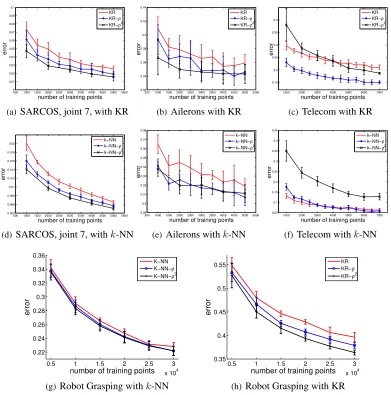
300points, Housing, 200points, and Robot Grasping, 10000points. Averages over 10 random experiments are reported. For the larger data sets (SARCOS, Ailerons, Telecom, Grasping) we also report the behavior of the algorithms, with and without metric, as the training sizenincreases (Figure 4).
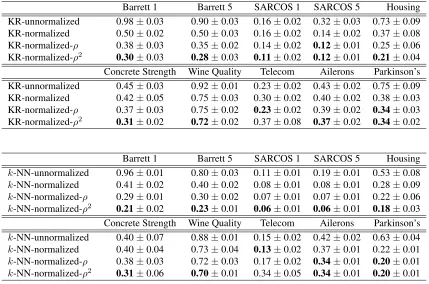
Barrett 1 Barrett 5 SARCOS 1 SARCOS 5 Housing KR-unnormalized 0.98±0.03 0.90±0.03 0.16±0.02 0.32±0.03 0.73±0.09 KR-normalized 0.50±0.02 0.50±0.03 0.16±0.02 0.14±0.02 0.37±0.08 KR-normalized-ρ 0.38±0.03 0.35±0.02 0.14±0.02 0.12±0.01 0.25±0.06 KR-normalized-ρ2 0.30±0.03 0.28±0.03 0.11±0.02 0.12±0.01 0.21±0.04 Concrete Strength Wine Quality Telecom Ailerons Parkinson’s KR-unnormalized 0.45±0.03 0.92±0.01 0.23±0.02 0.43±0.02 0.75±0.09 KR-normalized 0.42±0.05 0.75±0.03 0.30±0.02 0.40±0.02 0.38±0.03 KR-normalized-ρ 0.37±0.03 0.75±0.02 0.23±0.02 0.39±0.02 0.34±0.03 KR-normalized-ρ2 0.31±0.02 0.72±0.02 0.37±0.08 0.37±0.02 0.34±0.02
Barrett 1 Barrett 5 SARCOS 1 SARCOS 5 Housing
k-NN-unnormalized 0.96±0.01 0.80±0.03 0.11±0.01 0.19±0.01 0.53±0.08
k-NN-normalized 0.41±0.02 0.40±0.02 0.08±0.01 0.08±0.01 0.28±0.09
k-NN-normalized-ρ 0.29±0.01 0.30±0.02 0.07±0.01 0.07±0.01 0.22±0.06
k-NN-normalized-ρ2 0.21±0.02 0.23±0.01 0.06±0.01 0.06±0.01 0.18±0.03 Concrete Strength Wine Quality Telecom Ailerons Parkinson’s
k-NN-unnormalized 0.40±0.07 0.88±0.01 0.15±0.02 0.42±0.02 0.63±0.04
k-NN-normalized 0.40±0.04 0.73±0.04 0.13±0.02 0.37±0.01 0.22±0.01
k-NN-normalized-ρ 0.38±0.03 0.72±0.03 0.17±0.02 0.34±0.01 0.20±0.01
k-NN-normalized-ρ2 0.31±0.06 0.70±0.01 0.34±0.05 0.34±0.01 0.20±0.01
Table 1: Normalized mean square prediction errors show that, in almost all cases, gradient weights improve accuracy in practice. The top three tables are for KR vs KR-ρand KR-ρ2, the bot-tom three fork-NN vsk-NN-ρandk-NN-ρ2.k-NN-unnormalized and KR-unnormalized
refer tok-NN and KR used on unnormalized data. For all the other methods, data vectors are normalized by dividing each data vector by the standard deviation of the training data in each dimension.
5.1.3 DISCUSSION OF RESULTS
500 1000 1500 2000 2500 3000 3500 4000 4500 5000 5500 0 0.01 0.02 0.03 0.04 0.05 0.06 0.07 0.08 0.09 0.1
number of training points
error
KR KR−ρ KR−ρ2
(a) SARCOS, joint 7, with KR
500 1000 1500 2000 2500 3000 3500 4000 4500 5000 5500 0.32 0.34 0.36 0.38 0.4 0.42 0.44
number of training points
error
KR KR−ρ
KR−ρ2
(b)Ailerons with KR
1000 2000 3000 4000 5000 6000 7000
0.15 0.2 0.25 0.3 0.35 0.4
number of training points
error
KR KR−ρ KR−ρ2
(c)Telecom with KR
500 1000 1500 2000 2500 3000 3500 4000 4500 5000 5500 0.004 0.006 0.008 0.01 0.012 0.014 0.016 0.018 0.02
number of training points
error
k−NN k−NN−ρ k−NN−ρ2
(d)SARCOS, joint 7, withk-NN
500 1000 1500 2000 2500 3000 3500 4000 4500 5000 5500 0.29 0.3 0.31 0.32 0.33 0.34 0.35 0.36 0.37 0.38
number of training points
error
k−NN k−NN−ρ k−NN−ρ2
(e)Ailerons withk-NN
1000 2000 3000 4000 5000 6000 7000 0.05 0.1 0.15 0.2 0.25 0.3 0.35 0.4 0.45
number of training points
error
k−NN k−NN−ρ k−NN−ρ2
(f) Telecom withk-NN
0.5 1 1.5 2 2.5 3
x 104 0.22 0.24 0.26 0.28 0.3 0.32 0.34 0.36
number of training points
error
K−NN K−NN−ρ K−NN−ρ2
(g)Robot Grasping withk-NN
0.5 1 1.5 2 2.5 3
x 104 0.35
0.4 0.45 0.5 0.55
number of training points
error
KR
KR−ρ
KR−ρ2
(h)Robot Grasping with KR
Figure 4: Plotting regression error as a function of the number of training points shows that gradient weights lead to a clear improvement even for small sample sizes, indicating that our estimator ofkfi0k1,µproduces useful results even from relatively few samples.
that the Telecom data set has a lot of outliers and this probably explains the discrepancy, besides the fact that we did not attempt to tunet(see Trivedi et al. (2014) for experiments wheretis additionally tuned, and where GW clearly outperforms the baselines for the Telecom dataset).
Also notice that the error ofk-NN is already low for small sample sizes, making it harder to outperform. However, as shown in Figure 4, for larger training sizesk-NN-ρ gains onk-NN. We also note that methods using squared gradient weights (k-NN-ρ2 and KR-ρ2) achieved a better performance compared to other methods. The only exception here is also Telecom, where the non-squared gradient weights yield a lower prediction error. The rest of the results in Figure 4 where we varynare self-descriptive: gradient weighting clearly improves the performance of the distance-based regressors.
Finally, we note that the average prediction times (reported in the supplementary material) is nearly the same for all the methods. Last, remember that the metric can be learned online at the cost of only2dtimes the average kernel estimation time reported.
5.2 Classification experiments
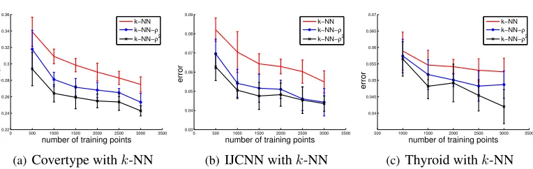
5.2.1 DATA DESCRIPTION
We tested the gradient weights method on six different data sets taken from the UCI repository (Frank and Asuncion, 2012) and from the LIBSVM website (Fan, 2012). Thecovertypedata set contains predictions of binary forest cover types from cartographic features given by 10 real variables among 54 other variables. This data set originally consists of seven different cover types, but only the two largest categories are selected for binary classification. TheMAGIC gammadata set consists of 10 features and predicts the registration of high energy gamma particles in a ground-based atmospheric Cherenkov gamma telescope. TheIJCNNdata set contains predictions of one binary output from four different time series, described by 10 categorical variables and 12 real variables. Theshuttle
data set contains 9 numerical attributes. The original data set has seven different categories, but for binary classification we merged all the classes into one class, except the first class which corre-sponds to approximately 80% of all the data. Thepage blocksdata set predicts whether a block in a given document is a text block using 10 real-valued features. We also consider thethyroid
data set where the problem is to determine whether a given patient is hypothyroid. There are three different output classes in this data set, the condition of a patient is described by 6 real variables and 15 categorical variables.
5.2.2 EXPERIMENTAL SETUP
The setup for the classification experiments is similar to the one used in the regression experiments. For all data sets, we normalize each coordinate with its standard deviation from the training data. We use the training data to compute the gradient weights. Parameter t is set proportionally to the difference between the minimum and the maximum values of each feature to account for the differences between features scales that remain after normalization. One can also consider using the learned gradient weights to sett and to re-estimate the gradient weights again, in a repeated iterative process. The probabilityP(Ci|x)of each classCi, used for calculating the feature weights,
is estimated by weightedk-NN with Gaussian kernel.
0 500 1000 1500 2000 2500 3000 3500 0.22
0.24 0.26 0.28 0.3 0.32 0.34 0.36
number of training points
error
k−NN k−NN−ρ k−NN−ρ2
(a) Covertype withk-NN
0 500 1000 1500 2000 2500 3000 3500 0.03
0.04 0.05 0.06 0.07 0.08 0.09
number of training points
error
k−NN k−NN−ρ k−NN−ρ2
(b)IJCNN withk-NN
500 1000 1500 2000 2500 3000 3500 0.04
0.045 0.05 0.055 0.06 0.065 0.07
number of training points
error
k−NN k−NN−ρ k−NN−ρ2
(c)Thyroid withk-NN
Figure 5: As in the regression case, classification benefits from gradient weights even if they were estimated from relatively few samples.
Covertype IJCNN MAGIC Gamma Shuttle Page Blocks
k-NN error 0.29±0.01 0.0629±0.0038 0.1884±0.0118 0.0031±0.0011 0.0346±0.0044
k-NN-ρerror 0.27±0.01 0.0510±0.0047 0.1858±0.0086 0.0019±0.0010 0.0338±0.0052
k-NN-ρ2error 0.25±0.01 0.0482±0.0060 0.1875±0.0092 0.0019±0.0008 0.0337±0.0046
e-NN error 0.28±0.01 0.0841±0.0061 0.1773±0.0080 0.0126±0.0026 0.0450±0.0035
e-NN-ρerror 0.26±0.01 0.0716±0.0059 0.1741±0.0069 0.0109±0.0028 0.0427±0.0031
e-NN-ρ2error 0.25±0.01 0.0651±0.0041 0.1721±0.0073 0.0093±0.0020 0.0404±0.0032
Table 2: Error rates with and without gradient weights show that they improve classification accu-racy, especially when they are used in their squared form. This is true for two different distance-based classifiers,k-NN (top), and-NN (bottom).
followed by a linear search in a smaller interval. All classification experiments are performed using
2000points for testing and up to3000points for learning. Averages over10random experiments are reported. The purpose of varying the size of training data is to report the performance as a func-tion of the number of training points (Figure 5). Table 2 shows the classificafunc-tion error rates of the different methods.
5.2.3 DISCUSSION OF RESULTS
From the results in Table 2, we see that the gradient weights metric improves the performance of the two different distance-based classifiers,k-NN and-NN. We also notice that the squared gradient weights perform better than the non-squared weights in almost all cases. The only exception is the MAGIC Gamma data set where the performance of the different classifiers seems unaffected by the choice of the metric. This is due to the fact that the gradient weights in this particular problem are nearly the same for every feature, as shown in the appendix.
0 2 4 6 8 10 12 14 16 18 20 22 0 0.1 0.2 0.3 0.4 0.5 0.6 0.7 0.8
number of selected features
error
KR with feature selection
KR−ρ
KR−ρ2
(a) Barrett, joint 1
0 2 4 6 8 10 12 14 16 18 20 22 0 0.1 0.2 0.3 0.4 0.5 0.6 0.7 0.8
number of selected features
error
KR with feature selection
KR−ρ
KR−ρ2
(b)Barrett, joint 5
0 2 4 6 8 10 12 14 16 18 20 22
0.1 0.15 0.2 0.25 0.3 0.35 0.4
number of selected features
error
KR with feature selection KR−ρ
KR−ρ2
(c) Sarcos, joint 1
0 2 4 6 8 10 12 14 16 18 20 22
0.1 0.15 0.2 0.25 0.3 0.35 0.4 0.45 0.5 0.55 0.6
number of selected features
error
KR with feature selection KR−ρ
KR−ρ2
(d)Sarcos, joint 5
0 2 4 6 8 10 12 14
0.1 0.2 0.3 0.4 0.5 0.6 0.7 0.8
number of selected features
error
KR with feature selection
KR−ρ
KR−ρ2
(e)Housing
0 1 2 3 4 5 6 7 8 9
0.3 0.4 0.5 0.6 0.7 0.8 0.9
number of selected features
error
KR with feature selection
KR−ρ
KR−ρ2
(f) Concrete Strength
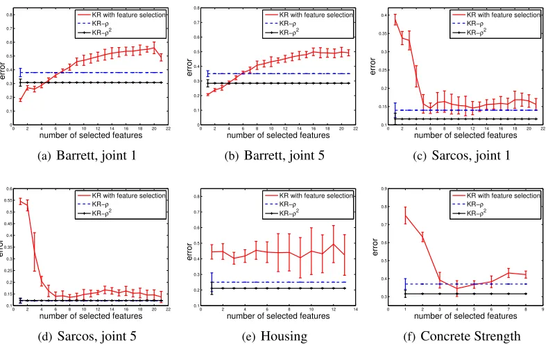
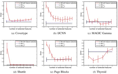
Figure 6: Kernel regression with feature selection, versus GW. On these datasets, feature weighting tends to outperform feature selection, especially when all features happen to be relevant.
regime depending on the problem, so the same behavior (as for the other data sets) is likely for the Thyroid case if we had larger samples to work with.
5.3 Feature selection vs feature weighting
How does feature weighting compare with feature selection? Feature weighting, as done with GW, has the obvious advantage of avoiding the combinatorial problem of having to select a subset of features, and gets rid of the ill-defined problem of selecting a goodimportance thresholdfor feature selection. Another less obvious advantage of feature weighting is that we do not lose much in per-formance if it so happens that all features are relevant, since weighting uses all features. However, feature selection reduces dimension and therefore variance, and would be expected to be the better option if some features are much more important than all others (i.e.f is nearly sparse); how much do we lose by feature weighting in this sort of situation, i.e. does the computational advantage of weighting justify its use? This of course depends on problem-specific costs, but we will attempt here to better understand the differences between the two approaches.
0 2 4 6 8 10 12 0.2 0.25 0.3 0.35 0.4 0.45 0.5
number of selected features
Error
k−NN with feature selection
k−NN−ρ
k−NN−ρ2
(a) Covertype
0 2 4 6 8 10 12 14
0.04 0.05 0.06 0.07 0.08 0.09 0.1 0.11
number of selected features
Error
k−NN with feature selection
k−NN−ρ
k−NN−ρ2
(b)IJCNN
0 2 4 6 8 10 12
0.16 0.18 0.2 0.22 0.24 0.26 0.28 0.3
number of selected features
Error
k−NN with feature selection k−NN−ρ
k−NN−ρ2
(c) MAGIC Gamma
0 1 2 3 4 5 6 7 8 9 10
0 0.02 0.04 0.06 0.08 0.1 0.12 0.14
number of selected features
Error
k−NN with feature selection k−NN−ρ
k−NN−ρ2
(d)Shuttle
0 2 4 6 8 10 12
0.02 0.03 0.04 0.05 0.06 0.07 0.08
number of selected features
Error
k−NN with feature selection k−NN−ρ
k−NN−ρ2
(e)Page Blocks
0 1 2 3 4 5 6 7
0.025 0.03 0.035 0.04 0.045 0.05 0.055 0.06 0.065 0.07
number of selected features
Error
k−NN with feature selection
k−NN−ρ
k−NN−ρ2
(f) Thyroid
Figure 7: Experiments onk-NN classification with feature selection versus GW. Again, GW gen-erally performs better, while little is lost when feature selection is preferable.
comparing combinations of features is to use some kind of thresholding, but as mentioned earlier, it is often unclear how to properly threshold feature importance.
Figure 6 shows that overall GW with kernel regression is competitive with the more expensive feature selection, and even often achieves better performance in those situations where all features happen to be relevant (Sarcos, Housing, Concrete). Similar results are achieved fork-NN regression, and are reported in the supplementary material.
Notice that, in those cases where feature selection performs best (Barret datasets), its gain over GW is smallest when we used the squared version∇2
n,iof GW (denoted KR-ρ2in the figure). This
is because squaring emphasizes the differences in variability offbetween features and is thus closer to feature selection.
Figure 7 repeats the same experiments in the case of classification withk-NN. Here the perfor-mance of feature selection depends more crucially on the number of selected features, and can be bad in most cases if too few features are selected. GW outperforms feature selection in most cases but the Thyroid dataset. However, even in the Thyroid case, the advantage is small, less than 2%.
0 500 1000 1500 2000 2500 3000 3500 0.22
0.24 0.26 0.28 0.3 0.32 0.34
number of training points
error
SVM SVM−ρ SVM−ρ2
(a)Covertype with SVM
0 500 1000 1500 2000 2500 3000 3500
0.04 0.05 0.06 0.07 0.08 0.09 0.1
number of training points
error
SVM SVM−ρ SVM−ρ2
(b)IJCNN with SVM
500 1000 1500 2000 2500 3000 3500
0.04 0.045 0.05 0.055 0.06 0.065 0.07 0.075 0.08
number of training points
error
SVM SVM−ρ SVM−ρ2
(c)Thyroid with SVM
Figure 8: Classification error rates of a support vector machine suggest that pre-multiplying features by their gradient weight also improves performance of that classifier.
6. Discussion
In this section we further discuss the ideas presented so far by addressing some interesting questions that arise naturally. In particular we will consider the applicability of the GW approach outside the context of distance-based learning methods in the next section. In the following section we take a look at existing heuristics for feature weighting and show how, although not by design, their success might be explained by the theoretical intuition developed in the present work. We finish the section and the paper with open questions and a discussion of future directions.
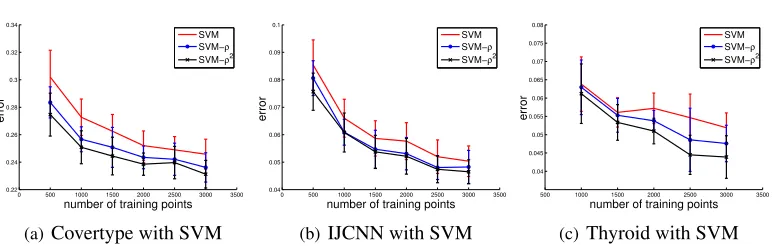
6.1 Feature Weighting for Support Vector Machines
Even though the intuition for our method has been developed for distance-based regressors and classifiers, we have found empirically that pre-processing features by multiplying them with their corresponding gradient weight also improves the performance of other popular classifiers, such as support vector machines (SVMs). This is demonstrated in Figure 8, which reports results on the same classification tasks as in Figure 5, but uses an SVM instead of ak-NN classifier. We have used a Gaussian kernel, and we have cross-validated its kernel bandwidthhseparately for the Euclidean and the learned metric space on half the training points. As before, h is found by a log search, followed by a linear search.
6.2 Relation to the Relief family of Heuristics
Early approaches for feature selection have exhaustively enumerated all possible subsets of features, or have employed heuristics to reduce the search space. In this section we relate our GW approach to the Relief approach, which from its introduction in Kira and Rendell (1992), has gained much popularity and evolved into a larger family of related heuristics (Kononenko, 1994; Robnik- ˇSikonja and Kononenko, 2003).
Covertype MAGIC Gamma Shuttle Page Blocks Gradient Weights 0.0113±0.0067 0.0050±0.0039 0.0006±0.0011 0.0007±0.0026 ReliefF 0.0229±0.0075 0.0147±0.0072 -0.0019±0.0024 -0.0019±0.0049
Table 3: Comparing the improvement in classification error over the k-NN baseline when using squared gradient weights or ReliefF shows that none of the two methods dominates the other one. Negative numbers indicate cases where ReliefF led to increased errors.
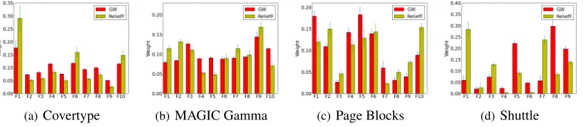
While Relief and our GW approach have similar practical benefits, GW is grounded in the the-oretical insights developed earlier in this work. Corollary 8 allows us to thethe-oretically understand the conditions under which GW improves regression rates in a minimax sense, opening up potential directions for further development of feature weighting methods. To the best of our knowledge, no such theoretical results are available for Relief although various works have provided theoretical interpretation (e.g. (Sun, 2007)) without actually analyzing the direct effect of Relief weights on regression or classification convergence rates. We will argue here that the theoretical intuition de-veloped in this work helps explain some of the success of Relief: the weights computed by Relief, similar to those of GW, are generally correlated with the coordinate-wise variation of the unknown regression functionf.
(a)Covertype (b)MAGIC Gamma (c) Page Blocks (d)Shuttle
Figure 9: Comparing GW feature weights (i.e.∇n,i) and those of ReliefF, averaged over 10 random
repeats of the experiment. There is a clear correlation in most cases but the right-most.
First, upon computing weights for several real-world data sets, we can observe empirically that the weights assigned by ReliefF (Kononenko, 1994) are often correlated with those computed by GW which are by design correlated with the coordinate-wise variation off (Figure 9).
Both methods, when used for feature-weighting, yield similar improvement in classification error rates, as shown in Table 3. For GW we use Wi = ∇2n,i, i.e. coordinates are weighted by ∇n,i; correspondingly, we pre-multiply features by their ReliefF weights as done in Wettschereck
et al. (1997). For a fair comparison, the numberkof neighbors used in ReliefF was found by cross-validation on the training data, just as in our method. None of the two methods dominates the other on all examples. However, unlike the weights found by ReliefF, gradient weights never led to an average increase in error.
![Figure 3: Typical gradient norms (estimates of ∥f′i∥1,µ , i ∈ [d]) for some real-world datasets.](https://thumb-us.123doks.com/thumbv2/123dok_us/9792437.1965002/7.612.109.502.89.205/figure-typical-gradient-norms-estimates-real-world-datasets.webp)