Regularized Policy Iteration
with Nonparametric Function Spaces
Amir-massoud Farahmand [email protected]
Mitsubishi Electric Research Laboratories (MERL) 201 Broadway, 8th Floor
Cambridge, MA 02139, USA
Mohammad Ghavamzadeh [email protected]
Adobe Research 321 Park Avenue
San Jose, CA 95110, USA
Csaba Szepesv´ari [email protected]
Department of Computing Science University of Alberta
Edmonton, AB, T6G 2E8, Canada
Shie Mannor [email protected]
Department of Electrical Engineering The Technion
Haifa 32000, Israel
Editor:Peter Auer
Abstract
We study two regularization-based approximate policy iteration algorithms, namely REG-LSPI and REG-BRM, to solve reinforcement learning and planning problems in discounted Markov Decision Processes with large state and finite action spaces. The core of these algorithms are the regularized extensions of the Least-Squares Temporal Difference (LSTD) learning and Bellman Residual Minimization (BRM), which are used in the algorithms’ policy evaluation steps. Regularization provides a convenient way to control the complexity of the function space to which the estimated value function belongs and as a result enables us to work with rich nonparametric function spaces. We derive efficient implementations of our methods when the function space is a reproducing kernel Hilbert space. We analyze the statistical properties of REG-LSPI and provide an upper bound on the policy evaluation error and the performance loss of the policy returned by this method. Our bound shows the dependence of the loss on the number of samples, the capacity of the function space, and some intrinsic properties of the underlying Markov Decision Process. The dependence of the policy evaluation bound on the number of samples is minimax optimal. This is the first work that provides such a strong guarantee for a nonparametric approximate policy iteration algorithm.1
Keywords: reinforcement learning, approximate policy iteration, regularization, non-parametric method, finite-sample analysis
1. Introduction
We study the approximate policy iteration (API) approach to find a close to optimal policy in a Markov Decision Process (MDP), either in a reinforcement learning (RL) or in a planning scenario. The basis of API, which is explained in Section3, is the policy iteration algorithm that iteratively evaluates a policy (i.e., finding the value function of the policy— the policy evaluation step) and then improves it (i.e., computing the greedy policy with respect to (w.r.t.) the recently obtained value function—the policy improvement step). When the state space is large (e.g., a subset of Rd or a finite state space that has too many states to be exactly represented), the policy evaluation step cannot be performed exactly, and as a result the use of function approximation is inevitable. The appropriate choice of the function approximation method, however, is far from trivial. The best choice is problem-dependent and it also depends on the number of samples in the input data.
In this paper we propose a nonparametric regularization-based approach to API. This approach provides a flexible and easy way to implement the policy evaluation step of API. The advantage of nonparametric methods over parametric methods is that they are flex-ible: Whereas a parametric model, which has a fixed and finite parameterization, limits the range of functions that can be represented, irrespective of the number of samples, the nonparametric models avoid such undue restrictions by increasing the power of the function approximation as necessary. Moreover, the regularization-based approach to nonparamet-rics is elegant and powerful: It has a simple algorithmic form and the estimator achieves minimax optimal rates in a number of scenarios. Further discussion of and specific re-sults about nonparametric methods, particularly in the supervised learning scenario, can be found in the books byGy¨orfi et al.(2002) andWasserman (2007).
The nonparametric approaches to solve RL/Planning problems have received some at-tention in the RL community. For instance,Petrik(2007);Mahadevan and Maggioni(2007); Parr et al. (2007); Mahadevan and Liu (2010); Geramifard et al. (2011); Farahmand and Precup(2012);B¨ohmer et al.(2013) andMilani Fard et al.(2013) suggest methods to gen-erate data-dependent basis functions, to be used in general linear models. Ormoneit and Sen (2002) use smoothing kernel-based estimate of the model and then use value iteration to find the value function. Barreto et al. (2011, 2012) benefit from “stochastic factoriza-tion trick” to provide computafactoriza-tionally efficient ways to scale up the approach of Ormoneit and Sen (2002). In the context of approximate value iteration,Ernst et al. (2005) consider growing ensembles of trees to approximate the value function. In addition, there have been some works where regularization methods have been applied to the RL/Planning prob-lems, e.g.,Engel et al.(2005);Jung and Polani(2006);Loth et al.(2007);Farahmand et al. (2009a,b);Taylor and Parr(2009);Kolter and Ng(2009);Johns et al.(2010);Ghavamzadeh et al.(2011);Farahmand(2011b);Avila Pires and Szepesv´´ ari(2012);Hoffman et al.(2012); Geist and Scherrer (2012). Nevertheless, most of these papers are algorithmic results and do not analyze the statistical properties of these methods (the exceptions are Farahmand et al. 2009a,b; Farahmand 2011b; Ghavamzadeh et al. 2011; Avila Pires and Szepesv´´ ari 2012). We compare these methods with ours in more detail in Sections 5.3.1and 6.
use greedy algorithms, such as Matching Pursuit (Mallat and Zhang,1993) and Orthogonal Matching Pursuit (Pati et al.,1993), to select features from a large set of features. Greedy algorithms have recently been developed for the value function estimation byJohns(2010); Painter-Wakefield and Parr(2012);Farahmand and Precup(2012);Geramifard et al.(2013). We do not discuss these methods any further.
1.1 Contributions
The algorithmic contribution of this work is to introduce two regularization-based nonpara-metric approximate policy iteration algorithms, namely Regularized Least-Squares Policy Improvement (REG-LSPI) and Regularized Bellman Residual Minimization (REG-BRM). These are flexible methods that, upon the proper selection of their parameters, are sample efficient. Each of REG-BRM and REG-LSPI is formulated as two coupled regularized op-timization problems (Section4). As we argue in Section4.1, having a regularized objective in both optimization problems is necessary for rich nonparametric function spaces. Despite the unusual coupled formulation of the underlying optimization problems, we prove that the solutions can be computed in a closed-form when the estimated action-value function belongs to the family of reproducing kernel Hilbert spaces (RKHS) (Section4.2).
The theoretical contribution of this work (Section 5) is to analyze the statistical prop-erties of REG-LSPI and to provide upper bounds on the policy evaluation error and the performance difference between the optimal policy and the policy returned by this method (Theorem 14). The result demonstrates the dependence of the bounds on the number of samples, the capacity of the function space to which the estimated action-value function belongs, and some intrinsic properties of the MDP. It turns out that the dependence of the policy evaluation error bound on the number of samples is minimax optimal. This pa-per, alongside its conference (Farahmand et al., 2009b) and the dissertation (Farahmand, 2011b) versions, is the first work that analyzes a nonparametric regularized API algorithm and provides such a strong guarantee for it.
2. Background and Notation
In the first part of this section, we provide a brief summary of some of the concepts and definitions from the theory of MDPs and RL (Section 2.1). For more information, the reader is referred to Bertsekas and Shreve (1978); Bertsekas and Tsitsiklis (1996); Sutton and Barto(1998);Szepesv´ari(2010). In addition to this background on MDPs, we introduce the notations we use to denote function spaces and their corresponding norms (Section2.2) as well as the considered learning problem (Section 2.3).
2.1 Markov Decision Processes
For a space Ω, with aσ-algebra σΩ, we define M(Ω) as the set of all probability measures overσΩ. We let B(Ω) denote the space of bounded measurable functions w.r.t. σΩ and we denote B(Ω, L) as the space of bounded measurable functions with bound 0< L <∞.
at (x, a) ∈ X × A gives a distribution over R× X, which we shall denote by P(·,·|x, a).
We denote the marginals of P by the overloaded symbol P : X × A → M(X) defined as
P(·|x, a) =Px,a(·) =
R
RP(dr,·|x, a) (transition probability kernel) andR:X × A → M(R)
defined as R(·|x, a) =R
XP(·, dy|x, a) (reward distribution).
An MDP together with an initial distributionP1of states encode the laws governing the temporal evolution of a discrete-time stochastic process controlled by an agent as follows: The controlled process starts at time t = 1 with random initial state X1 ∼ P1 (here and in what followsX∼Qdenotes that the random variableX is drawn from distributionQ). At stage t, actionAt∈ A is selected by the agent controlling the process. In response, the
pair (Rt, Xt+1) is drawn fromP(·,·|Xt, At), i.e., (Rt, Xt+1)∼P(·,·|Xt, At), where,Rtis the
reward that the agent receives at time t and Xt+1 is the state at time t+ 1. The process then repeats with the agent selecting actionAt+1, etc.
In general, the agent can use all past states, actions, and rewards in deciding about its current action. However, for our purposes it will suffice to consider action-selection procedures, or policies, that select an action deterministically and time-invariantly solely based on the current state:
Definition 2 (Deterministic Markov Stationary Policy) A measurable mapping π :
X → Ais called adeterministic Markov stationary policy, or justpolicyin short. Following a policy π in an MDP means that at each time step t it holds thatAt=π(Xt).
Policyπ induces the transition probability kernelsPπ :X × A → M(X × A) defined as follows: For a measurable subset C of X × A, let (Pπ)(C|x, a) ,R
P(dy|x, a)I{(y,π(y))∈C}.
The m-step transition probability kernels (Pπ)m :X × A → M(X × A) for m = 2,3,· · ·
are defined inductively by (Pπ)m(C|x, a),RXP(dy|x, a)(Pπ)m
−1(C|y, π(y)). Also given a probability transition kernel P :X × A → M(X × A), we define the right-linear operator
P·:B(X × A)→B(X × A) by (P Q)(x, a),R
X ×AP(dy, da
0|x, a)Q(y, a0). For a probability
measure ρ ∈ M(X × A) and a measurable subset C of X × A, we define the left-linear operators·P :M(X × A)→ M(X × A) by (ρP)(C) =R
ρ(dx, da)P(dy, da0|x, a)I{(y,a0)∈C}.
To study MDPs, two auxiliary functions are of central importance: the value and the
action-value functions of a policyπ.
Definition 3 (Value Functions) For a policy π, the value function Vπ and the action-value function Qπ are defined as follows: Let (Rt;t≥ 1) be the sequence of rewards when the Markov chain is started from a state X1 (or state-action (X1, A1) for the
action-value function) drawn from a positive probability distribution over X (or X × A) and
the agent follows policy π. Then, Vπ(x) , E h
P∞
t=1γt
−1R
t
X1 =x i
and Qπ(x, a) ,
E h
P∞
t=1γt−1Rt
X1 =x, A1 =a i
.
It is easy to see that for any policyπ, if the magnitude of the immediate expected reward
r(x, a) = Rr P(dr, dy|x, a) is uniformly bounded by Rmax, then the functionsVπ and Qπ
are bounded by Vmax=Qmax=Rmax/(1−γ), independent of the choice ofπ.
For a discounted MDP, we define theoptimal valueandoptimal action-valuefunctions by
state, i.e., ifVπ∗ =V∗. We say that a policyπ isgreedy w.r.t. an action-value functionQif
π(x) = argmaxa∈AQ(x, a) for allx ∈ X. We define function ˆπ(x;Q),argmaxa∈AQ(x, a)
(for all x ∈ X) that returns a greedy policy of an action-value function Q (If there exist multiple maximizers, a maximizer is chosen in an arbitrary deterministic manner). Greedy policies are important because a greedy policy w.r.t. the optimal action-value function Q∗
is an optimal policy. Hence, knowingQ∗is sufficient for behaving optimally (cf. Proposition 4.3 ofBertsekas and Shreve 1978).2
Definition 4 (Bellman Operators) For a policyπ, the Bellman operatorsTπ :B(X)→
B(X) (for value functions) and Tπ :B(X × A) → B(X × A) (for action-value functions) are defined as
(TπV)(x),r(x, π(x)) +γ
Z
X
V(y)P(dy|x, π(x)),
(TπQ)(x, a),r(x, a) +γ
Z
X
Q(y, π(y))P(dy|x, a).
To avoid unnecessary clutter, we use the same symbol to denote both operators. However, this should not introduce any ambiguity: Given some expression involving Tπ one can always determine which operatorTπ means by looking at the type of functionTπ is applied to. It is known that the fixed point of the Bellman operator is the (action-)value function of the policyπ, i.e.,TπQπ =Qπ and TπVπ =Vπ, see e.g., Proposition 4.2(b) ofBertsekas and Shreve (1978). We will also need to define the so-called Bellmanoptimalityoperators:
Definition 5 (Bellman Optimality Operators) The Bellman optimality operatorsT∗:
B(X) → B(X) (for value functions) and T∗ : B(X × A) → B(X × A) (for action-value functions) are defined as
(T∗V)(x),max
a
r(x, a) +γ
Z
X
V(y)P(dy|x, a)
,
(T∗Q)(x, a),r(x, a) +γ
Z
X
max
a0 Q(y, a
0)P(dy|x, a).
Again, we use the same symbol to denote both operators; the previous comment that no ambiguity should arise because of this still applies. The Bellman optimality operators enjoy a fixed-point property similar to that of the Bellman operators. In particular, T∗V∗ =V∗
and T∗Q∗ =Q∗, see e.g., Proposition 4.2(a) of Bertsekas and Shreve (1978). The Bellman optimality operator thus provides a vehicle to compute the optimal action-value function and therefore to compute an optimal policy.
2.2 Norms and Function Spaces
In what follows we use F :X →R to denote a subset of measurable functions. The exact specification of this set will be clear from the context. Further, we let F|A| :X × A →R|A|
to be a subset of vector-valued measurable functions with the identification of
F|A| =
(Q1, . . . , Q|A|) : Qi ∈ F, i= 1, . . . ,|A| .
We shall use kQkp,ν to denote the Lp(ν)-norm (1 ≤ p < ∞) of a measurable function
Q:X × A →R, i.e., kQkpp,ν ,R
X ×A|Q(x, a)|pdν(x, a).
Let z1:n denote the Z-valued sequence (z1, . . . , zn). ForDn=z1:n, define the empirical
norm of function f :Z →Ras
kfkpp,D
n =kfk
p p,z1:n ,
1
n
n
X
i=1
|f(zi)|p. (1)
When there is no chance of confusion about Dn, we may denote the empirical norm by kfkpp,n. Based on this definition, one may define kQkp,D
n with the choice of Z =X × A. Note that ifDn = (Zi)ni=1 is random with Zi ∼ν, the empirical norm is random too, and
for any fixed function f, we have E h
kfkp,D
n i
=kfkp,ν. When p = 2, we simply use k·kν
and k·kD
n.
2.3 Offline Learning Problem and Empirical Bellman Operators
We consider theoffline learning scenario when we are only given a batch of data3
Dn={(X1, A1, R1, X10), . . . ,(Xn, An, Rn, Xn0)}, (2)
with Xi ∼ νX, Ai ∼ πb(·|Xi), and (Ri, Xi0) ∼ P(·,·|Xi, Ai) for i = 1, . . . , n. Here νX ∈
M(X) is a fixed distribution over the states andπb is the data generating behavior policy,
which is a stochastic stationary Markov policy, i.e., given any state x ∈ X, it assigns a probability distribution over A. We shall also denote the common distribution underlying (Xi, Ai) byν ∈ M(X × A).
Samples Xi and Xi+1 may be sampled independently (we call this the “Planning
sce-nario”), or may be coupled through Xi0 = Xi+1 (“RL scenario”). In the latter case the data comes from a single trajectory. Under either of these scenarios, we say that the data
Dn meets the standard offline sampling assumption. We analyze the Planning scenario,
where the states are independent, but one may also analyze dependent processes by con-sidering mixing processes and using tools such as the independent blocks technique (Yu, 1994;Doukhan,1994), as has been done byAntos et al.(2008b);Farahmand and Szepesv´ari (2012).
The data set Dn allows us to define the so-called empirical Bellman operators, which can be thought of as empirical approximations to the true Bellman operators.
Definition 6 (Empirical Bellman Operators) Let Dn be a data set as above. Define the ordered multisetSn={(X1, A1), . . . ,(Xn, An)}. For a given fixed policyπ, the empirical Bellman operatorTˆπ :RSn →Rn is defined as
( ˆTπQ)(Xi, Ai),Ri+γQ(Xi0, π(Xi0)), 1≤i≤n .
Similarly, the empirical Bellman optimality operator Tˆ∗ :RSn →Rn is defined as
( ˆT∗Q)(Xi, Ai),Ri+γmax a0 Q(X
0
i, a0), 1≤i≤n .
In words, the empirical Bellman operators get an n-element list Sn and return an n
-dimensional real-valued vector of the single-sample estimate of the Bellman operators ap-plied to the action-value function Q at the selected points. It is easy to see that the empirical Bellman operators provide an unbiased estimate of the Bellman operators in the following sense: For any fixed bounded measurable deterministic function Q : X × A →
R, policy π and 1 ≤ i ≤ n, it holds that E h
ˆ
TπQ(Xi, Ai)|Xi, Ai
i
= TπQ(Xi, Ai) and
E h
ˆ
T∗Q(Xi, Ai)|Xi, Ai
i
=T∗Q(Xi, Ai).
3. Approximate Policy Iteration
The policy iteration algorithm computes a sequence of policies such that the new policy in the iteration is greedy w.r.t. the action-value function of the previous policy. This procedure requires one to compute the action-value function of the most recent policy (policy evaluation step) followed by the computation of the greedy policy (policy improvement step). In API, the exact, but infeasible, policy evaluation step is replaced by an approximate one. Thus, the skeleton of API methods is as follows: At thekthiteration and given a policyπk,
the API algorithm approximately evaluatesπk to find aQk. The action-value functionQk
is typically chosen to be such thatQk ≈TπkQk, i.e., it is an approximate fixed point ofTπk.
The API algorithm then calculates the greedy policy w.r.t. the most recent action-value function to obtain a new policyπk+1, i.e.,πk+1 = ˆπ(·;Qk). The API algorithm continues by
repeating this process again and generating a sequence of policies and their corresponding approximate action-value functions Q0 →π1 →Q1→π2→ · · ·.4
The success of an API algorithm hinges on the way the approximate policy evaluation step is implemented. Approximate policy evaluation is non-trivial for at least two reasons. First, policy evaluation is an inverse problem,5 so the underlying learning problem is unlike a standard supervised learning problem in which the data take the form of input-output pairs. The second problem is the off-policy sampling problem: The distribution of (Xi, Ai)
in the data samples (possibly generated by a behavior policy) is typically different from the distribution that would be induced if we followed the to-be-evaluated policy (i.e., target policy). This causes a problem since the methods must be able to handle this mismatch of
4. In an actual API implementation, one does not need to computeπk+1 for all states, which in fact is
infeasible for large state spaces. Instead, one usesQkto computeπk+1at some select states, as required
in the approximate policy evaluation step.
distributions.6 In the rest of this section, we review generic LSTD and BRM methods for approximate policy evaluation. We introduce our regularized version of LSTD and BRM in Section4.
3.1 Bellman Residual Minimization
The idea of BRM goes back at least to the work ofSchweitzer and Seidmann(1985). It was later used in the RL community byWilliams and Baird(1994) andBaird(1995). The basic idea of BRM comes from noticing that the action-value function is the unique fixed point of the Bellman operator: Qπ = TπQπ (or similarly Vπ = TπVπ for the value function). Whenever we replace Qπ by an action-value function Qdifferent from Qπ, the fixed-point equation would not hold anymore, and we have a non-zero residual functionQ−TπQ. This quantity is called the Bellman residual of Q. The same is true for the Bellman optimality operatorT∗.
The BRM algorithm minimizes the norm of the Bellman residual of Q, which is called the Bellman error. It can be shown that if kQ−T∗Qk is small, then the value function of the greedy policy w.r.t. Q, that is Vπˆ(·;Q), is also in some sense close to the optimal value functionV∗, see e.g.,Williams and Baird(1994);Munos(2003);Antos et al.(2008b); Farahmand et al.(2010), and Theorem 13 of this work. The BRM algorithm is defined as the procedure minimizing the following loss function:
LBRM(Q;π),kQ−TπQk2ν,
whereν is the distribution of state-actions in the input data. Using the empirical L2-norm defined in (1) with samples Dn defined in (2), and by replacing (TπQ)(Xt, At) with the
empirical Bellman operator (Definition 6), the empirical estimate of LBRM(Q;π) can be
written as
ˆ
LBRM(Q;π, n),
Q−
ˆ
TπQ
2
Dn = 1
n
n
X
t=1 h
Q(Xt, At)−
Rt+γQ Xt0, π(Xt0)
i2
. (3)
Nevertheless, it is well-known that ˆLBRM is not an unbiased estimate of LBRM when
the MDP is not deterministic (Lagoudakis and Parr,2003;Antos et al.,2008b). To address this issue,Antos et al. (2008b) propose the modified BRM loss that is a new empirical loss function with an extra de-biasing term. The idea of the modified BRM is to cancel the unwanted variance by introducing an auxiliary functionh and a new loss function
LBRM(Q, h;π) =LBRM(Q;π)− kh−TπQk2ν, (4)
and approximating the action-value function Qπ by solving
QBRM = argmin Q∈F|A|
sup
h∈F|A|
LBRM(Q, h;π), (5)
where the supremum comes from the negative sign of kh−TπQk2ν. They have shown that optimizing the new loss function still makes sense and the empirical version of this loss is unbiased.
The min-max optimization problem (5) is equivalent to the following coupled (nested) optimization problems:
h(·;Q) = argmin
h0∈F|A|
h0−TπQ 2
ν,
QBRM = argmin Q∈F|A|
h
kQ−TπQk2ν− kh(·;Q)−TπQk2νi. (6)
In practice, the norm k·kν is replaced by the empirical normk·kD
n andT
πQis replaced
by its sample-based approximation ˆTπQ, i.e.,
ˆ
hn(·;Q) = argmin h∈F|A|
h−
ˆ
TπQ
2
Dn
, (7)
ˆ
QBRM = argmin Q∈F|A|
h Q−
ˆ
TπQ
2
Dn
− ˆ
hn(·;Q)−TˆπQ
2
Dn i
. (8)
From now on, whenever we refer to the BRM algorithm, we are referring to this modified BRM.
3.2 Least-Squares Temporal Difference Learning
The Least-Squares Temporal Difference learning (LSTD) algorithm for policy evaluation was first proposed by Bradtke and Barto (1996), and later used in an API procedure by Lagoudakis and Parr(2003) and was called Least-Squares Policy Iteration (LSPI).
The original formulation of LSTD finds a solution to the fixed-point equation Q = ΠνTπQ, where Πν is the simplified notation for ν-weighted projection operator onto the
space of admissible functions F|A|, i.e., Πν , ΠF|A|
ν : B(X × A) → B(X × A) is defined by ΠF|A|
ν Q = argminh∈F|A|kh−Qk 2
ν for Q ∈ B(X × A). We, however, use a different
optimization-based formulation. The reason is that wheneverν is not the stationary distri-bution induced by π, the operator (ΠνTπ) does not necessarily have a fixed point, but the
optimization problem is always well-defined.
We define the LSTD solution as the minimizer of the L2-norm betweenQand ΠνTπQ:
LLST D(Q;π),kQ−ΠνTπQk2ν. (9)
The minimizer ofLLST D(Q;π) is well-defined, and wheneverνis the stationary distribution
ofπ (i.e., on-policy sampling), the solution to this optimization problem is the same as the solution to Q = ΠνTπQ. The LSTD solution can therefore be written as the solution to
the following set of coupled optimization problems:
h(·;Q) = argmin
h0∈F|A|
h0−TπQ 2
ν,
QLST D= argmin Q∈F|A|
Algorithm 1 Regularized Policy Iteration(K, ˆQ(−1),F|A|,J,{(λQ,n(k), λ(h,nk))}Kk=0−1) // K: Number of iterations
// ˆQ(−1): Initial action-value function // F|A|: The action-value function space
// J: The regularizer // {(λ(Q,nk), λ(h,nk))}K
k=0: The regularization coefficients for k= 0 to K−1 do
πk(·)←πˆ(·; ˆQ(k−1))
Generate training samplesDn(k)
ˆ
Q(k)← REG-LSTD/BRM(πk,D(nk);F|A|, J, λ(Q,nk), λ(h,nk))
end for
return Qˆ(K−1) and πK(·) = ˆπ(·; ˆQ(K−1))
where the first equation finds the projection ofTπQontoF|A|, and the second one minimizes
the distance of Q and the projection. The corresponding empirical version based on data set Dn is
ˆ
hn(·;Q) = argmin h∈F|A|
h−
ˆ
TπQ
2
Dn
, (11)
ˆ
QLST D= argmin Q∈F|A|
Q−
ˆ
hn(·;Q)
2
Dn
. (12)
For general spaces F|A|, these optimization problems can be difficult to solve, but when
F|A| is a linear subspace of B(X × A), the minimization problem becomes computationally feasible.
Comparison of BRM and LSTD is noteworthy. The population version of LSTD loss minimizes the distance betweenQand ΠνTπQ, which iskQ−ΠνTπQk2ν. Meanwhile, BRM
minimizes another distance function that is the distance between TπQ and ΠνTπQ
sub-tracted from the distance betweenQand TπQ, i.e.,kQ−TπQk2
ν− kˆhn(·;Q)−TπQk2ν. See
Figure 1a for a pictorial presentation of these distances. When F|A| is linear, because of
the Pythagorean theorem, the solution to the modified BRM (6) coincides with the LSTD solution (10) (Antos et al.,2008b).
4. Regularized Policy Iteration Algorithms
In this section we introduce two Regularized Policy Iteration algorithms, which are instances of the generic API algorithms. These algorithms are built on the regularized extensions of BRM (Section3.1) and LSTD (Section3.2) for the task of approximate policy evaluation.
The pseudo-code of the Regularized Policy Iteration algorithms is shown in Algorithm1. The algorithm receives K (the number of API iterations), an initial action-value function
ˆ
Minimized by original BRM
Minimized by LSTD
+ +
+ +
+ +
+ +
-
-
-
-
-
-
-
-(a)
Minimized by REG-BRM
Minimized by REG-LSTD + +
+ + + +
+ +
-
-
-
-
-
-
-
-(b)
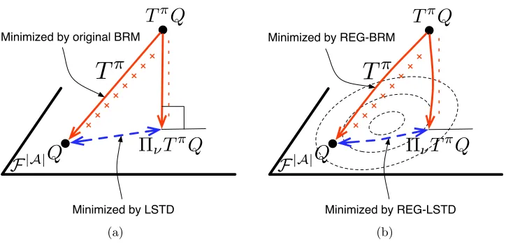
Figure 1: (a) This figure shows the loss functions minimized by the original BRM, the modified BRM, and the LSTD methods. The function spaceF|A| is represented by the plane. The Bellman operatorTπ maps an action-value function Q∈ F|A|
to a function TπQ. The function TπQ−ΠνTπQ is orthogonal to F|A|. The
original BRM loss function iskQ−TπQk2ν (solid line), the modified BRM loss is
kQ−TπQk2ν− kTπQ−ΠνTπQk2ν (the difference of two solid line segments; note
the + and−symbols), and the LSTD loss iskQ−ΠνTπQk2ν (dashed line). LSTD
and the modified BRM are equivalent for linear function spaces. (b) REG-LSTD and REG-BRM minimize regularized objective functions. Regularization makes the functionTπQ−ΠνTπQto be non-orthogonal to F|A|. The dashed ellipsoids
represent the level-sets defined by the regularization functionalJ.
πk ←πˆ(·; ˆQ(k−1) = argmaxa0∈AQˆ(k−1)(·, a0). For the first iteration (k= 0), one may ignore
this step and provide an initial policy π0 instead of ˆQ(−1). Afterwards, we have a data generating step: At each iteration k= 0, . . . , K−1, the agent follows the data generating policy πbk to obtain D
(k)
n = {(Xt(k), A
(k)
t , R
(k)
t , Xt0
(k)
)}1≤t≤n. For the kth iteration of the
algorithm, we use training samples Dn(k) to evaluate policyπk. In practice, one might want
to change πbk at each iteration in such a way that the agent ultimately achieves a better performance. The relation between the performance and the choice of data samples, however, is complicated. For simplicity of analysis, in the rest of this work we assume that a fixed behavior policy is used in all iterations, i.e., πbk =πb.
7 This leads toK independent data
setsDn(0), . . . ,D(K
−1)
n . From now on, to avoid clutter, we use symbolsDn, Xt, . . . instead of D(nk), Xt(k), . . . with the understanding that each Dn in various iterations is referring to an
independent set of data samples, which should be clear from the context.
The approximate policy evaluation step is performed by REG-LSTD/BRM, which will be discussed shortly. REG-LSTD/BRM receives policy πk, the training samples D
(k)
n , the
function space F|A|, the regularizer J, and the regularization coefficients (λ(k)
Q,n, λ
(k)
h,n), and
returns an estimate of the action-value function of policyπk. This procedure repeats for K
iterations.
REG-BRM approximately evaluates policy πk by solving the following coupled
opti-mization problems:
ˆ
hn(·;Q) = argmin h∈F|A|
h−
ˆ
TπkQ 2
Dn
+λ(h,nk)J2(h)
, (13)
ˆ
Q(k)= argmin
Q∈F|A|
Q−
ˆ
TπkQ 2
Dn
−
ˆ
hn(·;Q)−TˆπkQ
2
Dn
+λ(Q,nk)J2(Q)
, (14)
where J : F|A| →
R is the regularization functional (or simply regularizer or penalizer), and λ(h,nk), λ(Q,nk) >0 are regularization coefficients. The regularizer can be any pseudo-norm defined on F|A|; and Dn is defined as (2).8 The regularizer is often chosen such that
the functions that we believe are more “complex” have larger values of J. The notion of complexity, however, is subjective and depends on the choice of F|A| and J. Finally
note that we call J(Q) the smoothness of Q, even though it might not coincide with the conventional derivative-based notions of smoothness.
An example of the case thatJ has a derivative-based interpretation is when the function spaceF|A| is a Sobolev space and the regularizerJ is defined as its corresponding norm. In this case, we are penalizing the weak-derivatives of the estimate (Gy¨orfi et al.,2002;van de Geer, 2000). One can generalize the notion of smoothness beyond the usual derivative-based ones (cf. Chapter 1 of Triebel 2006) and define function spaces such as the family of Besov spaces (Devore, 1998). The RKHS norm for shift-invariant and radial kernels can also be interpreted as a penalizer of higher-frequency terms of the function (i.e., a low-pass filter Evgeniou et al. 1999), so they effectively encourage “smoother” functions. The choice of kernel determines the frequency response of the filter. One may also use other data-dependent regularizers such as manifold regularization (Belkin et al.,2006) and Sample-based Approximate Regularization (Bachman et al., 2014). As a final example, for the functions in the form ofQ(x, a) =P
i≥1φi(x, a)wi, if we choose a sparsity-inducing regularizer such asJ(Q),P
i≥1|wi|as the measure of smoothness, then a function that has
a sparse representation in the dictionary{φi}i≥1 is, by definition, a smooth function—even though there is not necessarily any connection to the derivative-based smoothness.
REG-LSTD approximately evaluates the policy πk by solving the following coupled
optimization problems:
ˆ
hn(·;Q) = argmin h∈F|A|
h−
ˆ
TπkQ 2
Dn
+λ(h,nk)J2(h)
, (15)
ˆ
Q(k)= argmin
Q∈F|A|
Q−
ˆ
hn(·;Q)
2
Dn
+λ(Q,nk)J2(Q)
. (16)
Note that the difference between (7)-(8) ((11)-(12)) and (13)-(14) ((15)-(16)) is the addition of the regularizersJ2(h) andJ2(Q).
Unlike the non-regularized case described in Section 3, the solutions of REG-BRM and REG-LSTD are not the same. As a result of the regularized projection, (13) and
(15), the function ˆhn(·;Q)−TˆπkQ is not orthogonal to the function space F|A|—even if F|A| is a linear space. Therefore, the Pythagorean theorem is not applicable anymore:
kQ−ˆhn(·;Q)k26=kQ−TˆπkQk2− kˆhn(·;Q)−TˆπkQk2 (See Figure1b).
One may ask why we have regularization terms in both optimization problems, as op-posed to only in the projection term (15) (similar to the Lasso-TD algorithm Kolter and Ng 2009; Ghavamzadeh et al. 2011) or only in (16) (similar to Geist and Scherrer 2012;
´
Avila Pires and Szepesv´ari 2012). We discuss this question in Section4.1. Briefly speaking, for large function spaces such as the Sobolev spaces or the RKHS with universal kernels, if we remove the regularization term in (15), the coupled optimization problems reduces to (unmodified) BRM, which is biased as discussed earlier; whereas if the regularization term in (16) is removed, the solution can be arbitrary bad due to overfitting.
Finally note that the choice of the function space F|A|, the regularizer J, and the regularization coefficients λ(Q,nk) and λ(h,nk) all affect the sample efficiency of the algorithms. If one knew J(Qπ), the regularization coefficients could be chosen optimally. Nonetheless, the value of J(Qπ) is often not known, so one has to use a model selection procedure to set the best function space and the regularization coefficients. The situation is similar to the problem of model selection in supervised learning (though the solutions are different). After developing some tools necessary for discussing this issue in Section5, we return to the problem of choosing the regularization coefficients after Theorem11as well as in Section6.
Remark 7 To the best of our knowledge, Antos et al. (2008b) were the first who explicitly considered LSTD as the optimizer of the loss function (9). Their discussion was mainly to prove the equivalence of modified BRM (5) and LSTD whenF|A| is a linear function space. In their work, the loss function is not used to derive any new algorithm. Farahmand et al.
(2009b) used this loss function to develop the regularized variant of LSTD (15)-(16). This loss function was later called mean-square projected Bellman error by Sutton et al.(2009), and was used to derive the GTD2 and TDC algorithms.
4.1 Why Two Regularizers?
We discuss why using regularizers in both optimization problems (15) and (16) of REG-LSTD is necessary for large function spaces such as the Sobolev spaces and the RKHS with universal kernels. Here we show that for large function spaces, depending on which regularization term we remove, either the coupled optimization problems reduces to the regularized variant of the unmodified BRM, which has a bias, or the solution can be arbitrary bad.
Let us focus on REG-LSTD for a given policy π. Assume that the function space
Case 1. In this case, we only regularize the empirical error kQ−ˆhn(·;Q)k2Dn, but we do not regularize the projection, i.e.,
ˆ
hn(·;Q) = argmin h∈F|A|
h−
ˆ
TπQ
2 Dn , ˆ
Q= argmin
Q∈F|A|
Q−
ˆ
hn(·;Q)
2
Dn
+λQ,nJ2(Q)
. (17)
When the function space F|A| is rich enough, there exists a function ˆh
n ∈ F|A| that fits
perfectly well to its target values at data points {(Xi, Ai)}ni=1, that is, ˆhn((Xi, Ai);Q) =
( ˆTπQ)(Xi, Ai) fori= 1, . . . , n.9 Such a function is indeed the minimizer of the loss kQ−
ˆ
hn(·;Q)k2Dn. The second optimization problem (17) becomes
ˆ
Q= argmin
Q∈F|A|
Q−Tˆ
πQ 2
Dn
+λQ,nJ2(Q)
.
This is the regularized version of the original (i.e., unmodified) formulation of the BRM algorithm. As discussed in Section 3.1, the unmodified BRM algorithm is biased when the MDP is not deterministic. Adding a regularizer does not solve the biasedness problem of the unmodified BRM loss. So without regularizing the first optimization problem, the function ˆ
hn overfits to the noise and as a result the whole algorithm becomes incorrect.
Case 2. In this case, we only regularize the empirical projection kh−TˆπQk2
Dn, but we do not regularize kQ−ˆhn(·;Q)k2Dn, i.e.,
ˆ
hn(·;Q) = argmin h∈F|A|
h−
ˆ
TπQ
2
Dn
+λh,nJ2(h)
,
ˆ
Q= argmin
Q∈F|A|
Q−
ˆ
hn(·;Q)
2 Dn . (18)
For a fixed Q, the first optimization problem is the standard regularized regression es-timator with the regression functionE
h
( ˆTπQ)(X, A)|X=x, A=a
i
= (TπQ)(x, a).
There-fore, if the function space F|A| is rich enough and we set the regularization coefficientλh,n
properly,kh−TπQkν andkh−TπQkDn go to zero as the sample size grows (the rate of con-vergence depends on the complexity of the target function; cf. Lemma15and Theorem16). So we can expect ˆhn(·;Q) to get closer toTπQas the sample size grows.
For simplicity of discussion, suppose that we are in the ideal situation where for any Q, we have ˆhn((x, a);Q) = (TπQ)(x, a) for all (x, a) ∈ {(Xi, Ai)}ni=1∪ {(Xi0, π(Xi0))}ni=1, that 9. To be more precise: First, for an ε > 0, we construct a continuous function ¯hε(z) =
P
Zi∈{(Xi,Ai)}ni=1max
n
1−kz−Zik
ε ,0
o
( ˆTπQ)(Zi).We then use the denseness of the function spaceF|A|
in the supremum norm to argue that there existshε∈ F|A|
such thathε−¯hε
∞ is arbitrarily close to
zero. So whenε→0, the value of functionhεis arbitrarily close toTπQat data points. We then choose ˆ
is, we precisely knowTπQat all data points.10 Substituting this ˆhn((x, a);Q) in the second
optimization problem (17), we get that we are solving the following optimization problem:
ˆ
Q= argmin
Q∈F|A|
kQ−TπQk2D
n. (19)
This is the Bellman error minimization problem. We do not have the biasedness problem here as we have TπQ instead of ˆTπQ in the loss. Nonetheless, we face another problem:
Minimizing this empirical risk minimization without controlling the complexity of the func-tion space might lead to an overfitted solufunc-tion, very similar to the same phenomenon in supervised learning.
To see it more precisely, we first construct a continuous function
¯
Qε(z) =
X
Zi∈{(Xi,Ai)}ni=1∪{(Xi0,π(Xi0))}ni=1
max
1−kz−Zik
ε ,0
Qπ(Zi),
which for small enough ε > 0 has the property that Q¯ε−TπQ¯ε 2
Dn is zero, i.e., it is a minimizer of the empirical loss. Due to the denseness of F|A|, we can find a Qε ∈ F|A|
that is arbitrarily close to the continuous function ¯Qε. Therefore, for small enough ε, the
functionQε is a minimizer of (19), i.e., the value ofkQε−TπQεk2Dn is zero. But Qε is not a good approximation of Qπ because Qε consists of spikes in the ε-neighbourhood of data
points and zero elsewhere. In other words, Qε does not generalize well beyond the data
points when εis chosen to be small.
Of course the solution is to control the complexity of F|A| so that spiky functions such as Qε are not selected as the solution of the optimization problem. When we regularize
both optimization problems, as we do in this work, none of these problems happen. This argument applies to rich function spaces that can approximate any reasonably complex functions (e.g., continuous functions) arbitrarily well. If the function space F|A|
is much more limited, for example if it is a parametric function space, we may not need to regularize both optimization problems. An example of such an approach for parametric spaces has been analyzed byAvila Pires and Szepesv´´ ari(2012).
4.2 Closed-Form Solutions
In this section we provide a closed-form solution for (13)-(14) and (15)-(16) for two cases: 1) WhenF|A|is a finite dimensional linear space andJ2(·) is defined as the weighted squared sum of parameters describing the function (a setup similar to the ridge regressionHoerl and Kennard 1970) and 2)F|A| is an RKHS and J(·) is the corresponding inner-product norm, i.e., J2(·) = k·k2H. Here we use a generic π and Dn instead of πk and Dn(k) at the kth
iteration.
10. This is an ideal situation because 1)kh−TˆπQkν is equal to zero only asymptotically and not in finite samples regime, and 2) even ifkh−Tˆπ
4.2.1 A Parametric Formulation for REG-BRM and REG-LSTD
In this section we consider the case whenh andQ are both given as linear combinations of some basis functions:
h(·) =φ(·)>u, Q(·) =φ(·)>w, (20)
where u,w ∈ Rp are parameter vectors and φ(·) ∈
Rp is a vector of p linearly indepen-dent basis functions defined over the space of state-action pairs.11 These basis functions might be predefined (e.g., Fourier (Konidaris et al.,2011) or wavelets) or constructed data-dependently by one of already mentioned feature generation methods. We further assume that the regularization terms take the form
J2(h) =u>Ψu, J2(Q) =w>Ψw.
for some user-defined choice of positive definite matrix Ψ∈Rp×p. A simple and common
choice would be Ψ=I. Define Φ,Φ0 ∈Rn×p and r∈Rn as follows: Φ=φ(Z1), . . . ,φ(Zn)
>
,Φ0=φ(Z10), . . . ,φ(Zn0)
>
,r=R1, . . . , Rn
>
, (21)
withZi = (Xi, Ai) and Zi0 = (Xi0, π(Xi0)).
The solution to REG-BRM is given by the following proposition.
Proposition 8 (Closed-form solution for REG-BRM) Under the setting of this sec-tion, the approximate action-value function returned by REG-BRM is Qˆ(·) = φ(·)>w∗, where
w∗=hB>B−γ2C>C+nλQ,nΨ
i−1
B>+γC>(ΦA−I)r,
with A= Φ>Φ+nλh,nΨ
−1
Φ>, B=Φ−γΦ0, C = (ΦA−I)Φ0.
Proof Using (20) and (21), we can rewrite (13)-(14) as u∗(w) = argmin
u∈Rp
1
n
Φu−(r+γΦ0w)>
Φu−(r+γΦ0w)
+λh,nu>Ψu
, (22)
w∗ = argmin
w∈Rp
1
n
Φw−(r+γΦ0w)>
Φw−(r+γΦ0w)
− (23)
1
n
Φu∗(w)−(r+γΦ0w)>Φu∗(w)−(r+γΦ0w)+λQ,nw>Ψw
.
Taking the derivative of (22) w.r.t. u and equating it to zero, we obtain u∗ as a function of w:
u∗(w) =Φ>Φ+nλh,nΨ
−1
Φ>(r+γΦ0w) =A(r+γΦ0w). (24) Plugu∗(w) from (24) into (23), take the derivative w.r.t. wand equate it to zero to obtain the parameter vector w∗ as announced above.
The solution returned by REG-LSTD is given in the following proposition.
Proposition 9 (Closed-form solution for REG-LSTD) Under the setting of this sec-tion, the approximate action-value function returned by REG-LSTD is Qˆ(·) = φ(·)>w∗, where
w∗ =hE>E+nλQ,nΨ
i−1
E>Ar,
with A= Φ>Φ+nλh,nΨ
−1
Φ> and E = (Φ−γAΦ0).
Proof Using (20) and (21), we can rewrite (15)-(16) as
u∗(w) = argmin
u∈Rp
1
n
Φu−(r+γΦ0w)>Φu−(r+γΦ0w)+λh,nu>Ψu
, (25)
w∗ = argmin
w∈Rp
n
Φw−Φu∗(w)>
Φw−Φu∗(w)
+λQ,nw>Ψw
o
. (26)
Similar to the parametric REG-BRM, we solve (25) and obtainu∗(w) which is the same as (24). If we plug this u∗(w) into (26), take derivate w.r.t. w, and find the minimizer, the parameter vectorw∗ will be as announced.
4.2.2 RKHS Formulation for REG-BRM and REG-LSTD
The class of reproducing kernel Hilbert spaces provides a flexible and powerful family of function spaces to choose F|A| from. An RKHS H : X × A →
R is defined by a positive definite kernelk: (X ×A)×(X ×A)→R. With such a choice, we can use the corresponding squared RKHS normk·k2Has the regularizerJ2(·). REG-BRM with an RKHS function space
F|A| =H would be
ˆ
hn(·;Q) = argmin h∈F|A|[=H]
h−
ˆ
TπQ
2
Dn
+λh,nkhk2H
, (27)
ˆ
Q= argmin
Q∈F|A|[=H]
Q−
ˆ
TπQ
2 Dn − ˆ
hn(·;Q)−TˆπQ
2
Dn
+λQ,nkQk2H
, (28)
and the coupled optimization problems for REG-LSTD are
ˆ
hn(·;Q) = argmin h∈F|A|[=H]
h−
ˆ
TπQ
2
Dn
+λh,nkhk2H
, (29)
ˆ
Q= argmin
Q∈F|A|[=H]
Q−ˆhn(·;Q) 2
Dn
+λQ,nkQk2H
. (30)
We can solve these coupled optimization problems by the application of the generalized representer theorem for RKHS (Sch¨olkopf et al.,2001). The result, which is stated in the next theorem, shows that the infinite dimensional optimization problem defined onF|A| =H
boils down to a finite dimensional problem with the dimension twice the number of data points.
˜
α∈R2n. The same holds for the solution to (29)-(30). Further, the coefficient vectors can be obtained in the following form:
REG-BRM: α˜BRM= (CKQ+nλQ,nI)−1(D>+γC>2B>B)r,
REG-LSTD: α˜LSTD= (F>F KQ+nλQ,nI)−1F>Er,
where r = (R1, . . . , Rn)> and the matrices KQ,B,C,C2,D,E,F are defined as follows: Kh ∈Rn×n is defined as [Kh]ij =k(Zi, Zj), 1 ≤i, j ≤n, and KQ∈R2n×2n is defined as [KQ]ij = k( ˜Zi,Z˜j), 1 ≤i, j ≤ 2n. Let C1 = In×n 0n×n
and C2 = 0n×n In×n
. Denote D = C1 −γC2, E = Kh(Kh+nλh,nI)−1, F = C1 −γEC2, B = Kh(Kh+
nλh,nI)−1−I, and C =D>D−γ2(BC2)>(BC2). Proof See Appendix A.
5. Theoretical Analysis
In this section, we analyze the statistical properties of REG-LSPI and provide a finite-sample upper bound on the performance losskQ∗−QπKk
1,ρ. Here,πK is the policy greedy
w.r.t. ˆQ(K−1) and ρ is the performance evaluation measure. The distributionρ is chosen by the user and is often different from the sampling distributionν.
Our study has two main parts. First, we analyze the policy evaluation error of REG-LSTD in Section5.1. We suppose that given any policyπ, we obtain ˆQby solving (15)-(16) with πk in these equations being replaced by π. Theorem 11 provides an upper bound
on the Bellman error kQˆ −TπQˆkν. We discuss the optimality of this upper bound for
policy evaluation for some general classes of function spaces. We show that the result is not only optimal in its convergence rate, but also in its dependence on J(Qπ). After that in Section5.2, we show how the Bellman errors of the policy evaluation procedure propagate through the API procedure (Theorem13). The main result of this paper, which is an upper bound on the performance loss kQ∗−QπKk
1,ρ, is stated as Theorem 14 in Section 5.3,
followed by its discussion. We compare this work’s statistical guarantee with some other papers’ in Section5.3.1.
To analyze the statistical performance of the REG-LSPI procedure, we make the follow-ing assumptions. We discuss their implications and the possible relaxations after statfollow-ing each of them.
Assumption A1 (MDP Regularity) The set of states X is a compact subset of Rd. The random immediate rewards Rt ∼ R(·|Xt, At) (t = 1,2, . . .) as well as the expected
immediate rewards r(x, a) are uniformly bounded by Rmax, i.e., |Rt| ≤Rmax (t= 1,2, . . .) and krk∞≤Rmax.
metrizable topological space. Nevertheless, we do not investigate such generalizations here. The boundedness of the rewards is a reasonable assumption that can be replaced by a more relaxed condition such as its sub-Gaussianity (Vershynin, 2012;van de Geer, 2000). This relaxation, however, increases the technicality of the proofs without adding much to the intuition. We remark on the compactness assumption after stating Assumption A4.
Assumption A2 (Sampling) At iteration k of REG-LSPI (for k = 0, . . . , K −1), n
fresh independent and identically distributed (i.i.d.) samples are drawn from distribution
ν ∈ M(X × A), i.e., Dn(k) =
n
Zt(k), Rt(k), Xt0(k)on
t=1 with Z (k)
t = (X
(k)
t , A
(k)
t )
i.i.d.
∼ ν and
Xt0(k)∼P(·|Xt(k), A(tk)).
The i.i.d. requirement of Assumption A2is primarily used to simplify the proofs. With much extra effort, these results can be extended to the case when the data samples belong to a single trajectory generated by a fixed policy. In the single trajectory scenario, samples are not independent anymore, but under certain conditions on the Markov process, the process (Xt, At) gradually “forgets” its past. One way to quantify this forgetting is through
mixing processes. For these processes, tools such as the independent blockstechnique (Yu, 1994; Doukhan, 1994) or information theoretical inequalities (Samson, 2000) can be used to carry on the analysis—as have been done by Antos et al. (2008b) in the API context, byFarahmand and Szepesv´ari (2012) for analyzing the regularized regression problem, and by Farahmand and Szepesv´ari(2011) in the context of model selection for RL problems.
It is worthwhile to emphasize that we do not require that the distributionνto be known. The sampling distribution is also generally different from the distribution induced by the target policy πk. For example, it might be generated by drawing state samples from a
givenνX and choosing actions according to a behavior policyπb, which is different from the
policy being evaluated. So we are in the off-policy sampling setting. Moreover, changing
ν at each iteration based on the previous iterations is a possibility with potential practical benefits, which has theoretical justifications in the context of imitation learning (Ross et al., 2011). For simplicity of the analysis, however, we assume that ν is fixed in all iterations. Finally, we note that the proofs work fine if we reuse the same data sets in all iterations. We comment on it later after the proof of Theorem11 in AppendixB.
Assumption A3 (Regularizer) Define two regularization functionalsJ :B(X)→Rand
J :B(X × A) →Rthat are pseudo-norms on F and F|A|, respectively.12 For allQ∈ F|A|
and a∈ A, we haveJ(Q(·, a))≤J(Q).
The regularizer J(Q) measures the complexity of an action-value function Q. The functions that are more complex have larger values ofJ(Q). We also need to define a related regularizer for value functions Q(·, a) (a∈ A). The latter regularizer is not explicitly used in the algorithm, and is only used in the analysis. This assumption imposes some mild restrictions on these regularization functionals. The condition that the regularizers be pseudo-norms is satisfied by many commonly-used regularizers such as the Sobolev norms,
the RKHS norms, and the l2-regularizer defined in Section 4.2.1 with a positive semi-definite choice of matrix Ψ. Moreover, the condition J(Q(·, a)) ≤ J(Q) essentially states that the complexity of Q should upper bound the complexity of Q(·, a) for all a ∈ A. If the regularizer J : B(X × A) → R is derived from a regularizer J0 :B(X) → R through
J(Q) = k(J0(Q(·, a))a∈Akp for some p ∈ [1,∞], then J will satisfy the second part of the
assumption. From a computational perspective, a natural choice for RKHS is to choose
p= 2 and to defineJ2(Q) =P
a∈AkQ(·, a)k
2
H forHbeing the RKHS defined onX.
Assumption A4 (Capacity of Function Space) ForR >0, let FR={f ∈ F :J(f)≤
R}. There exist constantsC > 0 and 0< α < 1 such that for any u, R >0 the following metric entropy condition is satisfied:
logN∞(u,FR)≤C
R u
2α
.
This assumption characterizes the capacity of the ball with radius R in F. The value of
α is an essential quantity in our upper bounds. The metric entropy is precisely defined in Appendix G, but roughly speaking it is the logarithm of the minimum number of balls with radius u that are required to completely cover a ball with radius R in F. This is a measure of complexity of a function space as it is more difficult to estimate a function when the metric entropy grows fast when u decreases. As a simple example, when the function space is finite, we effectively need to have good estimate of |F | functions in order not to choose the wrong one. In this case, N∞(u,FR) can be replaced by |F |, so α = 0
and C = log|F |. When the state space X is finite and all functions are bounded by
Qmax, we have logN∞(u,FR)≤logN∞(u,F) =|X |log(2Qumax). This shows that the metric
entropy for problems with finite state spaces grows much slower than what we consider here. Assumption A4 is suitable for large function spaces and is indeed satisfied for the Sobolev spaces and various RKHS. Refer to van de Geer(2000); Zhou (2002,2003); Steinwart and Christmann(2008) for many examples.
An alternative assumption would be to have a similar metric entropy for the balls in
F|A| (instead of F). This would slightly change a few steps of the proofs, but leave the
results essentially the same. Moreover, it makes the requirement thatJ(Q(·, a))≤J(Q) in AssumptionA3 unnecessary. Nevertheless, as results on the capacity ofF is more common in the statistical learning theory literature, we stick to the combination of Assumptions A3 and A4.
The metric entropy here is defined w.r.t. the supremum norm. All proofs, except that of Lemma 23, only require the same bound to hold when the supremum norm is replaced by the more relaxed empiricalL2-norm, i.e., those results require that there exist constants
C > 0 and 0 < α < 1 such that for any u, R > 0 and all x1, . . . , xn ∈ X, we have
logN2(u,FR, x1:n) ≤ C Ru
2α
. Of course, the metric entropy w.r.t. the supremum norm implies the one with the empirical norm. It is an interesting question to relax the supremum norm assumption in Lemma 23.
So we could remove the compactness requirement from Assumption A1 and implicitly let Assumption A4 satisfy it, but we preferred to be explicit about it at the cost of a bit of redundancy in our set of assumptions.
Assumption A5 (Function Space Boundedness) The subsetF|A| ⊂B(X × A;Qmax) is a separable and complete Carath´eodory set with Rmax≤Qmax<∞.
Assumption A5 requires all the functions in F|A| to be bounded so that the solutions of optimization problems (15)-(16) stay bounded. If they are not, they should be truncated, and thus, the truncation argument should be used in the analysis, see e.g., the proof of Theorem 21.1 of Gy¨orfi et al.(2002). The truncation argument does not change the final result, but complicates the proof at several places, so we stick to the above assumption to avoid unnecessary clutter. Moreover, in order to avoid the measurability issues resulting from taking supremum over an uncountable function spaceF|A|, we require the space to be a separable and complete Carath´eodory set (cf. Section 7.3 of Steinwart and Christmann 2008).
Assumption A6 (Function Approximation Property) The action-value function of any policyπ belongs to F|A|, i.e.,Qπ ∈ F|A|.
This “no function approximation error” assumption is standard in analyzing regularization-based nonparametric methods. This assumption is realistic and is satisfied for rich function spaces such as RKHS defined by universal kernels, e.g., Gaussian or exponential kernels (Section 4.6 of Steinwart and Christmann 2008). On the other hand, if the space is not large enough, we might have function approximation error. The behavior of the function approximation error for certain classes of “small” RKHS has been discussed bySmale and Zhou (2003); Steinwart and Christmann (2008). We stick to this assumption to simplify many key steps in the proofs.
Assumption A7 (Expansion of Smoothness) For all Q∈ F|A|, there exist constants 0≤LR, LP <∞, depending only on the MDP andF|A|, such that for policy π,
J(TπQ)≤LR+γLPJ(Q).
We require that the complexity ofTπQto be comparable to the complexity ofQ itself. In other words, we require that ifQis smooth according to the regularizerJof a function space
F|A|, it stays smooth after the application of the Bellman operator. We believe that this is
a reasonable assumption for many classes of MDPs with “sufficient” stochasticity and when
F|A| is rich enough. The intuition is that if the Bellman operator has a “smoothing” effect, the norm ofTπQdoes not blow up and the function can still be represented well withinF|A|.
Proposition 25 in Appendix F presents the conditions that for the so-called convolutional
5.1 Policy Evaluation Error
In this section, we focus on thekth iteration of REG-LSPI. To simplify the notation, we use
Dn={(Zt, Rt, Xt0)}nt=1 to refer toD (k)
n . The policy πk depends on data used in the earlier
iterations, but since we use independent set of samples D(nk) for the kth iteration andπk is
independent ofD(nk), we can safely ignore the randomness ofπkby working on the probability
space obtained by conditioning on Dn(0), . . . ,D(nk−1), i.e., the probability space used in the
kth iteration is (Ω, σΩ,Pk) with Pk =P n
· D
(0)
n , . . . ,D(k
−1)
n
o
. In order to avoid clutter, we do not use the conditional probability symbol. In the rest of this section, π refers to a
σ(D(0)n , . . . ,D(k
−1)
n )-measurable policy and is independent of Dn; ˆQ and ˆhn(Q) = ˆhn(·;Q)
refer to the solution to (15)-(16) whenπ,λh,n, and λQ,n replace πk,λ(h,nk), and λ(Q,nk) in that
set of equations, respectively.
The following theorem is the main result of this section and provides an upper bound on the statistical behavior of the policy evaluation procedure REG-LSTD.
Theorem 11 (Policy Evaluation) For any fixed policy π, let Qˆ be the solution to the optimization problem (15)-(16) with the choice of
λh,n=λQ,n =
1
n J2(Qπ)
1+1α
.
If Assumptions A1–A7 hold, there exists c(δ) >0 such that for any n∈ N and 0< δ <1, we have
ˆ
Q−TπQˆ
2
ν
≤c(δ)n−1+1α,
with probability at least 1−δ. Here c(δ) is equal to
c(δ) =c1 1 + (γLP)2
J1+2αα(Qπ) ln(1/δ) +c2 L
2α
1+α
R +
L2R
[J(Qπ)]1+2α !
,
for some constants c1, c2 >0.
Theorem 11, which is proven in Appendix B, indicates how the number of samples and the difficulty of the problem as characterized by J(Qπ), LP, and LR influence the policy
evaluation error.13
This upper bound provides some insights about the behavior of the REG-LSTD al-gorithm. To begin with, it shows that under the specified conditions, REG-LSTD is a consistent algorithm: As the number of samples increases, the Bellman error decreases and asymptotically converges to zero. This is due to the use of a nonparametric function space and the proper control of its complexity through regularization. A parametric function space, e.g., a linear function approximator with a fixed number of features, does not gen-erally have a similar guarantee unless the value function happens to belong to the span of the features. Achieving consistency for parametric function spaces requires careful choice
of features, and might be difficult. On the other hand, a rich enough nonparametric func-tion space, for example one defined by a universal kernel (cf. Assumpfunc-tionA6), ensures the consistency of the policy evaluation algorithm.
This theorem, however, is much more powerful than a consistency result as it provides a finite-sample upper bound guarantee for the error, too. If the parameters of the REG-LSTD algorithm are selected properly, one may achieve the sample complexity upper bound ofO(n−1/(1+α)). For the case of the Sobolev spaceWk(X) withX being an open Euclidean ball in Rd and k > d/2, one may choose α = d/2k to obtain the error upper bound of
O(n−d/(2k+d)).14
To study the upper bound a bit closer, let us focus on the special case ofγ = 0. For this choice of the discount factor,TπQis equal torπ and ( ˆTπQ)(Xi, Ai) is equal toRi. One can
see that the policy evaluation problem becomes a regression problem with the regression function rπ. The guarantee of this theorem would be then on kQˆ−TπQˆk2
ν =kQˆ−rπk2ν,
which is the usual squared error in the regression literature. Hence we reduced a regression problem to a policy evaluation problem. Because of this reduction, any lower bound on the regression would also be a lower bound on the policy evaluation problem.
It is well-known that the convergence rate ofn−d/(2k+d)is asymptotically minimax opti-mal for the regression estimation for target functions belonging to the Sobolev spaceWk(X) as well as some other smoothness classes with the k order of smoothness, cf. e.g., Nuss-baum(1999) for the results for the Sobolev spaces,Stone(1982) for a closely related H¨older space Cp,α, which with the choice ofk =p+α (k∈N and 0< α ≤1) has the same rate, andTsybakov(2009) for several results on minimax optimality of nonparametric estimators. More generally, the rate ofO(n−1/(1+α) is optimal too: For a regression function belonging to a function space F with a packing entropy in the same form as in the upper bound of Assumption A4, the rate Ω(n−1/(1+α)) is its minimax lower bound (Yang and Barron, 1999), making the upper bound optimal. Comparing these lower bounds with the upper boundO(n−1/(1+α)) (orO(n−d/(2k+d)) for the Sobolev space) of this theorem indicates that REG-LSTD algorithm has the optimal error rate as a function of the number of samplesn, which is a remarkable result.
Furthermore, to understand the fine behavior of the upper bound, beyond the depen-dence of the rate onn and α, we focus on the multiplicative term c(δ). Again we consider the special case of regression estimation as it is the only case we have some known lower bounds. With the choice of γ = 0, we have Qπ =rπ, so J(Qπ) = J(rπ). Moreover, since
TπQ = rπ + 0PπQ = rπ, we can choose L
R = J(rπ) in Assumption A7. As a result
c(δ) = c1 J
2α
1+α(rπ) ln(1/δ) for a constant c1 > 0. We are interested in studying the de-pendence of the upper bound on J(rπ). We study its behavior when the function space is the Sobolev spaceWk([0,1]) andJ(·) is the corresponding Sobolev space norm. We choose
α = 1/2k to get J2k2+1(rπ) dependence of c(δ). On the other hand, for the regression
es-timation problem within the subset F1|A|=Q(·, a)∈Wk([0,1]) : J(Q)≤J(rπ),∀a∈ A of this Sobolev space, the fine behavior of the asymptotic minimax rate is determined by
the so-called Pinsker constant, whose dependence on J is in fact J2k2+1(rπ), cf. e.g.,
Nuss-baum (1999,1985); Golubev and Nussbaum (1990), or Section 3.1 of Tsybakov (2009).15 Therefore, not only the exponent of the rate is optimal for this function space, but also its multiplicative dependence on the smoothness J(rπ) is optimal.
For function spaces other than this choice of Sobolev space (i.e., the general case ofα), we are not aware of any refined lower bound that indicates the optimality ofJ1+2αα(rπ). We note that some available upper bounds for regression with comparable assumptions on the metric entropy have the same dependence on J(rπ), e.g., Steinwart et al. (2009)16 or Farahmand and Szepesv´ari (2012), whose result is for the regression setting with exponentialβ-mixing input, but can also be shown for i.i.d. data. We conjecture that under our assumptions this dependence is optimal.
One may note that the proper selection of the regularization coefficients to achieve the optimal rate requires the knowledge of an unknown quantity J(Qπ). This, however, is not a major concern as a proper model selection procedure finds parameters that result in a performance which is almost the same as the optimal performance. We comment on this issue in more detail in Section6.
The proof of this theorem requires several auxiliary results, which are presented in the appendices, but the main idea behind the proof is as follows. Since kQˆ −TπQˆk2
ν ≤
2kQˆ−ˆhn(·; ˆQ)k2ν + 2kˆhn(·; ˆQ)−TπQˆk2ν, we may upper bound the Bellman error by upper
bounding each term in the right-hand side (RHS). One can see that for a fixed Q, the optimization problem (15) essentially solves a regularized least-squares regression problem, which leads to small value ofkˆhn(·; ˆQ)−TπQˆkν, when there are enough samples and under
proper conditions. The relation of the optimization problem (16) with kQˆ −hˆn(·; ˆQ)kν is
evident too. The difficulty, however, is that these two optimization problems are coupled: ˆ
hn(·; ˆQ) is a function of ˆQwhich itself is a function of ˆhn(·; ˆQ). Thus, Qappearing in (15) is
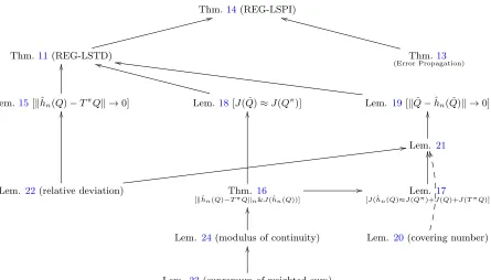
not fixed, but is a random function ˆQ. The same is true for the other optimization problem as well. The coupling of the optimization problems makes the analysis more complicated than the usual supervised learning type of analysis. The dependencies between all the results that lead to the proof of Theorem 14 is depicted in Figure2 in AppendixB.
In order to obtain fast convergence rates, we use concepts and techniques from the empirical process theory such as the peeling device, the chaining technique, and the modulus of continuity of the empirical process, cf. e.g., van de Geer (2000). By focusing on the behavior of the empirical process over local subsets of the function space, these techniques allow us to study the deviations of the process in a more refined way compared to a global approach that studies the supremum of the empirical process in the whole function space. These techniques are crucial to obtain a fast rate for large function spaces. We discuss them in more detail as we proceed in the proofs.
15. The Pinsker constant determines the effect of the noise variance too. We do not present such information in our bounds. Also note that most aforementioned results, except Golubev and Nussbaum (1990), consider a normal noise model, which is different from our bounded noise.
16. This is obtained by using Corollary 3 ofSteinwart et al.(2009) after substituting A2(λ) by its upper
bound λkfk2
H, which is valid whenever f ∗ ∈ H
We mentioned earlier that one can actually reuse a single data set in all iterations. To keep the presentation more clear, we keep the current setup. The reason behind this can be explained better after the proof of Theorem 11. But note that from the convergence-rate point of view, the difference between reusing data or not is insignificant. If we have a batch of data with size nand we divide it intoK chunks and only use one chunk per iteration of API, the rate would be O((Kn)−1+1α). For finite K, or slowly growingK, this is essentially
the same asO(n−1+1α).
5.2 Error Propagation in API
Consider an API algorithm that generates the sequence ˆQ(0) → π1 →Qˆ(1) → π2 → · · · → ˆ
Q(K−1) → π
K, where πk is the greedy policy w.r.t. Qˆ(k−1) and ˆQ(k) is the approximate
action-value function for policyπk. For the sequence ( ˆQ(k))Kk=0−1, denote the Bellman
Resid-ual (BR) of the kth action-value function by
εBRk = ˆQ(k)−TπkQˆ(k). (31) The goal of this section is to study the effect of theν-weightedL2-norm of the Bellman residual sequence (εBRk )kK=0−1 on the performance loss kQ∗−QπKk
1,ρ of the resulting policy
πK. Because of the dynamical nature of the MDP, the performance loss kQ∗−QπKkp,ρ
depends on the difference between the sampling distribution ν and the future state-action distribution in the form of ρPπ1Pπ2· · ·. The precise form of this dependence is formalized
in Theorem13, which is a slight modification of a result byFarahmand et al. (2010).17 Before stating the results, we define the following concentrability coefficients that are used in a change of measure argument, see e.g.,Munos(2007);Antos et al.(2008b); Farah-mand et al.(2010).
Definition 12 (Expected Concentrability of Future State-Action Distributions)
Given the distributions ρ, ν ∈ M(X × A), an integer m ≥0, and an arbitrary sequence of stationary policies(πm)m≥1, letρPπ1Pπ2· · ·Pπm ∈ M(X ×A)denote the future state-action
distribution obtained when the first state-action is distributed according to ρ and then we follow the sequence of policies (πk)mk=1. Define the following concentrability coefficients:
cPI1,ρ,ν(m1, m2;π),
E
d ρ(Pπ∗)m1(Pπ)m2
dν (X, A)
2
1 2
,
with (X, A) ∼ ν. If the future state-action distribution ρ(Pπ∗)m1(Pπ)m2 is not absolutely
continuous w.r.t. ν, then we take cPI1,ρ,ν(m1, m2;π) =∞.
In order to compactly present our results, we define the following notation:
ak =
(1−γ)γK−k−1
1−γK+1 . (0≤k < K) (32)
17. The difference of these two results is in the way the norm of functions from the spaceF|A|