A study on approximate solutions and accuracy of parallel algorithms for solving system of ODEs

(1)

_______________

*_{Corresponding author}

E-mail address: [email protected] Received January 23, 2019

110 J. Math. Comput. Sci. 10 (2020), No. 1, 110-135

https://doi.org/10.28919/jmcs/4006 ISSN: 1927-5307

A STUDY ON APPROXIMATE SOLUTIONS AND ACCURACY OF PARALLEL

ALGORITHMS FOR SOLVING SYSTEM OF ODES

A. HASAN*

_{Department of Mathematics, Faculty of Science, Jazan University, Jazan, KSA}

Copyright © 2020 the author(s). This is an open access article distributed under the Creative Commons Attribution License, which permits unrestricted use, distribution, and reproduction in any medium, provided the original work is properly cited.

Abstract. The purpose of this paper is, to study the numerical computation of system of ordinary differential equations of first order with initial value problems and all steps of parallel algorithms of R.K. methods are tested in MATLAB (2009a) [2]. In this part, we use four classical RK2 order methods to introduce the basic ideas associated with initial value problems for solving system of ODEs of two or more equations. At the end we make a comparison between these numerical methods for approximate solutions and numerical errors. Numerical examples are given to illustrate the computational accuracy and robustness of these parallel algorithms.

Keywords: system of ODEs; RK2 methods; Matlab; scientific computation; accuracy and efficiency; stability analysis.

2010 AMS Subject Classification: 34A45.

1. I

NTRODUCTION

Numerical Analysis is the area of mathematics and computer science that creates

algorithm and implements numerical methods for solving the problems of continuous

mathematics. In the field of Engineering and Science, we come across physical and natural

(2)

equations. Solving system of linear simultaneous differential equations is one of the most

important and challenging problems in science and engineering applications. It arises in a wide

variety of practical applications in Physics, Chemistry, Biosciences, Engineering, etc. System of

linear differential equations arises in various theoretical research fields as well as applications in

science and engineering. After the availability of computers, we go to numerical methods which

are suited for computer operations. For example, system of Lorentz equations and system of

coupled equations, deflection of a beam, etc. are represented by differential equations. Hence

solution of differential equation is a necessity in such studied. There are number of differential

equations which we studied in calculus to get closed form solutions. But all differential equations

do not possess closed form solutions or finite form solutions. Even they possess closed form

solutions; we do not know the method of getting it. In such situations depending upon the need

of the hour, we go in for numerical solutions of differential equations. In researches, especially

after the advent of computer, the numerical solutions of the differential equations have becomes

easy for manipulation. The dynamic behavior of systems is an important subject. A mechanical

system involves displacements,

velocities, and accelerations. An electric or electronic system

involves voltages, currents, and time derivatives of these quantities. An equation that involves

one or more derivatives of the unknown function is called an ordinary differential equation,

abbreviated as Ode. The problems of solving an ode are classified into initial-value problems and

boundary value problems, depending on how the conditions at the endpoints of the domain are

specified. All the conditions of an initial-value problem are specified at the initial point. On the

other hand, the problem becomes a boundary-value problem if the conditions are needed for both

initial and final points. The ode in the time domain are initial-value problems, so all the

conditions are specified at the initial time, such as x = 0. For notations, we use x as an

independent variable. It is important to note that our focus here is on the practical use of

numerical methods in order to solve some typical problems, not to present any consistent

theoretical background. Today there are numerous methods that produce numerical

approximations to the solution of differential equations. There are many excellent and exhaustive

texts on these subjects that may be consulted. [3-7]. Our purpose is here, to compare the

accuracy of various algorithms and how we can solve the systems of ODEs numerically and also

(3)

1.1. DEFINITION AND NOTATION.

The system of ordinary differential equations

considers has the form:

𝑑𝑦_𝑑𝑥

= 𝑓(𝑥, 𝑦(𝑥)), 𝑦(𝑥

0

) = 𝑦

0

, 𝑥 ∈ [𝑥

0

, 𝑥

𝑛

]

(i)

Here y(x) and f(x, y) are vector -valued functions

𝑦(𝑥) = (𝑦

₁

(𝑥) , 𝑦

2

(𝑥), 𝑦

3

(𝑥), … … … … . 𝑦

𝑚

(𝑥))

,

𝑓(𝑥, 𝑦) = (𝑓

₁

(𝑥, 𝑦) , 𝑓

₂

(𝑥, 𝑦), 𝑓

₃

(𝑥, 𝑦), … … … … . 𝑓

_𝑚

(𝑥, 𝑦))

,

so that we are dealing with m simultaneous first-order equations.

Definition:

The function

𝑓(𝑥, 𝑦

₁

, 𝑦

₂

… . 𝑦

_𝑚

)

, defined on the set D = {(x, y1,y2, . . . , ym) | a ≤ x ≤

b and − ∞ < yi < ∞, for each i = 1, 2,. . . , m} is said to satisfy a Lipschitz condition on D in the

variables y1, y2, . . . , ym if a constant L > 0 exists with

|𝑓(𝑥, 𝑦

1

, 𝑦

2

… . 𝑦

𝑚

) − 𝑓(𝑥, 𝑧

1

, 𝑧

2

… . 𝑧

𝑚

) | ≤ 𝐿 ∑

𝑗=𝑚𝑗=1

|𝑦

𝑗

− 𝑧

𝑗

|

(ii)

for all (x, y1, . . . , ym) and (x, z1, . . . , zm) in D. By using the Mean Value Theorem, it can be

shown that if f and its first partial derivatives are continuous on D and if

∂f (x, y1, y2. . . , ym) / ∂yi ≤ L, for each i = 1, 2, . . . , m

and all (x, y1, . . . , ym) in D, then f satisfies a Lipschitz condition on D with Lipschitz constant L

[3]. A basic existence and uniqueness theorem follows.

Theorem:

Suppose that D = {(x, y1, y2, . . ., ym) | a ≤ x ≤ b and − ∞ < yi < ∞, for each i = 1, 2,. . .

, m}, and let fi(x, y1, . . . , ym), for each i = 1, 2, . . . , m, be continuous and satisfy a Lipschitz

condition on D. The system of first-order differential equations (1), subject to the initial

conditions (1), has a unique solution y1(x), . . . , ym(x), for a ≤ x ≤ b.

Methods to solve systems of first-order differential equations are generalizations of the methods

for a single first-order equation presented.[3]

2. M

ATERIALS AND

M

ETHODS

Numerical methods are commonly used for solving mathematical problems that are

formulated in science and engineering where it is difficult or even impossible to obtain exact

solutions. Only a limited number of differential equations can be solved analytically. Numerical

methods, on the other hand, can give an approximate solution to (almost) any equation. Literal

implementation of this procedure results in Euler’s method, which is, however, not

(4)

Among one of them is Runge-Kutta methods. Now, we are interested to talk about Runge Kutta

methods. In the differential equation

𝑦

′

= 𝑓(𝑥, 𝑦)

on the interval [xj, xj+1] we get [1]

Second Order Explicit Runge Kutta Methods:

Consider the following Second Order Runge

kutta methods with two slopes

y

j+1

= y

j

+ [w

1

k

1

+ w

2

k

2

]

(2)

k1 = h f (xj , yj)

k2 = h f (xj+c2h, yj+a21k1)

where k1 and k2 are mention above. Thus we have four parameters c2, a21, w1 and w2 are chosen

to make

y

_j+1

closer to

y (x

_j+1

)

.and to be determined. The values of c2, a21, w1 and w2

are

evaluated by setting the second order equation to Taylor series expansion to the second order

term. Now Taylor series expansion about xj gives

𝑦(𝑥

_𝑗+1

) = 𝑦(𝑥

_𝑗

) + ℎ𝑦

′

(𝑥

_𝑗

) +

ℎ

2

2!

𝑦

′′

(𝑥

𝑗

) +

ℎ3

3!

𝑦

′′′

(𝑥

𝑗

) … … … …

𝑦(𝑥

_𝑗+1

) = 𝑦(𝑥

_𝑗

) + ℎ𝑓(𝑥

_𝑗

, 𝑦(𝑥

_𝑗

)) +

ℎ_2!2

(𝑓

_𝑥

+ 𝑓𝑓

_𝑦

) +

ℎ_3!3

[𝑓

_𝑥𝑥

+ 2𝑓𝑓

_𝑥𝑦

+ 𝑓

2

_𝑓

𝑦𝑦

+ 𝑓

𝑦

(𝑓

𝑥

+

𝑓𝑓

_𝑦

)] + ⋯ … … … ..

(3)

We also have k1 = h fj

k2 = h f (xj+c2h , yj+a21hfj)

k2 = h[fj+h(c2fx+a21ffy)xj+

ℎ

2

2!

(c

2

_𝑓

𝑥𝑥

+2c2a21

𝑓𝑓

𝑥𝑦

+

𝑎

212

𝑓

2

𝑓

𝑦𝑦

)+………..]

Putting the values of k1 and k2 in (2) we get

y

j+1

= y

j

+ (w

1

+ w

2

)h𝑓

𝑗

+ ℎ

2

(w

2

c

2

𝑓

𝑥

+ w

2

a

21

𝑓𝑓

𝑦

) +

ℎ

3

2

w

2

(𝑐

2 2

_𝑓

𝑥𝑥

+ 2𝑐

2

𝑎

21

𝑓𝑓

𝑥𝑦

+

𝑎

₂₁2

_𝑓

2

_𝑓

𝑦𝑦

) + ⋯ ….

(4)

Comparing the coefficients of h and h

2

_{in (3) and (4) we obtain}

w

₁

+ w

₂

= 1

w

2

c

2

=

1₂

w

₂

a

₂₁

=

1 2

Thus we get three equations of four unknowns and their solution is

,

a

₂₁

= c

₂

,

w

₂

=

_2c1

2

, 𝑎𝑛𝑑 w

1

= 1 −

1 2c2

(5)

y

_j+1

= y

_j

+ (1 −

_2c1

2

)k

1

+

1

2c2

k

2

(5)

Where k1 = h f (xj , yj)

k2 = h f (xj+c2h, yj+c2k1)

The free parameter c2 is usually taken between 0 and 1. Sometimes c2 is chosen such that one of

the wi’s in the formula (2) is zero. For example, the choice c2 =1/2 makes w1=0

Case (i) If c2=1/2, we get

k1 = h f (xj , yj)

k2 = h f (xj+h/2, yj+k1/2)

y

j+1

= y

j

+ k

2

(6)

which is called Mid-point method. It reduces to the mid-point quadrature rule when f(x,y) is

independent of y.

Case (ii). If c2=1, we get k1 = h f (xj , yj)

k2 = h f (xj+h , yj+k1)

y

_j+1

= y

_j

+

1₂

[k

₁

+ k

₂

]

(7)

Which is called Heun’s Method?

Case (iii). If c2=2/3 we get k1 = h f (xj , yj)

k2 = h f (xj+2/3 h , yj+2/3 k1)

y

_j+1

= y

_j

+

1₄

[k

₁

+ 3k

₂

]

(8)

Which is called nearly Optimal method. It may be noted that the explicit Runge Kutta methods

using two evaluations of f have one arbitrary parameter and have produced second order

methods.

Case (iv). If c2=3/4, we get k1 = h f (xj, yj)

k2 = h f (xj+3/4 h , yj+3/4 k1)

y

_j+1

= y

_j

+

1₃

[k

₁

+ 2k

₂

]

(9)

Which is called Raltson’s Method and have two functions of evaluations.

Ralston (1962) and

Ralston and Rabinowitiz (1978) determined that choosing ω2 = 2/3 provides a minimum bound

on the truncation error for the second order RK algorithms.[7]

(6)

𝑦(𝑥) = 𝑦(𝑥

₀

)𝑒

λ(𝑥−𝑥0)

= 𝑦

0

𝑒

λ(𝑥−𝑥0)

(11)

Substituting

𝑥 = 𝑥

𝑗+1

and

𝑥 = 𝑥

𝑗

in (11) and dividing, we get

𝑦(𝑥

_𝑗+1

) = 𝑦(𝑥

_𝑗

)𝑒

λ(𝑥𝑗+1−𝑥𝑗)

= 𝑦(𝑥

𝑗

)𝑒

λℎ

= 𝐸(

λ

ℎ)𝑦(𝑥

𝑗

)

(12)

Thus the numerical method is defined by above equation. Now applying the test equation in RK

method of order

y

_j+1

= y

_j

+ (1 −

_2c1

2

)k

1

+

1 2c2

k

2

Where

𝑘

₁

= ℎ𝑓(𝑥

_𝑗

, 𝑦

_𝑗

) =

λ

ℎ𝑦

_𝑗

𝑘

₂

= h f (𝑥

_𝑗

+ 𝑐

₂

h , 𝑦

_𝑗

+ 𝑐

₂

𝑘

₁

) =

λ

ℎ(𝑦

_𝑗

+ 𝑐

₂

𝑘

₁

) =

λ

ℎ[1 + 𝑐

₂

λ

ℎ]𝑦

_𝑗

y

_j+1

= y

_j

+ (1 −

_2c1

2

)

λ

ℎ𝑦

𝑗

+

1

2c2

λ

ℎ[1 + 𝑐

2

λ

ℎ]𝑦

𝑗

y

j+1

= [1 + (1 −

_2c1

2

)

λ

ℎ +

1

2c2

λ

ℎ(1 + 𝑐

2

λ

ℎ)]𝑦

𝑗

y

_j+1

= [1 +

λ

ℎ +

1₂

(λ

ℎ)

2

] 𝑦

_𝑗

= 𝐸(

λ

ℎ)𝑦

_𝑗

(13)

Hence the propagation factor

𝐸(

λ

ℎ)

is independent of the parameter c2 .Therefore the stability

intervals or regions of all second order Runge kutta methods is same. Now for

λ

real and

λ

< 0,

the condition

|𝐸(

λ

ℎ)| = |1 +

λ

ℎ +

1₂

(

λ

ℎ)

2

| < 1

|𝐸(

λ

ℎ)| = |1 +

z

+

1 2

𝑧

2

_{| < 1}

is satisfied when

λ

ℎ ∈ (−2,0)

Hence the region of stability of second order is

(−2, 0)

. The plots

of the stability regions for the second -order Runge-Kutta algorithms is shown in below Figure.

This stability region is larger than those of multi-step methods. In particular, the stability regions

of the stage schemes grow with increasing accuracy while the stability regions of

multi-step methods decrease with increasing accuracy. When analyzing multi-multi-step methods, the next

step would be to determine the locations in the λh-plane of the stability boundary (i.e. where |w|

= 1). This however is not easy for Runge-Kutta methods and would require the solution of a

higher-order polynomial for the roots. Instead, the most common approach is to simply rely on a

contour plotter in which the λh-plane is discretized into a finite set of points and |w| is evaluated

(7)

Then, the |w| = 1 contour can be plotted. Above Figure is Stability boundaries for second-order

Runge-Kutta algorithms (stable within the boundaries).

2.5. MATLAB CODES:

According to

[10-11].

Write all programs in M-file and save it as

midpoint.m, heun.m, Optimal.m, Raltson.m,

function [x,y]=systMidpoint(g,x0,xN,N,y0)

h=(xN-x0)/(N); x=[x0:h:xN]; y=zeros(length(y0),length(x)); y(:,1)=y0;

for n=1:1:N

k1=h*g(x(n),y(:,n));

k2=h*g(x(n)+h/2,y(:,n)+k1/2);

y(:,n+1)=y(:,n)+k2;

end

function [x,y]=systHeun(g,x0,xN,N,y0)

h=(xN-x0)/(N); x=[x0:h:xN]; y=zeros(length(y0),length(x)); y(:,1)=y0;

for n=1:1:N,

k1=h*g(x(n),y(:,n));

k2=h*g(x(n)+h,y(:,n)+k1);

y(:,n+1)=y(:,n)+1/2*(k1+k2);

Stability analysis of second order Runge kutta methods

Real(lamda*h)

Im

ag

(la

m

bd

a*

h)

-3 -2 -1 0 1 2 3

(8)

end,

end

function [x,y]=systOptimal(g,x0,xN,N,y0)

h=(xN-x0)/(N); x=[x0:h:xN]; y=zeros(length(y0),length(x)); y(:,1)=y0;

for n=1:1:N

k1=h*g(x(n),y(:,n));

k2=hg(x(n)+2/3h,y(:,n)+2/3*k1);

y(:,n+1)=y(:,n)+1/4(k1+3k2);

end

function [x,y]=systRaltson(g,x0,xN,N,y0)

h=(xN-x0)/(N); x=[x0:h:xN]; y=zeros(length(y0),length(x)); y(:,1)=y0;

for n=1:1:N

k1=h*g(x(n),y(:,n));

k2=hg(x(n)+3/4h,y(:,n)+3/4*k1);

y(:,n+1)=y(:,n)+1/3(k1+2k2);

end

Call functions for example 1

g = @(x,y)[-2y(1)+y(2)+2sin(x);y(1)-2y(2)+2(cos(x)-sin(x))]; [x,y1]=systHeun(g,0,2,10,[2

3]); [x,y2]=systMidpoint(g,0,2,10,[2 3]);

[x,y3]=systOptimal(g,0,2,10,[2 3]);

[x,y4]=systRaltson(g,0,2,10,[2 3]);

gexact = @(x,y)[2exp(-x)+sin(x);2exp(-x)+cos(x)];

xe=[0:0.2:2];

ye=gexact(xe);

(9)

g = @(x,y)[y(2);-2y(1)-2exp(x)+1;-y(1)-exp(x)+1]; [x,y1]=systHeun(g,0,2,10,[1 0 1]);

[x,y2]=systMidpoint(g,0,2,10,[1 0 1]);

[x,y3]=systOptimal(g,0,2,10,[1 0 1]);

[x,y4]=systRaltson(g,0,2,10,[1 0 1]);

gexact = @(x,y)[cos(x)+sin(x)-exp(x)+1;-sin(x)-exp(x)+cos(x);sin(x)+cos(x)];

xe=[0:0.2:2];

ye=gexact(xe);

3. C

ONVERGENCE

A

NALYSIS OF

M

ETHODS

The numerical solutions yi

will contain errors. We shall be concerned with the

effect of these errors on the solutions, To finding the numerical solution of ordinary differential

equations, two types of errors occurs. Round-off errors and Truncation errors. Rounding errors

originate from the fact that computer can only represent numbers using a fixed and limited

number of significant figures. Thus, such numbers cannot be represented exactly in computer

memory. The discrepancy introduced by this limitation is called Round-off error. Truncation

error in numerical analysis arises when approximations are used to estimate some quantity. The

accuracy of the solution will depend on how small we take the step size

ℎ

. A numerical method

is said to be convergent if the numerical solution approaches the exact solution as the step size

ℎ

goes to 0. A method is convergent if, as more grid points are taken or step size is decreased.[8]

4. N

UMERICAL

R

ESULTS AND

C

OMPARATIVE

D

ISCUSSION

In this section, we employ the different techniques, obtained in this paper to solve

system of simultaneous the ordinary differential equations with initial value problems and

compare them. We use the stopping criteria up to fifteen decimal places. We have

𝑇

_𝑖+1

=

𝑦(𝑡

_𝑖+1

) − 𝑦

𝑖+1

, 𝑖 = 0,1, … … … , 𝑁 − 1

for computer programs (2010) [9]. All programs are

written in Matlab 2009a. Let us consider the initial value

Problem1.

𝑑𝑦1

𝑑𝑥

= −2𝑦

1

+ 𝑦

2

+ 2 sin(𝑥), 𝑦

1

(0) = 2 ,

𝑥 ∈ [0, 2]

𝑑𝑦_𝑑𝑥2

= 𝑦

₁

− 2𝑦

₂

+ 2(cos(𝑥) − sin(𝑥)), 𝑦

₂

(2) = 3,

𝑥 ∈ [0, 2]

(10)

𝑦

₂

(𝑥) = 2𝑒

−𝑥

+ (cos(𝑥))

Problem2.

𝑑𝑦_𝑑𝑥1

= 𝑦

₂

, 𝑦

₁

(0) = 1

,

𝑥 ∈ [0, 2]

𝑑𝑦2

𝑑𝑥

= −𝑦

1

− 2𝑒

𝑥

_{+ 1, 𝑦}

2

(0) = 0,

𝑥 ∈ [0, 2]

𝑑𝑦_𝑑𝑥3

= −𝑦

₁

− 𝑒

𝑥

+ 1, 𝑦

₃

(0) = 1

,

𝑥 ∈ [0, 2]

The exact solution for this problem is

𝑦

1

(𝑥) = cos(𝑥) + sin(𝑥) − 𝑒

𝑥

+ 1

𝑦

₂

(𝑥) = −sin (𝑥) − 𝑒

𝑥

+ cos(𝑥)

𝑦

₃

(𝑥) = − sin(𝑥) + cos(𝑥)

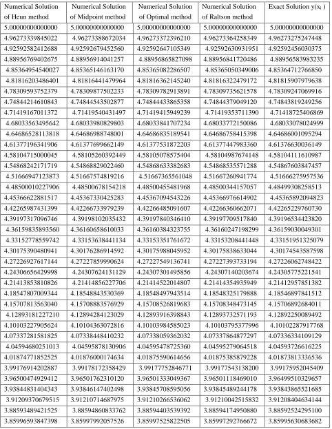
Table1. Numerical and Exact solutions of various techniques at grid points when h=0.2

Numerical Solution of Heun method

Numerical Solution of Midpoint method

Numerical Solution of Optimal method

Numerical Solution of Raltson method

Exact Solution y(xi )

(11)

Table2. Numerical and Exact solutions of various techniques at grid points when h=0.1

(12)

Table3. Numerical and Exact solutions of various techniques at grid points when h=0.05

(13)

Table4.Numerical and Exact solutions of various techniques at grid points when h=0.025

(14)

(15)

Table 5. Numerical and Exact solutions of various methods at grid points when h=0.0125

(16)

(17)

(18)

1.96075079681901 1.96076740678281 1.96076185966146 1.96075909002356 1.96075282886548 1.93799604925743 1.93801248438912 1.93800699544956 1.93800425493843 1.93799813421655 1.91521394635428 1.91523020273251 1.91522477328288 1.91522206255220 1.91521607929299 1.89240462612902 1.89242069987718 1.89241533121074 1.89241265090674 1.89240680207464 1.86956827335695 1.86958416064359 1.86957885403855 1.86957620479994 1.86957048729942 1.84670511901234 1.84672081605151 1.84671557277095 1.84671295522886 1.84670736590650 1.82381543971091 1.82383094276260 1.82382576405430 1.82382317883220 1.82381771447873 1.80089955715169 1.80091486252220 1.80090974961853 1.80090719733219 1.80090185468448 1.77795783755826 1.77797294160053 1.77796789571833 1.77796537697573 1.77796015271884 1.75499069111922 1.75500559023329 1.75500061257373 1.75499812797500 1.75499301874409 1.73199857142821 1.73201326206151 1.73200835380997 1.73200590394737 1.73200090632967 1.70898197492314 1.70899645357091 1.70899161589685 1.70898920135466 1.70898431189140 1.68594144032493 1.68595570353054 1.68595093758743 1.68594855894191 1.68594377413020 1.66287754807562 1.66289159243094 1.66288689935607 1.66288455717539 1.66287987347013 1.63979091977582 1.63980474192159 1.63980012283599 1.63979781768019 1.63979323149588 1.61668221762175 1.61669581424786 1.61669127025619 1.61668900267713 1.61668451038974 1.59355214384153 1.59356551168742 1.59356104387786 1.59355881441911 1.59355441236788 1.57040144013108 1.57041457598606 1.57041018543017 1.57040799462703 1.57040367911625 1.54723088708947 1.54724378779301 1.54723947554565 1.54723732392504 1.54723309122584 1.52404130365369 1.52405396609578 1.52404973319499 1.52404762127542 1.52404346762749 1.50083354653302 1.50084596765448 1.50084181512138 1.50083974341288 1.50083566502623 1.47760850964291 1.47762068643566 1.47761661527434 1.47761458427844 1.47761057733507 1.45436712353837 1.45437905304580 1.45437506424323 1.45437307445287 1.45436913510847 1.43111035484705 1.43112203416426 1.43111812869017 1.43111618058968 1.43111230497531 1.40783920570177 1.40785063197588 1.40784681078270 1.40784490484774 1.40784108907145 1.38455471317281 1.38456588360326 1.38456214762598 1.38456028432350 1.38455652447196 1.36125794869976 1.36126886053857 1.36126521069467 1.36126339048285 1.36125968262298 1.33795001752311 1.33796066807516 1.33795710526451 1.33795532859274 1.33795166877323 1.31463205811546 1.31464244473875 1.31463896984355 1.31463723715234 1.31463362140530 1.29130524161255 1.29131536171847 1.29131197560312 1.29131028732409 1.29130671166654 1.26797077124397 1.26798062229754 1.26797732580859 1.26797568236444 1.26797214279983 1.24462988176369 1.24463946128383 1.24463625524986 1.24463465705430 1.24463114957407 1.22128383888039 1.22129314444014 1.22129002967172 1.22128847712944 1.22128499771445 1.19793393868766 1.19794296791443 1.19793994520402 1.19793843871065 1.19793498333268 1.17458150709404 1.17459025766981 1.17458732779168 1.17458586773376 1.17458243235696 1.15122789925296 1.15123636891452 1.15123353262470 1.15123211937964 1.15122869996196 1.12787449899266 1.12788268553184 1.12787994356802 1.12787857750404 1.12787516999864 1.10452271824606 1.10453061950990 1.10452797259138 1.10452665406752 1.10452325442416 1.08117399648062 1.08118161037159 1.08117905919920 1.08117778856526 1.08117439273169 1.05782980012825 1.05783712460445 1.05783466986050 1.05783344745699 1.05783005138031 1.03449162201530 1.03449865509064 1.03449629743884 1.03449512359699 1.03449172322499

(19)

Table.6. Estimation of average % errors by various methods at different step size h

Step size h Average % Error in Midpoint method

Average % Error in Heun method

Average %Error in Optimalmethod

Average %Error in Raltson method h=0.2 p2=9.804732502 677809e-001 p1=1.490367120 678143e+000 p3=1.1060551209701 10e+000 p4=1.1871343958564 42e+000 h=0.1 p2=3.47504795215030 8e-001 p1=5.2851196716503 65e-001 p3=3.9833419508330 45e-001 p4=4.2723398234604 53e-001 h=0.05 p2=7.54606238799641 5e-002 p1=1.0985600082081 12e-001 p3=8.4892578515347 21e-002 p4=9.0347788915291 19e-002 h=0.025 p2=2.41242827674237 2e-002 p1=3.5632497169804 07e-002 p3=2.7478122509415 96e-002 p4=2.9327572298309 16e-002 h=0.0125 p2=5.80408547079670 7e-003 p1=8.4994213086670 43e-003 p3=6.5872554942438 05e-003 p4=7.0196919845357 70e-003

0 0.2 0.4 0.6 0.8 1 1.2 1.4 1.6 1.8 2

0 1 2 3 4 5 6 7

number of subintervals

m ax im um % e rr or s

Fig1-Comparison of % errors when h=0.2

(20)

0 0.2 0.4 0.6 0.8 1 1.2 1.4 1.6 1.8 2

0 1 2 3 4 5 6 7

m

a

x

im

u

m

%

e

rr

o

rs

Huen method Midpoint method Optimal method Raltson method

0 0.2 0.4 0.6 0.8 1 1.2 1.4 1.6 1.8 2

0 0.5 1 1.5

m

a

x

im

u

m

%

e

rr

o

rs

(21)

0 0.2 0.4 0.6 0.8 1 1.2 1.4 1.6 1.8 2

0 0.2 0.4 0.6 0.8 1 1.2 1.4

number of subintervals 80

m

a

x

im

u

m

%

e

rr

o

rs

0 0.2 0.4 0.6 0.8 1 1.2 1.4 1.6 1.8 2

0 0.05 0.1 0.15 0.2 0.25 0.3 0.35

m

a

x

im

u

m

%

e

rr

o

rs

(22)

Problem 2.

Table 7. Estimation of % errors by various methods at end point with step size h

Step size h

Average % Error

in Midpoint

method

Average %

Error in

Heun method

Average %

Error in

Optimal method

Average %

Error in Raltson

method

h=0.2

p2 =4.540740607

540969e+000

p1=6.5619859201

00095e+000

p3=5.1109776404

57402e+000

p4= 5.467626711

817050e+000

h=0.1

p2 =

1.1477958972148

05e+000

p1 =

1.6473117634616

57e+000

p3=

1.3011682115037

21e+000

p4=

1.3869795105165

71e+000

h=0.05

p2=

2.8835044462315

04e-001

p1 =

4.1231117313856

71e-001

p3=

3.2807771188342

93e-001

p4=

3.4904812222840

70e-001

h=0.025

p2=

7.2248003205440

49e-002

p1 =

1.0310829509984

61e-001

p3=

8.2354213720311

96e-002

p4=

8.7531911557116

36e-002

h=0.0125

p2=

1.8080995090460

13e-002

p1 =

2.5778784328693

92e-002

p3=

2.0629405539850

26e-002

p4=

2.1915408439673

85e-002

0 0.2 0.4 0.6 0.8 1 1.2 1.4 1.6 1.8 2

0 20 40 60 80 100 120

m a x im u m % e rr o rs

(23)

0 0.2 0.4 0.6 0.8 1 1.2 1.4 1.6 1.8 2

0 5 10 15 20 25 30

m

a

x

im

u

m

%

e

rr

o

rs

0 0.2 0.4 0.6 0.8 1 1.2 1.4 1.6 1.8 2

0 1 2 3 4 5 6 7

m

a

x

im

u

m

%

e

rr

o

rs

(24)

0 0.2 0.4 0.6 0.8 1 1.2 1.4 1.6 1.8 2

0 0.5 1 1.5 2 2.5

m

a

x

im

u

m

%

e

rr

o

rs

0 0.2 0.4 0.6 0.8 1 1.2 1.4 1.6 1.8 2

0 0.5 1 1.5 2 2.5 3

m

a

x

im

u

m

%

e

rr

o

rs

(25)

Table8. Ratios of percentage error between different values of h

Step

Size h

Ratios % Error in

midpoint Method

Ratios % Error in

Huen Method

Ratios % Error in

Optimal Method

Ratios % Error in

Raltson Method

Problm1 Problm2 Prob1

Prob2

Prob1

Prob2

Prob1

Prob2

0.2

0.1

0.05

0.025 0.0125

2.8215

4.6051

3.1280

4.1564

= 2

2

3.9561

3.9806

3.9911

3.9958

= 2

2

2.8199

4.8110

3.0830

4.1923

=

2

3.9835

3.9953

3.9988

3.9997

= 2

2

2.7767

4.6922

3.0895

4.1714

= 2

2

3.9280

3.9660

3.9837

3.9921

= 2

2

2.7787

4.7288

3.0806

4.1779

= 2

2

3.9421

3.9736

3.9877

3.9941

= 2

2

From the Table6 and Table7.The calculated results are displayed for average percentage errors at

different step size. Reasonably good results are obtained even for a large step size and the

approximation can be improved by decreasing the step size. According to the results Midpoint

method give good result when compare with exact solution. Since midpoint method has

minimum error as compared to other methods. From the Table8 we see that when we reduce the

step size h/2 the ratios of % errors are equivalent to

2

. This verifies that each method is second

order RK method. Thus the accuracy of Midpoint method is good among them. Hence we

conclude that Midpoint method is most effective scheme overall.

5. C

ONCLUSIONS

The RK2 methods are simple methods of solving first-order system of ODE, particularly

suitable for quick programming because of their great simplicity, although their accuracy is not

high. First, the midpoint method is more accurate than other RK2 methods. Second, it is more

stable. The above plots shows the results obtained from different algorithms at different step size.

One can easily adopt this paper as needed for a different type of problems for solving system

ordinary differential equations for more variables first order linear equations. Inner working of

the numerical methods will be clear, especially for the students. In using numerical procedure,

such as Midpoint method, one must always keep in mind the question of whether the results are

accurate enough to be useful. In the preceding examples, the accuracy of the numerical results

(26)

the numerical computations we see that accuracy and efficiency of midpoint method is most

effective.

C

ONFLICT OF

I

NTERESTS

The author(s) declare that there is no conflict of interests.

R

EFERENCES

[1] M.K. Jain, S.R.K. Iyenger and R.K. Jain. Numerical methods for scientific and engineering computation. New Age International Publishers, 2010.

[2] The Math Works Inc. MATLAB: 7.8. The Math Works Inc., 2009a.

[3] R.L. Burden and J.D. Faris Numerical Analysis 9th _{Edition, Cenage Learning/Nels Education, Ltd. (2010)}

[4] A. Hasan, Numerical computation of initial value problem by various techniques, J. Sci. Arts 18 (2018), 19-32. [5] D. Eberly, stability analysis for systems of differential equations, Geometric Tools, (2008).

[6] C. B. Moler. Numerical Computing with MATLAB. Siam, 2011.

[7] J.R. Dormand and P.J. Prince. A family of embedded Runge-Kutta formulae. J. Comput. Appl. Math, 6(1980), 19-26,

[8] L. F. Shampine. Numerical Solution of Ordinary Equations. Chapman and Hall, 1997.

[9] C. F. Gerald and P.O. Wheatley, Applied Numerical Analysis. Pearson Education, India. (2004). [10]W. Shen. Lecture notes on Introduction to Numerical Computation 2012.